Optimization Problems with Stochastic Order …...Optimization Problems with Stochastic Order...

Optimization Problems with Stochastic OrderConstraints

Darinka Dentcheva

Stevens Institute of Technology, Hoboken, New Jersey, USA

Research supported by NSF awards CMII-0965702

Ann Arbor, February 28th 2013

Motivation

Risk-Averse Optimization Models

Choose a decision z ∈ Z , which results in a random outcomeG(z) ∈ Lp(Ω,F ,P) with “good" characteristics paying specialattention to low-probability-high-impact events.

Utility models apply a nonlinear transformation to the realizationsof G(z) (expected utility) or to the probability of events (rankdependent utility/distortion). Expected utility models optimizeE[u(G(z))]

Probabilistic / chance constraints impose prescribed probabilityon some events: P[G(z) ≥ η]

Mean–risk models optimize a composite objective of theexpected performance and a scalar measure of undesirablerealizationsE[G(z)]− %[G(z)] (risk/ deviation measures)Stochastic ordering constraints compare random outcomes usingstochastic orders and random benchmarks

Darinka Dentcheva Optimization and Stochastic Orders

Outline

1 Stochastic orders

2 Stochastic orders as constraints

3 Optimality conditions and dualityRelation to von Neumann utility theoryRelation to rank dependent utilityRelation to coherent measures of risk

4 Multivariate and Dynamic Orders

5 Numerical methods

6 ApplicationsPortfolio optimizationBeyond portfolio optimization


Integral Univariate Stochastic Orders

For X ,Y ∈ L1(Ω,F ,P)

X F

Y ⇔∫Ω

u(X (ω)) P(dω) ≥∫Ω

u(Y (ω)) P(dω) ∀ u(·) ∈ F

Collection of functions F is the generator of the order.

Generators

F1 =

nondecreasing functions u : R→ R

generates the usualstochastic order or first order stochastic dominance (X

(1) Y )Mann and Whitney (1947), Blackwell (1953), Lehmann (1955)

F2 =

nondecreasing concave u : R→ R

generates the secondorder stochastic dominance relation (X

(2) Y )Quirk and Saposnik (1962), Fishburn (1964), Hadar and Russell (1969)

F2 =

nondecreasing convex u : R→ R

generates theincreasing convex order (X ic Y ) counterpart of stochasticdominance of second order when small values are preferred


Stochastic Orders and Distribution Functions

For any X ∈ Lk (Ω,F ,P)(Ω,F ,P), we define

Distribution Functions

F1(X ; η) =

∫ η

−∞PX (dt) = PX ≤ η for all η ∈ R

Fk (X ; η) =

∫ η

−∞Fk−1(X ; t) dt for all η ∈ R, k = 2,3, . . .

The function F (k)X is nondecreasing for k ≥ 1 and convex for k ≥ 2.

Quantile function

F(−1)(X ; p) = infη : F1(X ; η) ≥ p, p ∈ (0,1)

Survival function

F 1(X ; η) = 1− F1(X ; η) = PX > η, η ∈ R


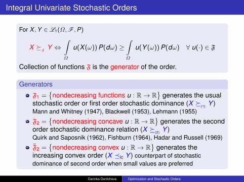
First Order Stochastic Dominance

-

-

0

1 6

ηµXµY

F1(X ; η)F1(Y ; η)

The usual stochastic order

X (1) Y ⇔ F1(X ; η) ≤ F1(Y ; η) for all η ∈ R

⇔ F(−1)(X ; p) ≥ F(−1)(Y ; p) for all 0 < p < 1.

⇔ F 1(X ; η) ≥ F 1(Y ; η) for all η ∈ R.


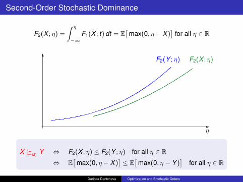
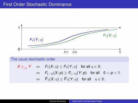
Second-Order Stochastic Dominance

F2(X ; η) =

∫ η

−∞F1(X ; t) dt = E

[max(0, η − X )

]for all η ∈ R

-

6

η

F2(Y ; η) F2(X ; η)

X (2) Y ⇔ F2(X ; η) ≤ F2(Y ; η) for all η ∈ R

⇔ E[

max(0, η − X )]≤ E

[max(0, η − Y )

]for all η ∈ R


Higher order relation

For any X ∈ Lk (Ω,F ,P)(Ω,F ,P), ‖X‖k =(E(|X |k )

) 1k and

F(k+1)(X , η) =1k !

∫ η

−∞(η− t)k PX (dt) =

1k !‖max

(0, η−X

)‖k

k ∀η ∈ R,

k th degree Stochastic Dominance (kSD), k ≥ 2

X (k) Y ⇔ Fk (X , η) ≤ Fk (Y , η) for all η ∈ R,

‖max(0, η − X

)‖k−1

k−1 ≤ ‖max(0, η − Y

)‖k−1

k−1

The generator

Fk contains all functions u : R→ R such that a non-increasing,left-continuous, bounded function ϕ : R → R+ exists such thatu(k−1)(η) = (−1)kϕ(η) for a.a. η ∈ R.


Second Order Dominance and Inverse Distribution Functions

Absolute Lorenz function (Max Otto Lorenz, 1905)

F(−2)(X ; p) =

∫ p

0F(−1)(X ; t) dt for 0 < p ≤ 1,

F(−2)(X ; 0) = 0 and F(−2)(X ; p) = +∞ for p 6∈ [0, 1].

Fenchel conjugate function of F : F ∗(p) = supupu − F (u)

Lorenz function and Expected shortfall are Fenchel conjugates

F(−2)(X ; ·) = [F2(X ; ·)]∗ and F2(X ; ·) = [F(−2)(X ; ·)]∗

Ogryczak - Ruszczynski (2002)

Second order dominance ≡ Relation between Lorenz function

X (2) Y ⇔ F(−2)(X ; p) ≥ F(−2)(Y ; p) for all 0 ≤ p ≤ 1.


Characterization of Stochastic Dominance by Lorenz Functions

6

-

1

F(−2)(X ; p)

F(−2)(Y ; p)

µx

µy

p

p p p p p p p p p p p p p p p p p p p p p p p p p p p p p p p p p p p p p p pp p p p p p p p p p p p p p p p p p p p p p p p p p p p p p p p p p p p p p p

0

X (2) Y ⇔ F(−2)(X ; p) ≥ F(−2)(Y ; p) for all 0 ≤ p ≤ 1.


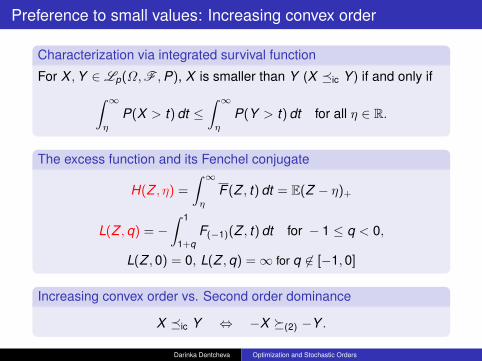
Preference to small values: Increasing convex order

Characterization via integrated survival function

For X ,Y ∈ Lp(Ω,F ,P), X is smaller than Y (X ic Y ) if and only if∫ ∞η

P(X > t) dt ≤∫ ∞η

P(Y > t) dt for all η ∈ R.

The excess function and its Fenchel conjugate

H(Z , η) =

∫ ∞η

F (Z , t) dt = E(Z − η)+

L(Z ,q) = −∫ 1

1+qF(−1)(Z , t) dt for − 1 ≤ q < 0,

L(Z ,0) = 0, L(Z ,q) =∞ for q 6∈ [−1,0]

Increasing convex order vs. Second order dominance

X ic Y ⇔ −X (2) −Y .


Characterization via Rank Dependent Utility Functions

W1 contains all continuous nondecreasing functions w : [0,1]→ R.W2 ⊂ W1 contains all concave subdifferentiable at 0 functions.

Theorem [DD, A. Ruszczynski, 2006]

(i) For all random variables X ,Y ∈ L1(Ω,F ,P) the relationX (1) Y holds if and only if for all w ∈ W1

1∫0

F(−1)(X ; p) dw(p) ≥1∫

0

F(−1)(Y ; p) dw(p) (1)

(ii) X (2) Y holds if and only if (1) is satisfied for all w ∈ W2.

Corollary

X ic Y holds if and only if (1) is satisfied for all convex functions wwhich are subdifferentiable at zero.

Quiggin (1982), Schmeidler (1986–89), Yaari (1987)


Acceptance Sets

For all k ≥ 1, Y - benchmark outcome in Lk−1(Ω,F ,P), [a,b] ⊆ R.

Acceptance sets Ak (Y ; [a,b]) = X ∈ Lk−1 : X (k) Y in [a,b]

Theorem

The set Ak (Y ; [a,b]) is convex and closed for all [a,b], all Y , andk ≥ 2 . Its recession cone has the form

A∞k (Y ; [a,b]) =

H ∈ Lk−1(Ω,F ,P) : H ≥ 0 a.s. on [a,b]

A1(Y ; [a,b]) is closed and Ak (Y ; [a,b]) ⊆ Ak+1(Y ; [a,b]) ∀k ≥ 1.Ak (Y ; [a, b]) is a cone pointed at Y if and only if Y is a constant in [a, b].

Theorem

If (Ω,F ,P) is atomless, then A2(Y ;R) = co A1(Y ;R) If Ω = 1..N,and P[k ] = 1/N, then A2(Y ;R) = co A1(Y ;R)

The result is not true for general probability spaces


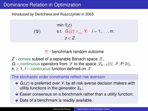
Dominance Relation in Optimization

Introduced by Dentcheva and Ruszczynski in 2003

min f (z)

(P) s.t. Gi (z) (ki )

Yi i = 1, . . . ,m,

z ∈ Z .

Yi - benchmark random outcome

Z - convex subset of a separable Banach space Z ,Gi – continuous operators from Z to the space Lki−1(Ω,F ,P;R),ki ≥ 1, f – continuous function defined on Z .

The stochastic order constraints reflect risk aversion

Gi (z) is preferred over Yi by all risk-averse decision makers withutility functions in the generator Fki ;Easier consensus on a benchmark rather than a utility function;Data of a benchmark is readily available.


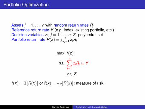
Portfolio Optimization

Assets j = 1, . . . ,n with random return rates RjReference return rate Y (e.g. index, existing portfolio, etc.)Decision variables zj , j = 1, . . . ,n, Z -polyhedral setPortfolio return rate R(z) =

∑nj=1 zjRj

max f (z)

s.t.n∑

j=1

zjRj Y

z ∈ Z

f (x) = E[R(x)

]or f (x) = −%

[R(x)

]: measure of risk.


All Statements are Equivalent

n∑j=1

zjRj (2) Y

F(−2)( n∑

j=1

zjRj ; p)≥ F(−2)(Y ; p) for all p ∈ [0,1]

continuum of CVaR constraints for every risk level p ∈ [0,1]

Eu(n∑

j=1

zjRj ) ≥ Eu(Y )

for all concave nondecreasing functions u (von Neuman-Morgenstern utility)1∫

0

F(−1)(n∑

j=1

zjRj ; p) dw(p) ≥1∫

0

F(−1)(Y ; p) dw(p)

for all concave nondecreasing functions w (rank dependent utility)


Second Order Dominance Constraints

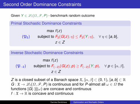
Given Y ∈ L1(Ω,F ,P) - benchmark random outcome

Primal Stochastic Dominance Constraints

max f (z)

(P2) subject to F2(G(z); η) ≤ F2(Y ; η), ∀ η ∈ [a,b],

z ∈ Z

Inverse Stochastic Dominance Constraints

max f (z)

(P−2) subject to F(−2)(G(z); p) ≥ F(−2)(Y ; p), ∀ p ∈ [α, β],

z ∈ Z

Z is a closed subset of a Banach space X, [α, β] ⊂ (0,1), [a,b] ⊂ RG : X→ L1(Ω,F ,P) is continuous and for P-almost all ω ∈ Ω thefunctions [G(·)](ω) are concave and continuousf : X→ R is concave and continuous


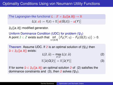
Optimality Conditions Using von Neumann Utility Functions

The Lagrangian-like functional L : Z × F2([a,b])→ RL(z,u) := f (z) + E

[u(G(z))− u(Y )

]F2([a,b]) modified generator.

Uniform Dominance Condition (UDC) for problem (P2)A point z ∈ Z exists such that inf

η∈[a,b]

F2(Y ; η)− F2(G(z); η)

> 0.

Theorem Assume UDC. If z is an optimal solution of (P2) thenu ∈ F2([a,b]) exists:

L(z, u) = maxz∈Z

L(z, u) (2)

E[u(G(z)

]= E

[u(Y )

](3)

If for some u ∈ F2([a,b]) an optimal solution z of (2) satisfies thedominance constraints and (3), then z solves (P2).


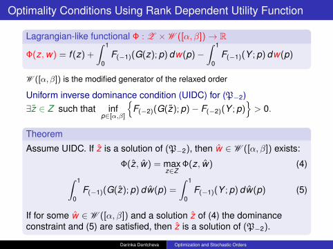
Optimality Conditions Using Rank Dependent Utility Function

Lagrangian-like functional Φ : Z ×W ([α, β])→ R

Φ(z,w) = f (z) +

∫ 1

0F(−1)(G(z); p) dw(p)−

∫ 1

0F(−1)(Y ; p) dw(p)

W ([α, β]) is the modified generator of the relaxed order

Uniform inverse dominance condition (UIDC) for (P−2)∃z ∈ Z such that inf

p∈[α,β]

F(−2)(G(z); p)− F(−2)(Y ; p)

> 0.

Theorem

Assume UIDC. If z is a solution of (P−2), then w ∈ W ([α, β]) exists:

Φ(z, w) = maxz∈Z

Φ(z, w) (4)∫ 1

0F(−1)(G(z); p) dw(p) =

∫ 1

0F(−1)(Y ; p) dw(p) (5)

If for some w ∈ W ([α, β]) and a solution z of (4) the dominanceconstraint and (5) are satisfied, then z is a solution of (P−2).


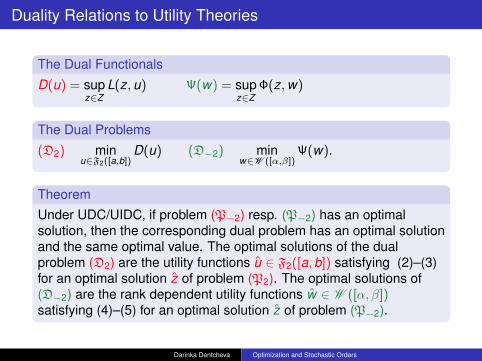
Duality Relations to Utility Theories

The Dual Functionals

D(u) = supz∈Z

L(z,u) Ψ(w) = supz∈Z

Φ(z,w)

The Dual Problems

(D2) minu∈F2([a,b])

D(u) (D−2) minw∈W ([α,β])

Ψ(w).

TheoremUnder UDC/UIDC, if problem (P−2) resp. (P−2) has an optimalsolution, then the corresponding dual problem has an optimal solutionand the same optimal value. The optimal solutions of the dualproblem (D2) are the utility functions u ∈ F2([a,b]) satisfying (2)–(3)for an optimal solution z of problem (P2). The optimal solutions of(D−2) are the rank dependent utility functions w ∈ W ([α, β])satisfying (4)–(5) for an optimal solution z of problem (P−2).


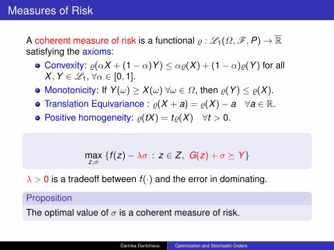
Measures of Risk

A coherent measure of risk is a functional % : L1(Ω,F ,P)→ Rsatisfying the axioms:

Convexity: %(αX + (1− α)Y ) ≤ α%(X ) + (1− α)%(Y ) for allX ,Y ∈ L1, ∀α ∈ [0,1].Monotonicity: If Y (ω) ≥ X (ω) ∀ω ∈ Ω, then %(Y ) ≤ %(X ).Translation Equivariance : %(X + a) = %(X )− a ∀a ∈ R.Positive homogeneity: %(tX ) = t%(X ) ∀t > 0.

maxz,σf (z)− λσ : z ∈ Z , G(z) + σ Y

λ > 0 is a tradeoff between f (·) and the error in dominating.

Proposition

The optimal value of σ is a coherent measure of risk.


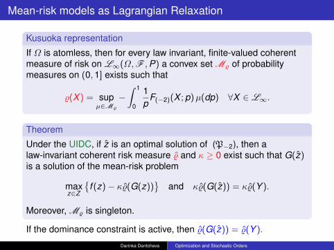
Mean-risk models as Lagrangian Relaxation

Kusuoka representation

If Ω is atomless, then for every law invariant, finite-valued coherentmeasure of risk on L∞(Ω,F ,P) a convex set M% of probabilitymeasures on (0,1] exists such that

%(X ) = supµ∈M%

−∫ 1

0

1p

F(−2)(X ; p)µ(dp) ∀X ∈ L∞.

Theorem

Under the UIDC, if z is an optimal solution of (P−2), then alaw-invariant coherent risk measure % and κ ≥ 0 exist such that G(z)is a solution of the mean-risk problem

maxz∈Z

f (z)− κ%(G(z))

and κ%(G(z)) = κ%(Y ).

Moreover, M% is singleton.

If the dominance constraint is active, then %(G(z)) = %(Y ).


The Implied Dominance Constraint

Given the problem

(R) maxX∈C

f (X )− κ%(X )

%(·) a coherent law invariant measure of risk and κ > 0rca([0,1]) - space of regular countably additive measures on [0,1].

Theorem If M% is compact∗ in rca([0,1]) and X is a solution ofproblem (R), then ∃ µ ∈M such that

%(X ) = −∫ 1

0

1p

F(−2)(X ; p) µ(dt),

and for every Y ∈ L1(Ω,F ,P) satisfying the conditions

F(−2)(Y ; t) ≤ F(−2)(X ; t), for all t ∈ [0,1],

F(−2)(Y ; t) = F(−2)(X ; t), for all t ∈ supp(µ),

the point X is also a solution of problem (P−2) with [α, β] = [0,1].


Portfolio Optimization Under Stochastic Dominance Constraints

Assets j = 1, . . . ,n, n = 719 with random returns RjDecision variables zj , j = 1, . . . ,n, Z -simplexPortfolio return G(z) =

∑Nj=1 zjRj

Reference return Y is the Standard and Poor 500 index.

max E[ n∑

j=1

zjRj]

subject ton∑

j=1

zjRj (2) Y

z ∈ Z

We use 248 realizations of the joint returns

The optimal portfolio

7 stocks with weights 10.98%, 7.08%, 21.79%, 13.19%, 36.51%,4.41% 6.04%, correspondingly; the expected return is 0.64% vs.-0.0359% of S&P 500


Implied Expected Utility

-5%

-4%

-3%

-2%

-1%

0%

-0.05 0.05 0.15 0.25Utility

return


Implied Rank Dependent Utility Function

-1.4

-1.2

-1

-0.8

-0.6

-0.4

-0.2

0

0.2

-0.1 6E-16 0.1 0.2 0.3 0.4 0.5 0.6

probability

dis

tort

ion


Implied Measure of Risk

0

0.05

0.1

0.15

0.2

0.25

0.3

0.35

0.1772 0.3102 0.3636 0.4093 0.4594 0.4967 0.5081 0.5570 0.5647 0.5750

probability level

wei

gh

t

%(X) = 0.1069AVaR0.1772(X) + 0.014AVaR0.3101(X) + 0.0274AVaR0.3636(X)

+ 0.0577AVaR0.4093(X) + 0.3073AVaR0.4594(X) + 0.2935AVaR0.4967(X)

+ 0.1077AVaR0.5081(X) + 0.0576AVaR0.557(X) + 0.0213AVaR0.5647(X)

+ 0.0066AVaR0.575(X)


Multivariate and Dynamic Orders

Consider X = (X1, . . . ,Xm) and Y = (Y1, . . . ,Ym) in L m1 (Ω,F ,P).

Coordinate Order

X sep(2) Y ⇔ Xt (2) Yt , t = 1, . . . ,m

Generator Fs all functions u(X ) =∑m

t=1 ui (Xi ) with concavenondecreasing ui : R→ R. Our earlier analysis covers this case.

Ignores temporal structure and dependency

Increasing Convex Order

X (icx) Y ⇔ E[u(X )

]≥ E

[u(Y )

]∀ u ∈ F

Generator Fa - all concave nondecreasing functions u : Rm → RHard to treat analytically, the generator is too rich

Proposed approach

Define the mutlivariate order via a family of univariate orders


Multivariate and Dynamic Orders: Definition

DefinitionA random vector X ∈ L m

1 dominates a random vector Y ∈ L m1 with

respect to the linear second-order dominance

(X lin(2) Y ) if c>X lin

(2) c>Y for all c ∈ S,

where S = c ∈ Rm+ : ‖c‖1 = 1.

If the set S contains non-increasing sequences, then lin(2) can be

used to compare sequences.

The linear order lin(2) implies the coordinate order Xi (2) Yi ,

i = 1, . . . ,m but is not equivalent to it.

Other definitions: A. Müller, D. Stoyan, Homem-de-Mello and Mehrotra: S is apolyhedron, or a compact convex set.


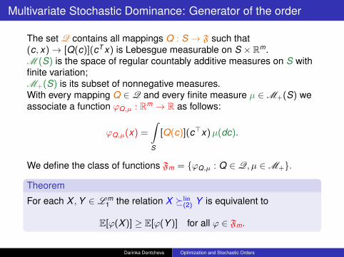
Multivariate Stochastic Dominance: Generator of the order

The set Q contains all mappings Q : S → F such that(c, x)→ [Q(c)](cT x) is Lebesgue measurable on S × Rm.M (S) is the space of regular countably additive measures on S withfinite variation;M+(S) is its subset of nonnegative measures.With every mapping Q ∈ Q and every finite measure µ ∈M+(S) weassociate a function ϕQ,µ : Rm → R as follows:

ϕQ,µ(x) =

∫S

[Q(c)](c>x)µ(dc).

We define the class of functions Fm = ϕQ,µ : Q ∈ Q, µ ∈M+.

Theorem

For each X ,Y ∈ L m1 the relation X lin

(2) Y is equivalent to

E[ϕ(X )] ≥ E[ϕ(Y )] for all ϕ ∈ Fm.


Control problem with order constraint and its risk-neutralequivalent

(C)

maxT∑

t=1

E[Gt(st , vt)

]+ E

[GT+1(sT+1)

]s.t. st+1 = Atst + Btvt + et , t = 1, . . . ,T ,

(G1(s1, v1), . . . ,G1(sT , vT ),GT+1(sT+1)) dis(2) (Y1, . . . ,YT ,YT+1)

vt ∈ Vt a.s., t = 1, . . . ,T .

Theorem

If (s, v) is an optimal solution of problem (C), then a random discountsequence ξt ∈ L∞(Ω,Ft ,P), t = 1, . . . ,T + 1, exists such that (s, v) is anoptimal solution of the problem

maxT∑

t=1

E[(1 + ξt)Gt(st , vt)

]+ E

[(1 + ξT+1)GT+1(sT+1)

]s.t. st+1 = Atst + Btvt + et , t = 1, . . . ,T ,

vt ∈ Vt a.s., t = 1, . . . ,T .

Challenge: The decisions are not time-consistent.Darinka Dentcheva Optimization and Stochastic Orders

Two-stage stochastic optimization problems with order constrainton the recourse

First Stage Problem:

minx

f (x) + E[Q(x , ξ)

]s.t. Q(x , ξ) ic Z ,

x ∈ D .

where Q(x , ξ) is the optimal value of the second stage problem

Second Stage Problem:

Q(x , ξ) = minyq>y : Tx + Wy = h, y ∈ Y .

D ⊂ Rn and Y ⊆ Rm are closed convex sets,f : Rn → R is a convex function,ξ = (q,W ,T ,h); q,T ,h are random.

R. Schultz, R. Gollmer, and U. Gotzes (2008); DD and Gabriela Martinez(2011).


Two-stage stochastic optimization problems withmultivariate-order constraint

Two-stage problem:

minx

f (x) + E[Q(x , ξ)

]s.t. x ∈ D .

Q(x , ξ) = minyq>y : Tx + Wy = h, y ∈ Y

g(y) Z .

Here g : Rm → Rd is a continuous mapping and Z is `-dimensionalrandom vector.

MotivationRobotics: Control of robots’ positions and the communication in amulti-hop fashion within the network and destination centers.Portfolio optimization: Control of return rate and additionalperformance measures (e.g., drawdown).


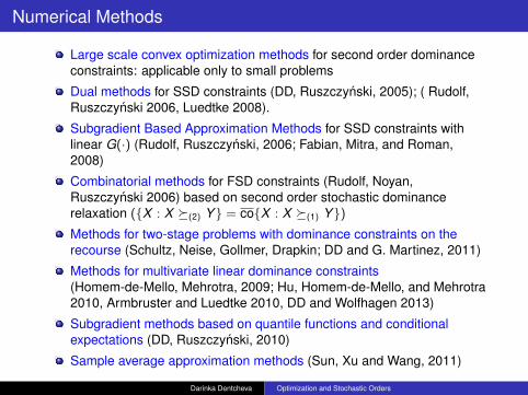
Numerical Methods

Large scale convex optimization methods for second order dominanceconstraints: applicable only to small problems

Dual methods for SSD constraints (DD, Ruszczynski, 2005); ( Rudolf,Ruszczynski 2006, Luedtke 2008).

Subgradient Based Approximation Methods for SSD constraints withlinear G(·) (Rudolf, Ruszczynski, 2006; Fabian, Mitra, and Roman,2008)

Combinatorial methods for FSD constraints (Rudolf, Noyan,Ruszczynski 2006) based on second order stochastic dominancerelaxation (X : X (2) Y = coX : X (1) Y)Methods for two-stage problems with dominance constraints on therecourse (Schultz, Neise, Gollmer, Drapkin; DD and G. Martinez, 2011)

Methods for multivariate linear dominance constraints(Homem-de-Mello, Mehrotra, 2009; Hu, Homem-de-Mello, and Mehrotra2010, Armbruster and Luedtke 2010, DD and Wolfhagen 2013)

Subgradient methods based on quantile functions and conditionalexpectations (DD, Ruszczynski, 2010)

Sample average approximation methods (Sun, Xu and Wang, 2011)


Extensions and Further Research Directions

Non-convex problems Optimality conditions for problems withFSD constraints and problems with higher order dominanceconstraints with non-convex functions (DD, A Ruszczynski 2004,2007)Stochastic dominance efficiency in multi-objective optimizationand its relations to dominance constraints (G. Mitra, C. Fabian,K. Darby-Dowman, D. Roman, 2006, 2009)Stability and sensitivity analysis, asymptotic behavior (DD, R.Henrion, A Ruszczynski, 2007; Y. Liu, H. Xu, 2010; DD and W. Römisch2011)

Semi-infinite composite optimization (DD, A Ruszczynski 2007)Robust Dominance Relation (DD, A Ruszczynski, 2010)


Applications

Finance: portfolio optimizationElectricity markets: portfolio of contracts and/or acceptability ofcontractsInverse models and forecasting: Compare the forecast errors viastochastic dominance and design data collection for modelcalibrationNetwork design: assign capacity to optimize network throughputRobotics: control of position and communication of robotsMedicine: radiation therapy designs


Optimization Problems with Stochastic Order …...Optimization Problems with Stochastic Order...

Documents

Transcript of Optimization Problems with Stochastic Order …...Optimization Problems with Stochastic Order...