Optimization of Noisy Functionspages.cs.wisc.edu/~Ferris/Talks/Informs-washington.pdfWISOPT...

Optimization of Noisy Functions

Geng Deng Michael C. Ferris

University of Wisconsin-Madison

INFORMS, October 15, 2008

Michael Ferris (University of Wisconsin) Simulation-Based Optimization INFORMS, 15 Oct 1 / 26

A general problem formulation

We formulate a noisy optimization problem as

minx∈S

f (x) = E[F (x , ξ(ω))],

ξ(ω) is a random component arising in some simulation process.

The sample response function F (x , ξ(ω))I typically does not have a closed form, thus cannot provide gradient or

Hessian informationI is normally computationally expensiveI is affected by uncertain factors in simulation

The underlying objective function f (x) has to be estimated.


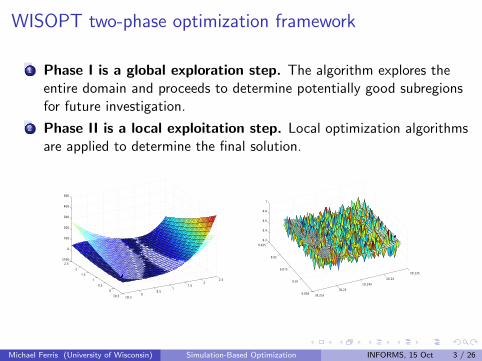
WISOPT two-phase optimization framework

1 Phase I is a global exploration step. The algorithm explores theentire domain and proceeds to determine potentially good subregionsfor future investigation.

2 Phase II is a local exploitation step. Local optimization algorithmsare applied to determine the final solution.

−0.50

0.51

1.52

2.5

−0.5

0

0.5

1

1.5

2

2.5−100

0

100

200

300

400

500

−0.255

−0.25

−0.245

−0.24

−0.235

0.005

0.01

0.015

0.02

0.025

0.2

0.4

0.6

0.8

1


The flow chart of WISOPT


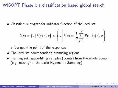
WISOPT Phase I: a classification based global search

Classifier: surrogate for indicator function of the level set

L(c) = {x f (x) ≤ c} '

x f̄ (x) =1

N

N∑j=1

F (x , ξj) ≤ c

c is a quantile point of the responses

The level set corresponds to promising regions

Training set: space-filling samples (points) from the whole domain(e.g. mesh grid; the Latin Hypercube Sampling)


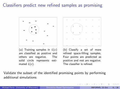
Classifiers predict new refined samples as promising

(a) Training samples in L(c)are classified as positive andothers are negative. Thesolid circle represents esti-mated L(c).

(b) Classify a set of morerefined space-filling samples.Four points are predicted aspositive and rest are negative.The classifier is refined.

Validate the subset of the identified promising points by performingadditional simulations


Imbalanced data

To identify the top promising regions, the best 10% of the trainingsamples are labeled as ‘+’, and the rest are ‘-’

The imbalance of the training set causes low classification accuracy,especially for positive members

Balance the training data setI Under-sample of the negative class using one-sided selection

F Use 1-NN and retain only those negative samples needed to predicttraining set

F Clean the dataset with Tomek links

I Over-sample of the positive class by duplicating positive samples

Adjust the misclassification penalty


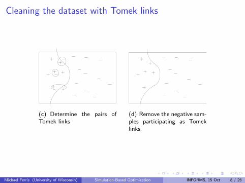
Cleaning the dataset with Tomek links

(c) Determine the pairs ofTomek links

(d) Remove the negative sam-ples participating as Tomeklinks


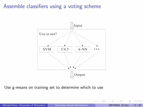
Assemble classifiers using a voting scheme

Use g-means on training set to determine which to use


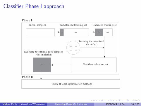
Classifier Phase I approach


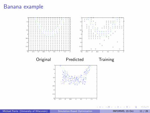
Banana example

−2 −1.5 −1 −0.5 0 0.5 1 1.5 2−2

−1.5

−1

−0.5

0

0.5

1

1.5

2

−−−−−−−−−−−−−−−−−−−−

−−−−−−−−−−−−−−−−−−−−

−−−−−−−−−−−−−−−−−−−−

−−−−−−−−−−−−−−−−−−

−−−−−−−−−−−−−−−

−−−

−−−−−−−−−−−−−

−−−−

−−−−−−−−−−−

−−−−−−

−−−−−−−−−−

−−−−−−−

−−−−−−−−−

−−−−−−−−

−−−−−−−−−

−−−−−−−−

−−−−−−−−−

−−−−−−−−

−−−−−−−−−

−−−−−−−−

−−−−−−−−−−

−−−−−−−

−−−−−−−−−−−

−−−−−−

−−−−−−−−−−−−−

−−−−

−−−−−−−−−−−−−−−

−−

−−−−−−−−−−−−−−−−−

−−−−−−−−−−−−−−−−−−−−

−−−−−−−−−−−−−−−−−−−−

−−−−−−−−−−−−−−−−−−−−

−2 −1.5 −1 −0.5 0 0.5 1 1.5 2−2

−1.5

−1

−0.5

0

0.5

1

1.5

2

−

−−

− −−

−

−

−−

−

−−

−

−

−

−

−

−

−−

−

−−−

−

−−−−−−−−

−−−−−−

−−−

−−−−

−

−−−

−−

−−

− −−

−

−−−−−

−−

−−−−−

−−

−

−−

−−

−−

−−−−−−−

−−

−

Original Predicted Training

−2 −1.5 −1 −0.5 0 0.5 1 1.5 2−2

−1.5

−1

−0.5

0

0.5

1

1.5

2


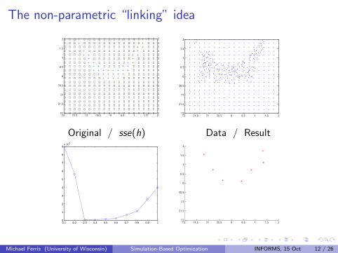
The non-parametric “linking” idea

−2 −1.5 −1 −0.5 0 0.5 1 1.5 2−2

−1.5

−1

−0.5

0

0.5

1

1.5

2

−−−−−−−−−−−−−−−−−−−−

−−−−−−−−−−−−−−−−−−−−

−−−−−−−−−−−−−−−−−−−−

−−−−−−−−−−−−−−−−−−

−−−−−−−−−−−−−−−

−−−

−−−−−−−−−−−−−

−−−−

−−−−−−−−−−−

−−−−−−

−−−−−−−−−−

−−−−−−−

−−−−−−−−−

−−−−−−−−

−−−−−−−−−

−−−−−−−−

−−−−−−−−−

−−−−−−−−

−−−−−−−−−

−−−−−−−−

−−−−−−−−−−

−−−−−−−

−−−−−−−−−−−

−−−−−−

−−−−−−−−−−−−−

−−−−

−−−−−−−−−−−−−−−

−−

−−−−−−−−−−−−−−−−−

−−−−−−−−−−−−−−−−−−−−

−−−−−−−−−−−−−−−−−−−−

−−−−−−−−−−−−−−−−−−−−

−2 −1.5 −1 −0.5 0 0.5 1 1.5 2−2

−1.5

−1

−0.5

0

0.5

1

1.5

2

Original / sse(h) Data / Result

0.1 0.2 0.3 0.4 0.5 0.6 0.7 0.8 0.9 10

1

2

3

4

5

6

7

8

9x 10

4

−2 −1.5 −1 −0.5 0 0.5 1 1.5 2−2

−1.5

−1

−0.5

0

0.5

1

1.5

2


Determine subregion radius by non-parametric regression

The idea is to determine the best ‘window size’ for non-parametric localquadratic regression

1 ∆ ∈ arg minh sse(h)

2 sse(h) is the sum of squared error of knock-one out prediction. Givena window-size h and a point y , the knock-one out predicted value isQy

h (y), where Qyh (x) is a quadratic regression function constructed

using the data points within the ball {x | ‖x − y‖ ≤ h}/{y}.

Qyh (x) = c + gT (x − y) +

1

2(x − y)TH(x − y)

.


Phase II: refine solution

Local optimization methods to handle noise

Derivative-free methods

Basic approach: reduce function uncertainty by averaging multiplesamples per point.

Potential difficulty:efficiency of algorithm vs number of simulation runs

We apply Bayesian approach to determine appropriate number ofsamples per point, while simultaneously enhancing the algorithmefficiency


Quadratic model construction and trust region subproblemsolution

For iteration k = 1, 2, . . .,

· · ·Construct a quadratic model via interpolation

Q(x , ξ) = F (xk , ξ) + gTQ (ξ)(x − xk) +

1

2(x − xk)TGQ(ξ)(x − xk)

The model is unstable since interpolating noisy data

Solve the trust region subproblem

s∗k (ξ) = arg mins Q(xk + s, ξ)s.t. ‖s‖2 ≤ ∆k

The solution is thus unstable

· · ·


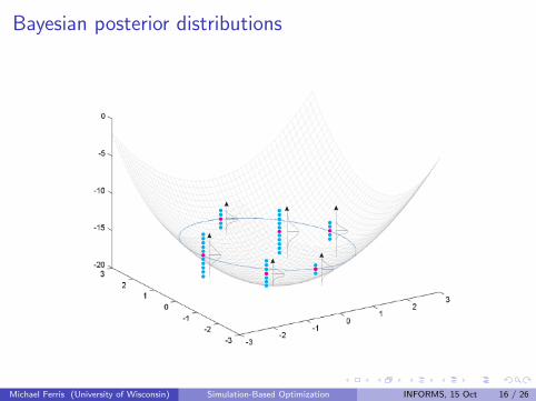
Bayesian posterior distributions


Constraining the variance of solutions (Monte Carlovalidation)

Generate ‘sample quadratic functions’ that could arise given currentfunction evaluations.

Trial solutions are generated within a trust region. The standarddeviation of the solutions are constrained.

nmaxi=1

std([s∗(1)(i), s∗(2)(i), · · · , s∗(M)(i)]) ≤ β∆k .


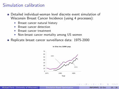
Simulation calibration

Detailed individual-woman level discrete event simulation ofWisconsin Breast Cancer Incidence (using 4 processes):

I Breast cancer natural historyI Breast cancer detectionI Breast cancer treatmentI Non-breast cancer mortality among US women

Replicate breast cancer surveillance data: 1975-2000

In Situ Inc./100K pop.

0

10

20

30

40

50

60

70

1975 1985 1995

Year

SEER

WCRS


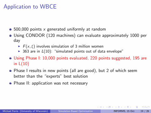
Application to WBCE

500,000 points x generated uniformly at random

Using CONDOR (120 machines) can evaluate approximately 1000 perday

I F (x , ξ) involves simulation of 3 million womenI 363 are in L(10): “simulated points out of data envelope”

Using Phase I: 10,000 points evaluated, 220 points suggested, 195 arein L(10)

Phase I results in new points (all are good), but 2 of which seembetter than the “experts” best solution

Phase II: application was not necessary


Design a coaxial antenna for hepatic tumor ablation


Simulation of the electromagnetic radiation profile

Finite element models (COMSOL MultiPhysics v3.2) are used to generatethe electromagnetic (EM) radiation fields in liver given a particular design

Metric Measure of Goal

Lesion radius Size of lesion in radial direction MaximizeAxial ratio Proximity of lesion shape to a sphere Fit to 0.5S11 Tail reflection of antenna Minimize


Two-phase approach to optimize antenna designparameters

Uniform LHS to generate 1,000 design samples to evaluate with theFE simulation model (range [-0.1409, 0.2903])

c = −0.0354 the 10% quantile. L(c) has 100 positive samples (900negative)

Balancing procedure: 200 positive vs. 269 negative samples

3 (of 6 tested using g-means) classifiers in ensemble

Refined data: 20,000 designs, 1914 predicted by classifiers as positive,74.5% correctly

The best Phase I design has value -0.2238


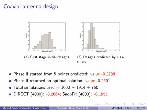
Coaxial antenna design

−0.4 −0.35 −0.3 −0.25 −0.2 −0.15 −0.1 −0.05 00

5

10

15

20

25

30

Objective Value

Per

cent

(e) First stage initial designs

−0.4 −0.35 −0.3 −0.25 −0.2 −0.15 −0.1 −0.05 00

5

10

15

20

25

30

Objective Value

Per

cent

(f) Designs predicted by clas-sifiers

Phase II started from 5 points predicted: value -0.2238

Phase II returned an optimal solution: value -0.2501

Total simulations used = 1000 + 1914 + 750

DIRECT (4000): -0.2064; SnobFit (4000): -0.1955


Noisy extension: changing liver properties

Dielectric tissue properties varied within ±10% of average propertiesto simulate the individual variation.

WISOPT yields an optimal design that is a 27.3% improvement overthe original design and is more robust in terms of lesion shape andefficiency.


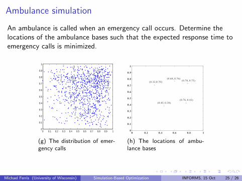
Ambulance simulation

An ambulance is called when an emergency call occurs. Determine thelocations of the ambulance bases such that the expected response time toemergency calls is minimized.

0 0.1 0.2 0.3 0.4 0.5 0.6 0.7 0.8 0.9 10

0.1

0.2

0.3

0.4

0.5

0.6

0.7

0.8

0.9

1

(g) The distribution of emer-gency calls

(h) The locations of ambu-lance bases


Conclusions and future work

Coupling statistical and optimization techniques can effectivelyprocess noisy function optimizations

Significant gains in system performance and robustness are possible

WISOPT framework allows multiple methods to be “hooked” up

Future work:

Problems with general constraints

More optimization algorithms in both phases

A phase transition module with variable radii


Optimization of Noisy Functionspages.cs.wisc.edu/~Ferris/Talks/Informs-washington.pdfWISOPT...

Documents

Transcript of Optimization of Noisy Functionspages.cs.wisc.edu/~Ferris/Talks/Informs-washington.pdfWISOPT...