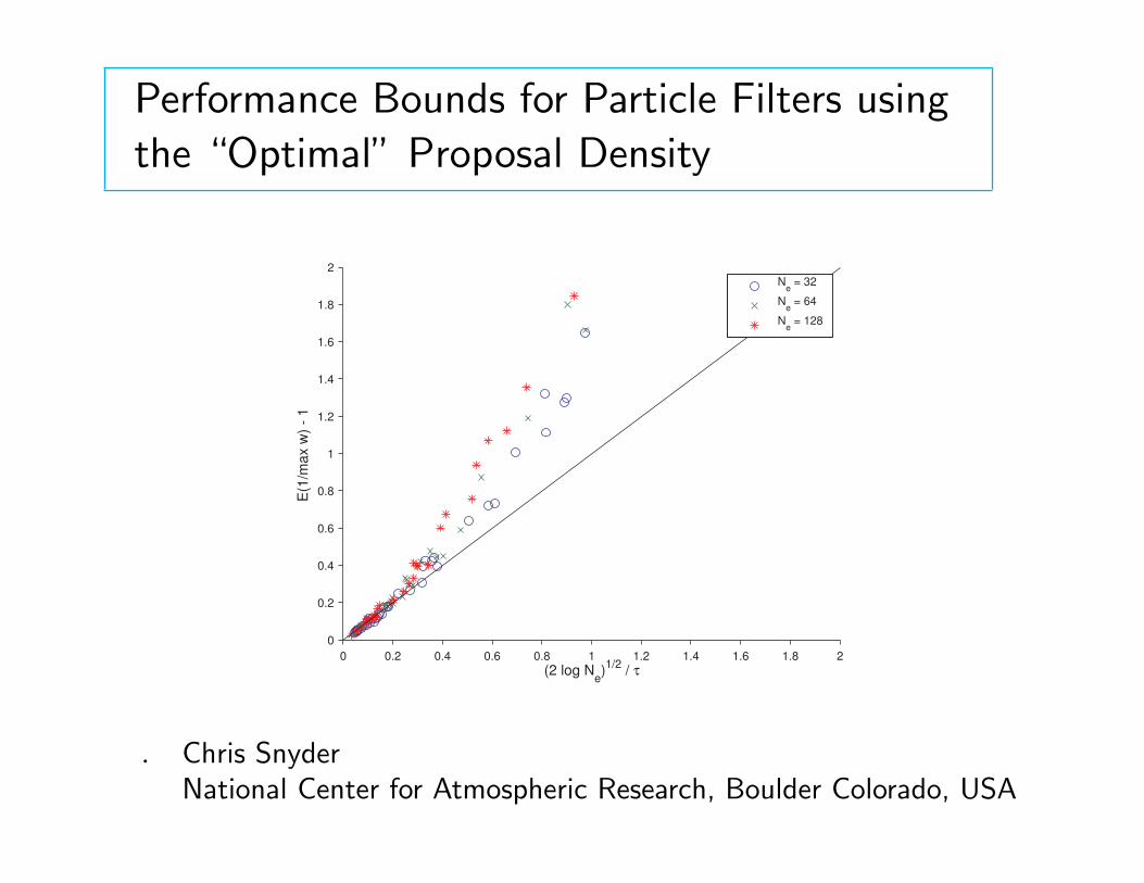
Performance Bounds for Particle Filters using

the “Optimal” Proposal Density

0 0.2 0.4 0.6 0.8 1 1.2 1.4 1.6 1.8 2

0

0.2

0.4

0.6

0.8

1

1.2

1.4

1.6

1.8

2

(2 log Ne)1/2

/ τ

E(1

/ma

x w

) -

1

N

e = 32

Ne = 64

Ne = 128

. Chris SnyderNational Center for Atmospheric Research, Boulder Colorado, USA

1

Overview

. Simplest particle filter requires very large ensemble size, growingexponentially with the problem size.

. Can the use of the optimal proposal density fix this?

2

Preliminaries

Notation

. follow Ide et al. (1997) generally, except:. . . dim(x) = Nx, dim(y) = Ny, ensemble size = Ne

. . . superscripts index ensemble members

. ∼ means “distributed as,” e.g. x ∼ N(0, 1). Also used for“asymptotic to”

. state evolution: xk =M(xk−1) + ηk

. observations: yk = H(xk) + εk

Interchangeable terms

. particles ≡ ensemble members

. sample ≡ ensemble

3

Preliminaries: The Simplest Particle Filter

. begin with members xik−1 and weights wik−1 that “represent”

p(xk−1|yok−1)

. compute xik by evolving each member to tk under the system dynamics

. re-weight, given new obs yok: wik ∝ wi

k−1p(yok|xik)

. (resample)

4

Preliminaries: Sequential Importance Sampling

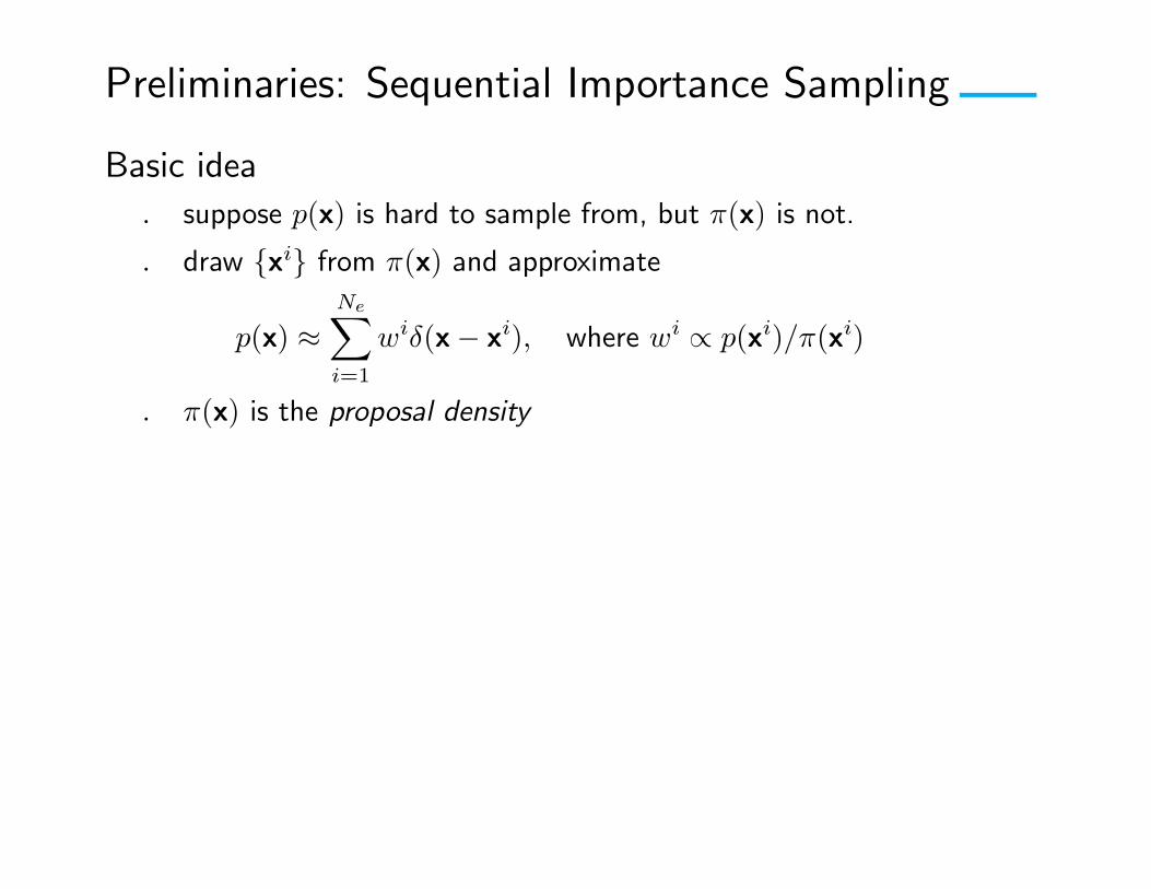
Basic idea

. suppose p(x) is hard to sample from, but π(x) is not.

. draw {xi} from π(x) and approximate

p(x) ≈Ne∑i=1

wiδ(x− xi), where wi ∝ p(xi)/π(xi)

. π(x) is the proposal density

5

Preliminaries: SIS (cont.)

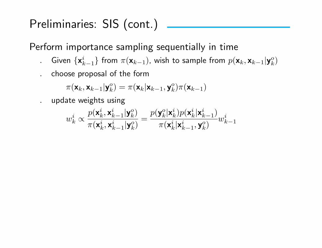
Perform importance sampling sequentially in time

. Given {xik−1} from π(xk−1), wish to sample from p(xk, xk−1|yok)

. choose proposal of the form

π(xk, xk−1|yok) = π(xk|xk−1, yok)π(xk−1)

. update weights using

wik ∝

p(xik, xik−1|yok)

π(xik, xik−1|yok)

=p(yok|xik)p(xik|xik−1)

π(xik|xik−1, yok)

wik−1

6

Preliminaries: SIS (cont.)

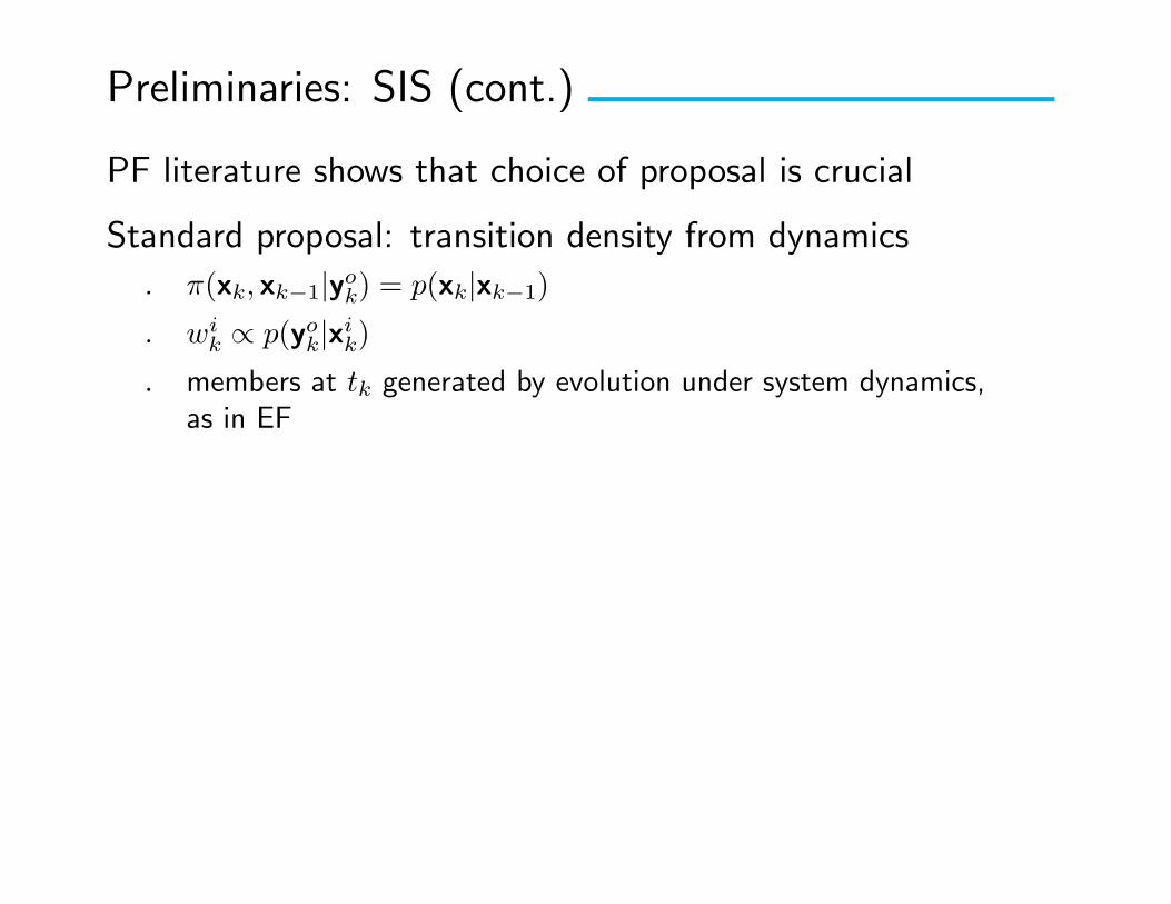
PF literature shows that choice of proposal is crucial

Standard proposal: transition density from dynamics

. π(xk, xk−1|yok) = p(xk|xk−1)

. wik ∝ p(yok|xik)

. members at tk generated by evolution under system dynamics,as in EF

7

Preliminaries: SIS (cont.)

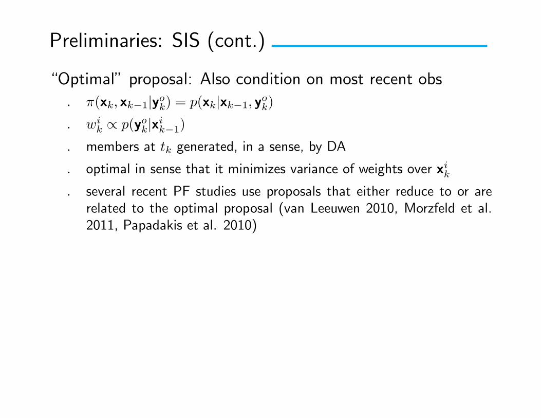
“Optimal” proposal: Also condition on most recent obs

. π(xk, xk−1|yok) = p(xk|xk−1, yok)

. wik ∝ p(yok|xik−1)

. members at tk generated, in a sense, by DA

. optimal in sense that it minimizes variance of weights over xik

. several recent PF studies use proposals that either reduce to or arerelated to the optimal proposal (van Leeuwen 2010, Morzfeld et al.2011, Papadakis et al. 2010)

8

Degeneracy of PF Weights

. degeneracy ≡ maxiwik → 1

. common problem, well known in PF literature

. for standard proposal, Bengtsson et al. (2008) and Snyder et al.(2008) show Ne must increase exponentially as problem size increasesin order to avoid degeneracy

. What happens with optimal proposal?

9

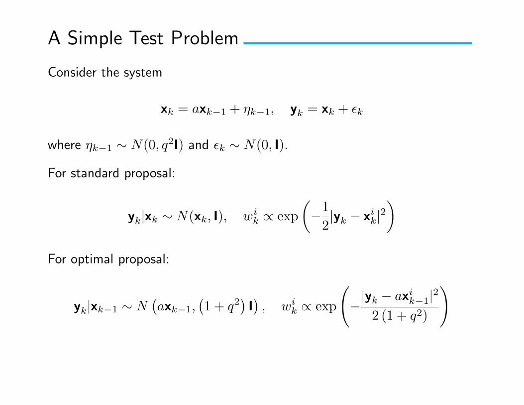
A Simple Test Problem

Consider the system

xk = axk−1 + ηk−1, yk = xk + εk

where ηk−1 ∼ N(0, q2I) and εk ∼ N(0, I).

For standard proposal:

yk|xk ∼ N(xk, I), wik ∝ exp

(−12|yk − xik|2

)For optimal proposal:

yk|xk−1 ∼ N(axk−1,

(1 + q2

)I), wi

k ∝ exp

(−|yk − axik−1|2

2 (1 + q2)

)

10

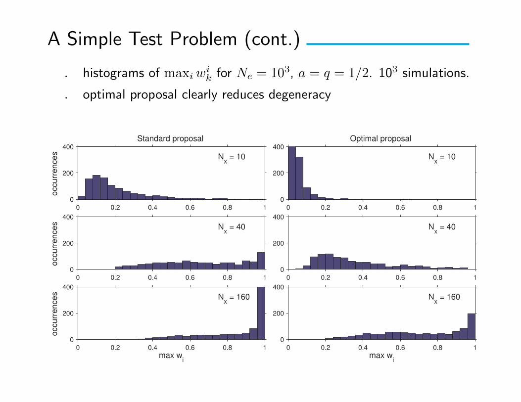
A Simple Test Problem (cont.)

. histograms of maxiwik for Ne = 103, a = q = 1/2. 103 simulations.

. optimal proposal clearly reduces degeneracy

0 0.2 0.4 0.6 0.8 10

200

400

max wi

occurr

ences N

x = 160

0 0.2 0.4 0.6 0.8 10

200

400

max wi

Nx = 160

0 0.2 0.4 0.6 0.8 10

200

400

occurr

ences N

x = 40

0 0.2 0.4 0.6 0.8 10

200

400

Nx = 40

0 0.2 0.4 0.6 0.8 10

200

400

occurr

ences N

x = 10

Standard proposal

0 0.2 0.4 0.6 0.8 10

200

400

Nx = 10

Optimal proposal

11

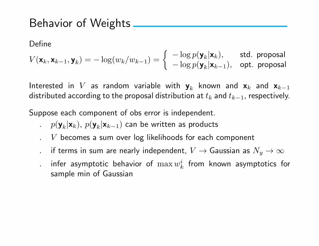
Behavior of Weights

Define

V (xk, xk−1, yk) = − log(wk/wk−1) =

{− log p(yk|xk), std. proposal− log p(yk|xk−1), opt. proposal

Interested in V as random variable with yk known and xk and xk−1

distributed according to the proposal distribution at tk and tk−1, respectively.

Suppose each component of obs error is independent.

. p(yk|xk), p(yk|xk−1) can be written as products

. V becomes a sum over log likelihoods for each component

. if terms in sum are nearly independent, V → Gaussian as Ny →∞

. infer asymptotic behavior of maxwik from known asymptotics for

sample min of Gaussian

12

Behavior of Weights (cont.)

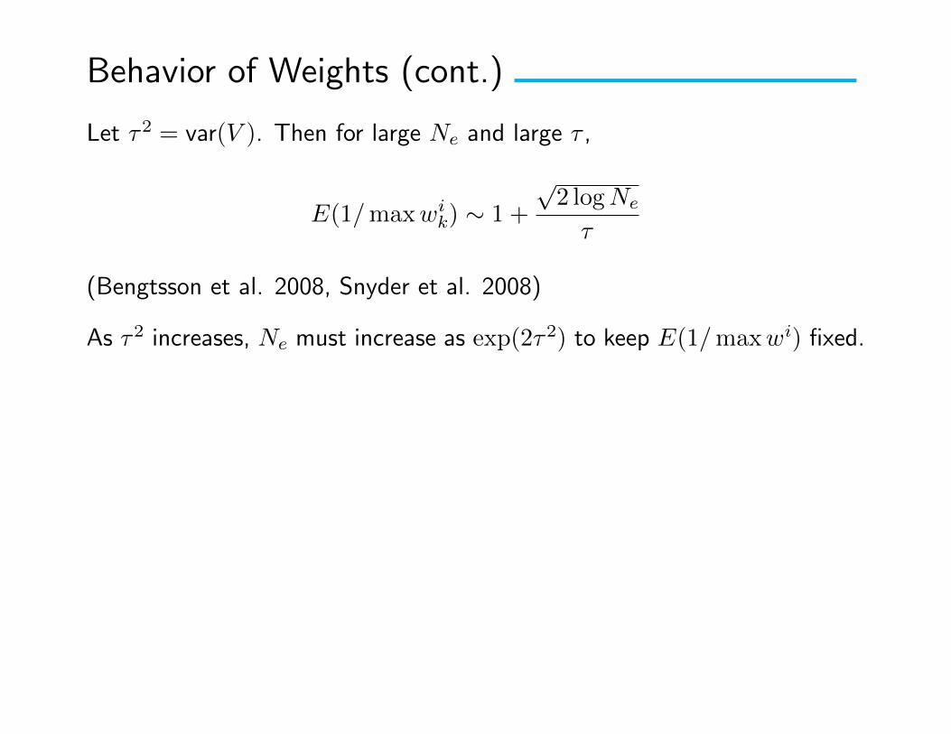
Let τ2 = var(V ). Then for large Ne and large τ ,

E(1/maxwik) ∼ 1 +

√2 logNe

τ

(Bengtsson et al. 2008, Snyder et al. 2008)

As τ2 increases, Ne must increase as exp(2τ2) to keep E(1/maxwi) fixed.

13

The Linear, Gaussian Case

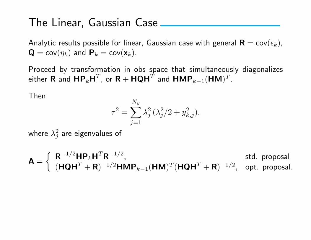
Analytic results possible for linear, Gaussian case with general R = cov(εk),Q = cov(ηk) and Pk = cov(xk).

Proceed by transformation in obs space that simultaneously diagonalizeseither R and HPkH

T , or R+HQHT and HMPk−1(HM)T .

Then

τ2 =

Ny∑j=1

λ2j (λ2j/2 + y2k,j),

where λ2j are eigenvalues of

A =

{R−1/2HPkH

TR−1/2, std. proposal

(HQHT + R)−1/2HMPk−1(HM)T (HQHT + R)−1/2, opt. proposal.

14

Simple Test Problem, Revisited

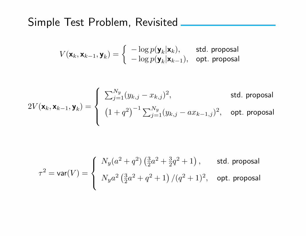
V (xk, xk−1, yk) =

{− log p(yk|xk), std. proposal− log p(yk|xk−1), opt. proposal

2V (xk, xk−1, yk) =

∑Ny

j=1(yk,j − xk,j)2, std. proposal(1 + q2

)−1∑Ny

j=1(yk,j − axk−1,j)2, opt. proposal

τ2 = var(V ) =

Ny(a

2 + q2)(32a

2 + 32q

2 + 1), std. proposal

Nya2(32a

2 + q2 + 1)/(q2 + 1)2, opt. proposal

15

Simple Test Problem, Revisited (cont.)

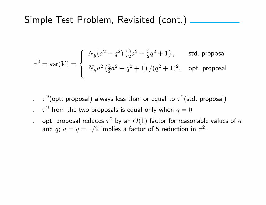
τ2 = var(V ) =

Ny(a

2 + q2)(32a

2 + 32q

2 + 1), std. proposal

Nya2(32a

2 + q2 + 1)/(q2 + 1)2, opt. proposal

. τ2(opt. proposal) always less than or equal to τ2(std. proposal)

. τ2 from the two proposals is equal only when q = 0

. opt. proposal reduces τ2 by an O(1) factor for reasonable values of aand q; a = q = 1/2 implies a factor of 5 reduction in τ2.

16

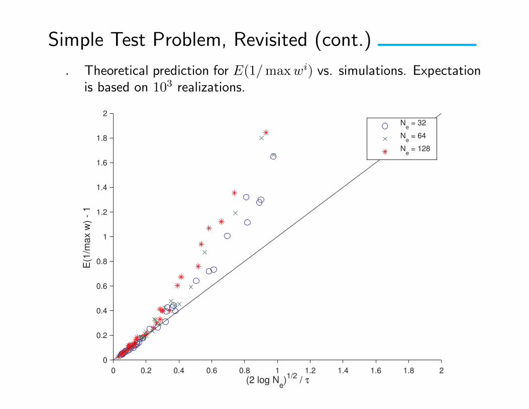
Simple Test Problem, Revisited (cont.)

. Theoretical prediction for E(1/maxwi) vs. simulations. Expectationis based on 103 realizations.

0 0.2 0.4 0.6 0.8 1 1.2 1.4 1.6 1.8 2

0

0.2

0.4

0.6

0.8

1

1.2

1.4

1.6

1.8

2

(2 log Ne)1/2

/ τ

E(1

/ma

x w

) -

1

N

e = 32

Ne = 64

Ne = 128

17

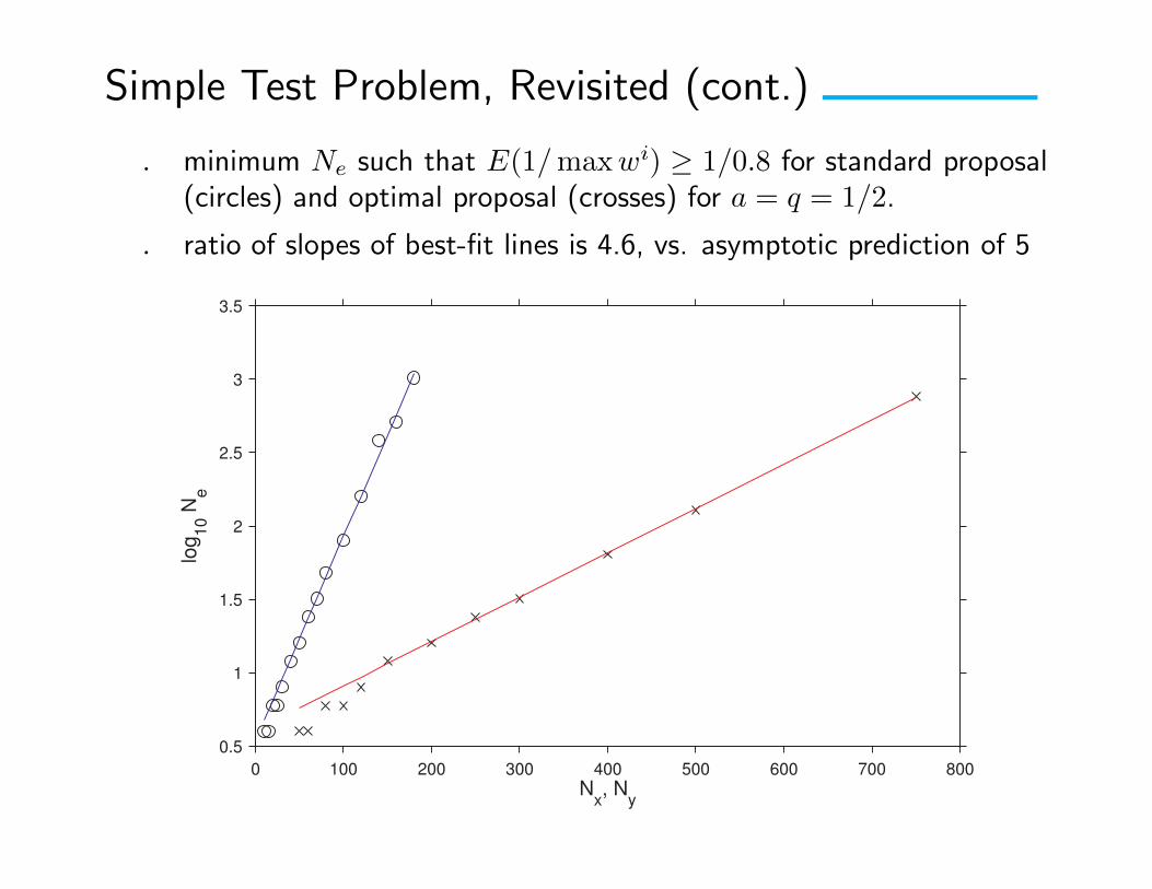
Simple Test Problem, Revisited (cont.)

. minimum Ne such that E(1/maxwi) ≥ 1/0.8 for standard proposal(circles) and optimal proposal (crosses) for a = q = 1/2.

. ratio of slopes of best-fit lines is 4.6, vs. asymptotic prediction of 5

0 100 200 300 400 500 600 700 800

0.5

1

1.5

2

2.5

3

3.5

Nx, N

y

log

10 N

e

18

Ny, Nx and Problem Size

τ2 = var(log likelihood) measures “problem size” for PF

. as τ2 increases, Ne must increase as exp(2τ2) if E(1/maxwi) fixed.

Related to obs-space dimension

. in simple example, τ2 ∝ Ny

. given by sum over e-values of obs-space covariance in general linear,Gaussian case—like an effective dimension

Analogy of τ2 to dimension is incomplete

. τ2 depends on obs-error statistics, increasing as R decreases

. τ2 depends on proposal

19

Ny, Nx and Problem Size (cont.)

τ2 depends explicitly only on obs-space quantities

How does Nx affect weight degeneracy?

. asymptotic relation of τ2 and E(1/maxwi) requires V (xk, xk−1, yk)to be ∼ Gaussian over xk

. ∼ Gaussianity of V (xk) only if Nx = dim(x) is large and componentsof x are sufficiently independent

20

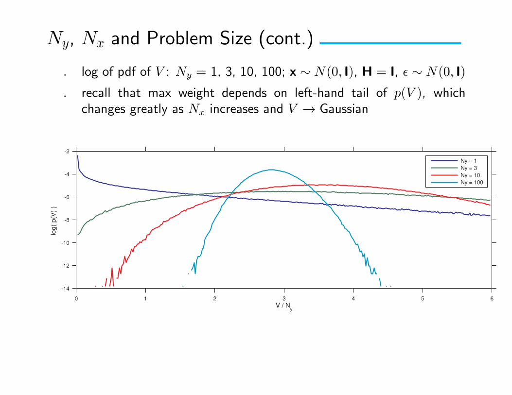
Ny, Nx and Problem Size (cont.)

. log of pdf of V : Ny = 1, 3, 10, 100; x ∼ N(0, I), H = I, ε ∼ N(0, I)

. recall that max weight depends on left-hand tail of p(V ), whichchanges greatly as Nx increases and V → Gaussian

0 1 2 3 4 5 6

-14

-12

-10

-8

-6

-4

-2

V / Ny

log(

p(V

) )

Ny = 1

Ny = 3

Ny = 10

Ny = 100

21

Summary

. As was the case for the standard proposal, the optimal proposalrequires Ne to increase exponentially with the “problem size” toavoid degeneracy.

. Exponential rate of increase is quantitatively smaller for the optimalproposal; necessary ensemble size may therefore be much smaller ina given problem.

. Benefits of optimal proposal dependent on magnitude of system noise.

. (In some cases, possible to enhance performance of optimal proposalby artificially increasing system noise in forecast model used infiltering.)

22

Recommendation

New PF algorithms intended for high-dimensional systems should beevaluated first on the simple test problem given here.

23

References

Bengtsson, T., P. Bickel and B. Li, 2008: Curse-of-dimensionality revisited: Collapse of the particle filter invery large scale systems. IMS Collections, 2, 316–334. doi: 10.1214/193940307000000518.

Morzfeld, M., X. Tu, E. Atkins and A. J. Chorin, 2011: A random map implementation of implicit filters. J.

Comput. Phys. 231, 2049–2066.

van Leeuwen, P. J., 2010: Nonlinear data assimilation in geosciences: an extremely efficient particle filter.Quart. J. Roy. Meteor. Soc. 136, 1991–1999.

Papadakis, N., E. Memin, A. Cuzol and N. Gengembre, 2010: Data assimilation with the weighted ensembleKalman filter. Tellus 62A, 673–697.

Snyder, C., T. Bengtsson, P. Bickel and J. Anderson, 2008: Obstacles to high-dimensional particle filtering.Monthly Wea. Rev., 136, 4629–4640.

24