Optimal Brownian stopping when the source and target are ...
29
OPTIMAL BROWNIAN STOPPING WHEN THE SOURCE AND TARGET ARE RADIALLY SYMMETRIC DISTRIBUTIONS By Nassif Ghoussoub † Young-Heon Kim † and Tongseok Lim ‡ The University of British Columbia † and ShanghaiTech University ‡ Given two probability measures μ, ν on R d , in subharmonic or- der, we describe optimal stopping times τ that maximize/minimize the cost functional E|B0 - Bτ | α , α> 0, where (Bt )t is Brownian motion with initial law μ and with final distribution –once stopped at τ – equal to ν . Under the assumption of radial symmetry on μ and ν , we show that in dimension d ≥ 3 and α 6= 2, there exists a unique optimal solution given by a non-randomized stopping time characterized as the hitting time to a suitably symmetric barrier. We also relate this problem to the optimal transportation problem for subharmonic martingales, and establish a duality result. This paper is an expanded version of a previously posted but not published work by the authors [22]. 1. Introduction. Let μ and ν be two probability measures on R d , d ≥ 2 with finite first moment, and let (B t ) t denote the Brownian motion with initial law μ. We consider the following –possibly empty– set of stopping times, with respect to the Brownian filtration: T (μ, ν )= {τ | τ is a stopping time, B 0 ∼ μ, B τ ∼ ν, and E[τ ] < ∞}, where here and in the sequel, the notation X ∼ λ means that the law of the random variable X is the probability measure λ. For a given cost function c : R d × R d → R, and assuming T (μ, ν ) is non-empty, we shall consider the following optimization problem Maximize / Minimize E [c(B 0 ,B τ )] over τ ∈T (μ, ν ). (1.1) * The first two authors are partially supported by the Natural Sciences and Engineering Research Council of Canada (NSERC). Y.-H. Kim was also supported by an Alfred P. Sloan Research Fellow- ship. T. Lim was partly supported by a doctoral graduate fellowship from the University of British Columbia, by the Austrian Science Foundation (FWF) through grant Y782, and by the European Research Council under the European Union’s Seventh Framework Programme (FP7/2007-2013) / ERC grant agreement no. 335421. In addition, T. Lim gratefully acknowledges support from ShanghaiTech University. Part of this research was done while the authors were visiting the Fields institute in Toronto during the thematic program on “Calculus of Variations” in Fall 2014. We are thankful for the hospitality and the great research environment that the institute provided. MSC 2010 subject classifications: Primary 49-XX, 60-XX; secondary 52-XX Keywords and phrases: Subharmonic Martingale Optimal Transport, Skorokhod Embedding, Monotonicity, Radial Symmetry. 1
Transcript of Optimal Brownian stopping when the source and target are ...
OPTIMAL BROWNIAN STOPPING WHEN THE SOURCE ANDTARGET ARE RADIALLY SYMMETRIC DISTRIBUTIONS
By Nassif Ghoussoub† Young-Heon Kim† and Tongseok Lim‡
The University of British Columbia† and ShanghaiTech University ‡
Given two probability measures µ, ν on Rd, in subharmonic or-der, we describe optimal stopping times τ that maximize/minimizethe cost functional E|B0 − Bτ |α, α > 0, where (Bt)t is Brownianmotion with initial law µ and with final distribution –once stoppedat τ– equal to ν. Under the assumption of radial symmetry on µand ν, we show that in dimension d ≥ 3 and α 6= 2, there existsa unique optimal solution given by a non-randomized stopping timecharacterized as the hitting time to a suitably symmetric barrier. Wealso relate this problem to the optimal transportation problem forsubharmonic martingales, and establish a duality result. This paperis an expanded version of a previously posted but not published workby the authors [22].
1. Introduction. Let µ and ν be two probability measures on Rd, d ≥ 2 withfinite first moment, and let (Bt)t denote the Brownian motion with initial law µ. Weconsider the following –possibly empty– set of stopping times, with respect to theBrownian filtration:
T (µ, ν) = τ | τ is a stopping time, B0 ∼ µ,Bτ ∼ ν, and E[τ ] <∞,
where here and in the sequel, the notation X ∼ λ means that the law of the randomvariable X is the probability measure λ.
For a given cost function c : Rd×Rd → R, and assuming T (µ, ν) is non-empty, weshall consider the following optimization problem
Maximize / Minimize E [c(B0, Bτ )] over τ ∈ T (µ, ν).(1.1)
∗The first two authors are partially supported by the Natural Sciences and Engineering ResearchCouncil of Canada (NSERC). Y.-H. Kim was also supported by an Alfred P. Sloan Research Fellow-ship. T. Lim was partly supported by a doctoral graduate fellowship from the University of BritishColumbia, by the Austrian Science Foundation (FWF) through grant Y782, and by the EuropeanResearch Council under the European Union’s Seventh Framework Programme (FP7/2007-2013)/ ERC grant agreement no. 335421. In addition, T. Lim gratefully acknowledges support fromShanghaiTech University. Part of this research was done while the authors were visiting the Fieldsinstitute in Toronto during the thematic program on “Calculus of Variations” in Fall 2014. We arethankful for the hospitality and the great research environment that the institute provided.
MSC 2010 subject classifications: Primary 49-XX, 60-XX; secondary 52-XXKeywords and phrases: Subharmonic Martingale Optimal Transport, Skorokhod Embedding,
Monotonicity, Radial Symmetry.
1
2 N. GHOUSSOUB, Y-H KIM AND T. LIM
Recall that a stopping time on a filtered probability space (Ω,F , (Ft)t,P) is arandom variable τ : Ω → [0,+∞] such that τ ≤ t ∈ Ft for every t ≥ 0. Arandomized stopping time is a probability measure τ on Ω × [0,+∞] such that foreach u ∈ R+, the random time ρu(ω) := inft ≥ 0 : τω([0, t]) ≥ u is a stoppingtime, where (τω)ω is a disintegration of τ along the path ω according to P, that isτ(dω, dt) = τω(dt)P(dω). In the sequel, “stopping times” including those in T (µ, ν),will mean possibly randomized stopping times unless stated otherwise. We note thata stopping time is non-randomized if the disintegration τω is the Dirac measure on R+
for P a.e. ω. For further details See Section 2, and also e.g. Beiglbock-Cox-Huesmann[2], Guo-Tan-Touzi [26].
The purpose of the present article is to identify and characterize those optimal stop-ping times for which (1.1) is attained. In particular, we will be investigating whenoptimal stopping times are unique, ‘true’ as opposed to randomized, and whetherthey are hitting times of some barriers. Moreover, we consider how conditions of ra-dial symmetry on the source and target measures are reflected in terms of symmetryin the geometry of the barrier.
But first, we recall that the Skorokhod Embedding Problem (SEP) -initiated bySkorokhod [40] in the early 1960s- gives necessary and sufficient condition on apair (µ, ν), which insures that the set T (µ, ν) is non-empty. In dimension one, thiscondition states that µ and ν should be in convex order, that is
(1.2)∫fdµ ≤
∫fdν for every convex function f on Rd.
Since then, the problem and its variants were investigated by a large number ofresearchers, and have led to several important results in probability theory andstochastic processes. We refer to Ob loj [36] for an excellent survey of the subject,which describes no less than 21 different solutions to (SEP).
More recently, Hobson [27] made the connection between SEP and problems of ro-bust pricing and hedging of financial instruments. Hobson-Klimmek [29] and Hobson-Neuberger [30] connected SEP to finding robust price bounds for the forward startingstraddle. See the excellent survey of Hobson [28].
The interest eventually shifted to the problem of finding optimal solutions amongthose that solve (SEP). In other words, which among the stopping times in T (µ, ν)maximize or minimize a given cost function. Among the multitude of contributionsto these questions, we point out the papers of Beiglbock-Cox-Huesmann [2], Cox-Ob loj-Touzi [11], Dolinsky-Soner [13, 14], Guo-Tan-Touzi [26], Kallblad-Tan-Touzi[32], to name just a few. We do single out, however, the recent work of Beiglbock-Cox-Huesmann [2], which uses the analogy between the optimal SEP and the theoryof optimal mass transport, to identify and prove the so-called Monotonicity Principle(MP), which will be one of the main tools used in this paper.
Most of the previously mentioned works focus on the one-dimensional case. Morerecently, Ghoussoub-Kim-Palmer use dynamic programming and PDE methods to
OPTIMAL BROWNIAN STOPPING 3
give solutions, that is, optimal non-randomized stopping times, in all dimensions forthe minimization case when the cost is either c(x, y) = |x− y| or when it is dynamicand given by a certain Lagrangian [23, 24]. Left open is the case of a general cost,including those of the form
c(x, y) = |x− y|α,(1.3)
where 0 < α 6= 2, or more generally cost functions of the form c(x, y) = f(|x − y|),where f : R+ → R is a continuous function such that f(0) = 0.
The present paper also deals with higher dimensional situation, but with a focuson the case where both source and target measures are radially symmetric. One ofthe main goals is to analyze how this symmetry impacts the structure of the barriersets, whose hitting times determine the optimal stopping times. To state our firstmain result, we shall denote by Pc(O) the set of compactly supported probabilitymeasures whose supports are in a given open set O of Rd.
Theorem 1.1. Consider the cost function c(x, y) = |x − y|α, where 0 < α 6= 2,and let µ, ν ∈ Pc(Rd) be radial1, d ≥ 3 are such that T (µ, ν) is nonempty. Assumeµ ∈ H−1(Rd), µ ∧ ν = 0, µ(0) = 0, and µ(∂ suppµ) = 0.
Then, there exists a unique solution τ for the minimization/maximization problem(1.1), that is given by a non-randomized stopping time.
Moreover, in the minimization problem with 0 < α ≤ 1, the solution τ is stillunique also among all possibly randomized solutions, and without the assumptionthat µ ∧ ν = 0
Actually, we shall show that the optimal τ is a hitting time of a suitable barrier.Moreover, each barrier set for the Brownian motion Bx starting from x is axiallysymmetric around the line that connects the origin and x (see Remark 2.12). A sim-ilar structure is detected in the two dimensional case, however, it was not sufficientto yield a non-randomized stopping time (see Remark 2.13).
For the rest of this introduction, we do not assume that µ, ν are necessarily radial,but we shall need the notion of measures in subharmonic order. Recall that a functionf is subharmonic on an open set U in Rd if it is upper-semicontinuous with valueson R ∪ −∞ and satisfies
f(x) ≤ 1
Leb(B)
∫Bf(y)dy for every closed ball B in U with center at x.
When f is C2, the latter condition is equivalent to ∆f ≥ 0 on U , where ∆ =∑d
i=1∂∂xi
is the Laplacian. We note that, unlike convex functions, a subharmonic function onU may not have any subharmonic extension on a larger domain V . Therefore it is
1A measure µ is radial if µ(A) = µ(M(A)) for any A ∈ B(Rd) and any orthogonal matrix M .An example is the Gaussian measure with mean 0 and covariance matrix σ2 Id, σ > 0.
4 N. GHOUSSOUB, Y-H KIM AND T. LIM
important to specify a subharmonic function with its domain. We shall thereforeconsider SH(O) to be the cone of all subharmonic functions on an open set O.
Definition 1.2. We say that µ, ν ∈ Pc(Rd) are in subharmonic order if thefollowing holds:
(1.4)
∫f dµ ≤
∫f dν for every f ∈ SH(O),
where O is an open set containing supp(µ+ ν). We shall then write µ ≺s ν.
The fact that in higher dimension, the condition µ ≺s ν is also sufficient forthe non-emptiness of T (µ, ν) has been the subject of many studies. See for exampleRost [39], Monroe [35], Baxter-Chacon [1], Chacon-Walsh [9], Falkner [17] and manyothers. We shall give yet another proof of this fact from a different viewpoint, andpresent the intimate connection between the optimal Skorokhod embedding problem(OSEP) and the subharmonic martingale optimal transport (SMOT) problem thatwe now introduce.
For this, recall the martingale optimal transport (MOT) problem. Let Π(µ, ν) bethe set of transport plans with marginals µ, ν, i.e. the subset of P(Rd×Rd) consistingof all couplings of µ, ν (see [42]). Then the MOT problem consists of the following:
Minimize Cost[π] =
∫∫c(x, y)dπ(x, y) over π ∈ MT(µ, ν),(1.5)
where MT(µ, ν) is the set of martingale transport plans, that is, the subset of Π(µ, ν)such that for each π ∈ MT(µ, ν), its disintegration (πx)x∈Rd w.r.t. µ satisfies
f(x) ≤∫f(y) dπx(y)(1.6)
for any convex function f on Rd. In other words, x is the barycenter of πx, µ-a.e. x.Problem (1.5) has been extensively studied, especially in one dimension by Bei-
glbock-Juillet [5], Beiglbock-Nutz-Touzi [6] and more recently in higher dimensionby Ghoussoub-Kim-Lim [22]. For more recent developments, see De March-Touzi[12] and Ob loj-Siorpaes [37]. In our situation, we need to consider the class of sub-harmonic martingale transport plans on O, that is the class SMTO(µ, ν) of thoseπ ∈ MT(µ, ν) such that supp(µ + ν) ⊂ O and the inequality (1.6) also holds forevery subharmonic function f on O. This leads us to the subharmonic martingaleoptimal transport problem (on the domain O):
Minimize Cost[π] =
∫∫O×O
c(x, y)dπ(x, y) over π ∈ SMTO(µ, ν).(1.7)
OPTIMAL BROWNIAN STOPPING 5
Since every convex function is subharmonic, SMTO(µ, ν) ⊂ MT(µ, ν), and for d = 1these two sets are the same. However, for d ≥ 2, the inclusion is strict and prob-lems (1.5) and (1.7) are different. The following standard example illustrates thisdifference, and also the importance of the choice of the domain O in the SMOTproblem.
Example 1.3. Let Br be the open disk centered at 0 with radius r in R2, andlet Sr = ∂Br be its boundary. Let ρr be the uniform probability measure on Sr.As a first example, let µ = ρ1 and ν = 1
2(δ0 + ρ2). Then clearly MT(µ, ν) 6= ∅. Onthe other hand, if we consider the subharmonic function g(z) = log |z|, then∫
g(z) dµ(z) = 0 > −∞ =
∫g(z) dν(z),
which implies that SMTRd(µ, ν) = ∅, since otherwise for any π ∈ SMTRd(µ, ν),∫g(y)dν(y) =
∫ (∫g(y)dπx(y)
)dµ(x) ≥
∫g(x)dµ(x).
Another illustrative example consists of taking µ = ρ2 and ν = ρ3. LettingU = x | 1 < |x| < 4 be an annulus and V = B4, then SMTV (µ, ν) 6= ∅ butSMTU (µ, ν) = ∅. One way to see this is by considering a Brownian motion Btwith B0 ∼ µ, and letting τB3 be the first exit time of Bt from B3. Then for anyf ∈ SH(V ), f(Bt∧τB3
) is a submartingale, and hence the joint law of (B0, BτB3)
is an element of SMTV (µ, ν). On the other hand, the function h(z) = − log |z| issuperharmonic on V and harmonic on U and satisfies
∫hdµ >
∫hdν, which means
that SMTU (µ, ν) = ∅. In terms of why a stopping time in T (µ, ν) is lacking, it isbecause since B0 ∼ µ, there is a positive probability that Bt hits the boundary ∂Ubefore hitting S3.
The above example shows that, unlike the MOT problem, the SMOT problem isdomain sensitive, which leads to the following natural question. Given µ, ν ∈ Pc(Rd),for which domain O, does SMTRd(µ, ν) 6= ∅ also imply that SMTO(µ, ν) 6= ∅?To provide an answer, we make the following definition.
Definition 1.4. We say that an open set O is a regular domain for µ, ν ∈ Pc(Rd)if there exists a compact set K in O such that supp(µ + ν) ⊂ K and Rd \ K isconnected. We denote by R(µ, ν) the set of all regular domains for µ, ν.
Now we define the set of subharmonic martingale transport plans as follows:
SMT(µ, ν) =⋂
O∈R(µ,ν)
SMTO(µ, ν).
6 N. GHOUSSOUB, Y-H KIM AND T. LIM
Also, define Ψ to be a space of continuous test functions for subharmonic martingales
Ψ := p ∈ C(Rd × Rd) | p(x, x) = 0 and p(x, ·) ∈ SH(Rd) for all x ∈ Rd .
The following theorem tells us that SMT(µ, ν) is not smaller than SMTRd(µ, ν), andgives a precise connection between the order of µ, ν, the solvability of SMOT, andthat of OSEP.
Theorem 1.5. Let µ, ν ∈ Pc(Rd). Then
SMT(µ, ν) = SMTRd(µ, ν) =π ∈ Π(µ, ν)
∣∣∣ ∫ p(x, y)dπ(x, y) ≥ 0 ∀p ∈ Ψ
(1.8)
and the following are equivalent:
1) µ ≺s ν,2) µ ≺s(O) ν for every O ∈ R(µ, ν),3) SMT(µ, ν) 6= ∅,4) TO(µ, ν) := T (µ, ν) ∩ τ | τ = τ ∧ τO 6= ∅ for every O ∈ R(µ, ν),
where τO is the first exit time of a d-dimensional Brownian motion (Bt)t from O.Moreover, for each π ∈ SMT(µ, ν) and O ∈ R(µ, ν), there exists a stopping time
τ such that B0 ∼ µ, Bτ ∼ ν, τ = τ ∧ τO, and π is the joint distribution of (B0, Bτ ).
We then explore a dual problem by considering the class of functions
Kc = (α, β, p) ∈ Cb × Cb ×Ψ |β(y)− α(x) + p(x, y) ≤ c(x, y),
and prove the following duality result.
Theorem 1.6. Let µ, ν ∈ Pc(Rd), and let c be a lower-semicontinuous cost. Thenthe following duality holds:
sup
∫β dν −
∫αdµ
∣∣∣ (α, β, p) ∈ Kc
= inf
∫c(x, y) dπ
∣∣∣ π ∈ SMT(µ, ν)
= inf E [c(B0, Bτ )] | τ ∈ T (µ, ν) .
We remark that a dual attainment result has been achieved recently in [23] for acertain class of cost functions, including the power costs c(x, y) = ±|x− y|α, α > 0,under suitable assumptions as considered in this paper, but without assuming radialsymmetry on µ and ν. We in fact use this latter result in the appendix to prove theradial monotonicity principle in Proposition 2.7, which is crucial for this paper.
In section 2 we prove Theorem 1.1 by using that radial monotonicity principle. Insection 3 we prove Theorems 1.5, and 1.6. Sections 2 and 3 can be read independently.
OPTIMAL BROWNIAN STOPPING 7
2. Structure of optimal stopping times in symmetric Skorohod Embed-dings. In this section we focus on Theorem 1.1, and for that we start by introducinga symmetric version of the monotonicity principle of Beiglbock-Cox-Huesmann [2],adapted for the radially symmetric case in multi-dimensions.
We first make more precise the filtered Brownian probability space on which weoperate. We consider C(R+) = ω : R+ → Rd | ω(0) = 0, ω is continuous to be thepath space starting at 0. The probability space will be Ω := C(R+) × Rd equippedwith the probability measure P := W⊗µ, where W is the Wiener measure and µ is agiven (initial) probability measure on Rd. Stopping times and randomized stoppingtimes will be with respect to this obviously filtered probability space.
Following Beiglbock-Cox-Huesmann [2], let S be the set of all stopped paths
S = (fx, s) | fx : [0, s]→ Rd is continuous and fx(0) = x,(2.1)
which, by letting fx(t) = fx(s) for t ≥ s, can be viewed as a subset of Ω.Notice that a (randomized) stopping time ξ can be considered as a probability
measure on Ω×[0,+∞]. In particular, if the stopping time is finite almost surely, thenξ is concentrated on the set S of stopped paths. In addition, ξ can be disintegratedalong the paths in Ω and give a family of probability measures ξωx on [0,+∞],where ωx(t) := ω(t) + x.
Now we can also interpret ξ as a transport plan in the following way: for (fx, s) ∈ S,ξ transports the infinitesimal mass dξ
((fx, s)
)from x ∈ Rd to fx(s) ∈ Rd along the
path (fx, s). Now define a map T : S → Rd × Rd by
T ((fx, s)) = (x, fx(s))(2.2)
and let Tξ be the push-forward of the measure ξ by the map T , thus Tξ is aprobability measure on Rd × Rd, which is a transport plan.
Next, we introduce the conditional randomized stopping time given (fx, s) ∈ S,that is, the normalized stopping measure given that we followed the path fx up totime s. For (fx, s) ∈ S and ω ∈ C(R+), define the concatenated path fx ⊕ ω by
(fx ⊕ ω)(t) =
fx(t) if t ≤ s,fx(s) + ω(t− s) if t > s.
Definition 2.1 (Conditional stopping time [2]). Let ξ be a randomized stoppingtime, defined on Ω. The conditional randomized stopping time of ξ given (fx, s) ∈ S,denoted by ξ(fx,s), gives a probability measure on each W-a.e. ω ∈ C(R+) as follows:
ξ(fx,s)ω ([0, t]) =
1
1− ξfx⊕ω([0, s])(ξfx⊕ω([0, t+ s])− ξfx⊕ω([0, s]))
if ξfx⊕ω([0, s]) < 1,
ξ(fx,s)ω (0) = 1 if ξfx⊕ω([0, s]) = 1.
8 N. GHOUSSOUB, Y-H KIM AND T. LIM
According to [2], this is the normalized stopping measure of the “bush” which followsthe “stub” (fx, s). Note that ξfx⊕ω([0, s]) does not depend on the bush ω.
2.1. The Beiglbock-Cox-Huesmann monotonicity principle on stopped paths. Con-sider the set of all stopped paths S, and let Γ ⊂ S be a concentration set of a givenstopping time τ , i.e. τ(Γ) = 1. Given the “stopped paths” Γ, consider the “goingpaths” Γ< := (f, t) | ∃(g, t′) ∈ Γ, t < t′, and f ≡ g on [0, t]. We shall write
(x→ ψy : x′ → y′) ∈ (τ,Γ),(2.3)
if there exist (fx, t) ∈ Γ<, (gx′, t′) ∈ Γ such that y = fx(t), y′ = gx
′(t′), and
ψy = Law(By(τ (fx,t))). Notice that the measure ψy is the conditional probabilitymeasure generated by the strong Markov property of the Brownian motion thatonce stopped at y at time t then continued following the stopping time rule τ . Also,the fact (gx
′, t′) ∈ Γ means intuitively that the path gx
′drops a mass at the point
y′ under the stopping rule τ . We shall consider the following cost for such a pair oftransport
C(x→ ψy : x′ → y′) =
∫c(x, z) dψy(z) + c(x′, y′).(2.4)
In the sequel, we shall denote by SH(x) the set of probability measures ψ whosebarycenter x satisfies δx ≺s ψ. As seen in Theorem 1.5, these are the probabilitiesthat can be obtained by stopped Brownian motions starting at x. The followingprinciple will be crucial for the proof ofTheorem 1.1. It was proved by Beiglbock-Cox-Huesmann [2] for more general path-dependent costs.
Theorem 2.2 (Monotonicity principle [2]). Suppose c is a cost function and thatτ is an optimal stopping time for the minimization problem (1.1). Then, there existsa Borel set Γ ⊆ S such that τ(Γ) = 1, and Γ is c-monotone in the following sense:If ψy ∈ SH(y) and (x→ ψy : x′ → y) ∈ (τ,Γ), then
C(x→ ψy : x′ → y) ≤ C(x→ y : x′ → ψy).(2.5)
Here is a first easy but informative application of this principle, but first an im-portant result about the case where the source and target have overlapping mass.Recall that stopping measures (which are not necessarily probability measures) liein C(R+;Rd)× [0,+∞].
Proposition 2.3. Let τ0 be a zero-stopping measure, i.e. concentrated onC(R+;Rd)×0, and assume that its projection on the second component Rd is µ∧ν.Assume the cost function is of the form c(x, y) = f(|x− y|) and that it satisfies
(2.6) c(x, x) = 0 and c(x, z) ≤ c(x, y) + c(y, z) for all x, y, z ∈ Rd,
OPTIMAL BROWNIAN STOPPING 9
with equality in the triangle inequality occurring if and only if x, y, z are along a line.Then for any τ ∈ T (µ, ν) that minimizes problem (1.1), we must have τ0 ≤ τ , and
therefore τ∗ := τ − τ0 solves the minimization problem (1.1) with the same cost butfor the disjoint source marginal µ := µ− µ ∧ ν, and target marginal ν := ν − µ ∧ ν.
Proof. Note that having τ0 ≤ τ means that under τ , the common mass µ ∧ νstays put. Let π := Tτ (resp., π0 := Tτ0) be a coupling of the pair (µ, ν) (resp.,(µ ∧ ν, µ ∧ ν) and observe that
τ0 ≤ τ ⇐⇒ π0 ≤ π.
We will prove the latter, and for this we largely follow the argument of [34]. LetΓ ⊂ S be a c-monotone set for τ in Theorem 2.2. Let TΓ := T (Γ) so that π(TΓ) = 1.Let πD be the restriction of π on the diagonal ∆ = (x, x) : x ∈ Rd. Note thatsuppπ0 ⊂ ∆. Now if π0 π, the measure π0 − πD has a non-zero positive part. Letη be the push-forward measure of this positive part by the projection (x, x) 7→ x.Denote dπ(x, y) = dπx(y)dµ(x) and dπ(x, y) = dπy(x)dν(y) to be disintegrations ofπ w.r.t. µ and ν respectively. Then by definition of η, we have
πx 6= δx and πx 6= δx, η − a.e. x.
This implies that there exist (fx, 0) ∈ Γ<, (gz, t) ∈ Γ such that z 6= x, x = gz(t) andπx = Law(Bx
τ ). Now recall the assumption on c that c(y, x) + c(x, z) ≥ c(y, z), andthe inequality is strict unless z, x, y lie on a line in this order. Hence∫
c(y, x) dπx(y) + c(x, z) >
∫c(y, z) dπx(y).
As c(x, x) = 0, this means
C(x→ πx : z → x) > C(x→ x : z → πx),
a contradiction to Theorem 2.2.
Remark 2.4. Note that the cost c(x, y) = |x − y|α, 0 < α ≤ 1 satisfies thetriangle inequality (2.6), and the above proposition implies that whenever we arestudying the minimization problem with such a cost, we can assume that µ ∧ ν = 0without loss of generality. Indeed, the proposition says that in this case all theoptimal (possibly randomized) stopping times τ of the minimization problem (1.1)are uniquely decomposed into two stopping measures as τ = τ0 + τ∗, where τ0 isconcentrated at the time T = 0 while τ∗ is the stopping measure at positive times.Furthermore, given marginals µ and ν, τ0 is the largest possible stopping measure insuch a way that τ0 acts as an identity transport from µ∧ν to itself. In Section 2.4 wewill prove that the measure τ∗, once disintegrated along each path, is supported ata single time, i.e. it is non-randomized. Thus, the optimal stopping times τ = τ0 +τ∗
can be randomized only at time 0.
10 N. GHOUSSOUB, Y-H KIM AND T. LIM
2.2. The radially symmetric monotonicity principle. We now give a variant ofTheorem 2.2, which exploits the radial symmetry of the marginals µ and ν. Forthis, we will introduce several notions related to radial symmetry. First, we give thedefinition of R-equivalence. Recall the definition of the transport plan Tξ inducedby the stopping time ξ (see (2.2)).
Definition 2.5. Let λ(x) = |x| be the modulus map.
1. Two probability measures ϕ and ψ on Rd are said to be R-equivalent if theirpush-forward measures by λ coincide, i.e. λ#ϕ = λ#ψ. We then write ϕ ∼=R ψ.
2. Two stopping times ξ and ζ are said to be R-equivalent if the first marginalsand second marginals of Tξ and Tζ are R-equivalent, respectively. We thenwrite ξ ∼=R ζ.
The following symmetrization was introduced in [34] for the Martingale OptimalTransport Problem with radially symmetric marginals. It will also be useful in thispaper. Let M be the group of all d × d real orthogonal matrices, and let H be theHaar measure2 on M. For a given M ∈M and a stopping time ξ, we define Mξ asfollows: for each A ⊂ S, set
(Mξ)(A) = ξ(M−1(A)).
Clearly, Mξ is also a stopping time. Now we introduce the symmetrization operatorwhich acts on both the probability measures on Rd and on the stopping times.
Definition 2.6. The symmetrization operator Θ acts on the set of probabilitymeasures on Rd, and on the set of stopping times as follows:
1. For each probability measure µ on Rd and B ⊂ Rd,
(Θµ)(B) =
∫M∈M
(Mµ)(B) dH(M).
2. For each stopping time ξ and A ⊂ S,
(Θξ)(A) =
∫M∈M
(Mξ)(A) dH(M).
Observe that Θµ is the unique radially symmetric probability measure which isR-equivalent to µ. Moreover, for any stopping time ξ, notice that (see [34] for aproof)
if Tξ has marginals µ and ν, then T (Θξ) has marginals Θµ and Θν.(2.7)
2The Haar measure H associated to a compact topological group G is the unique probabilitymeasure which is left- and right-invariant: H(gA) = H(A) and H(Ag) = H(A) for every g ∈ G andA ∈ B(G). See [18, Chapter 11] for more details.
OPTIMAL BROWNIAN STOPPING 11
This leads to the following important observation: Assume c(x, y) is a rotation in-variant cost function, i.e., c(Mx,My) = c(x, y) for any M ∈M, and define the costof a stopping time ξ to be:
C(ξ) =
∫Rd×Rd
c(x, y)Tξ(dx, dy).
If ξ solves the minimization problem (1.1) where Tξ has radially symmetric marginalsµ and ν, then for any stopping time ζ, we must have
C(ζ) ≥ C(ξ) whenever ζ ∼=R ξ.(2.8)
Indeed, if C(ζ) < C(ξ), then since C(ζ) = C(Θζ), Θζ will solve the minimizationproblem (1.1) with the same marginals µ, ν and less cost, a contradiction. Of course,if ξ solves the maximization problem then the opposite inequality in (2.8) must hold.
We are now ready to introduce the radial monotonicity principle. A proof will beprovided in the appendix.
Proposition 2.7 (Radial monotonicity principle). Let c(x, y) = ±|x− y|α, α >0, and µ, ν ∈ Pc(Rd) be radially symmetric. Assume that µ ∈ H−1(Rd), µ ≺s ν,µ ∧ ν = 0, and µ(∂ suppµ) = 0. Suppose τ is an optimal stopping time for thecorresponding minimization problem (1.1). Then, there exists a Borel set Γ ⊆ Ssuch that τ(Γ) = 1, and Γ is radially c-monotone in the following sense:
If ψy ∈ SH(y), (x→ ψy : x′ → y′) ∈ (τ,Γ) and |y| = |y′|, then
C(x→ ψy : x′ → y′) ≤ C(x→ y : x′ → ϕy′)(2.9)
for any ϕy′ ∈ SH(y′) that is R-equivalent to ψy.
Remark 2.8. The result should hold for all radially symmetric measures withoutthe additional assumptions on µ and ν, i.e., µ ∈ H−1(Rd) and µ(∂ suppµ) = 0.
Actually, we believe the principle of radial monotonicity should follow directlyfrom the general monotonicity principle (Theorem 2.2) once applied to the casewhere the marginals are radially symmetric. An idea for the proof goes as follows: Ifthe optimal stopping time τ allows a particle starting at x to diffuse when it reachesy so that it becomes the probability measure ψy, but takes another particle at x′ tostop at y′, and if we have the opposite inequality
C(x→ ψy : x′ → y′) > C(x→ y : x′ → ϕy′)(2.10)
for some ϕy′ ∈ SH(y′), then we can modify the stopping time τ to τ ′ in such a waythat the particle at x now stops at y by τ ′, but instead the particle at x′ startsdiffusing at y′ until it becomes ϕy′ . Then (2.10) means that the cost for τ ′ is smaller
12 N. GHOUSSOUB, Y-H KIM AND T. LIM
than that of τ , but note that the modified stopping time τ ′ may not satisfy theterminal marginal condition ν. However, as ψy ∼=R ϕy′ and |y| = |y′|, τ ′ is also R-equivalent to τ , a contradiction by (2.8). The radial monotonicity principle assertsthe existence of a set of stopped paths Γ which supports the optimal stopping timeand resists any such modification.
2.3. A variational lemma. In this section we prove our key observation, namely,Lemma 2.9, which shows a variational calculus with elements in SH(y). This willyield Proposition 2.10 that provides crucial comparisons that are used in the nextsection to prove our main theorem. To explain the idea, first let Sy,r be the uniformprobability measure on the sphere of center y and radius r, arguably the most simpleelement in SH(y). We choose c(x, y) = |x−y| for simplicity and consider the following“gain” function,
G(x) = G(x, y, r) :=
∫|x− z| dSy,r(z)− |x− y|,
and its gradient ∇xG. Note that G is essentially the increase in cost when the Diracmass at y diffuses uniformly onto the sphere. It satisfies the following properties:
1. If |x− y| < |x′ − y′| and r is fixed, then G(x, y, r) > G(x′, y′, r).In other words, for the same diffusion, the increase in cost is greater when thedistance |x − y| is small. Hence, for the minimization problem, it is better tostop particles near the source x, and let the particles that are far from x todiffuse, as long as the given marginal condition is respected.
2. The vector ∇G(x) points toward the direction y − x, thus the directionalderivative ∇uG(x) is
∇uG(x) < 0 if 〈u, y − x〉 < 0.
Hence the gain function decreases when x moves away from the “center of diffu-sion” y. By combining this with the monotonicity principle (Proposition (2.7)),one can get crucial information about the optimal stopping time.
From now on, c(x, y) = |x− y|α, 0 < α 6= 2. We define the gain function
G(x, ψy) :=
∫|x− z|αdψy(z)− |x− y|α for ψy ∈ SH(y).
Note that G is essentially the increase in cost when the Dirac mass at y diffuses toψy. The following variational lemma is crucial for our analysis.
Lemma 2.9. Let x, y be nonzero vectors in Rd and let r = |x|. Let u be a unittangent vector to the sphere Sr at x, such that 〈u, y〉 < 0. Let ψy ∈ SH(y) \ δy.
OPTIMAL BROWNIAN STOPPING 13
Then, there exists a ϕy ∈ SH(y) which is R-equivalent to ψy, such that
G(x, ϕy) = G(x, ψy)
∇uG(x, ϕy) < 0 if 0 < α < 2,
∇uG(x, ϕy) > 0 if α > 2,
where the directional derivative is applied to the x variable.
Proof. Let c(x, z) = |x − z|α and take its partial derivative ∂∂xd
at x = 0, toobtain
h(z) := ∇edc(x, z)∣∣x=0
= −α |z|α−2 zd(2.11)
Taking the Laplacian in z, we get
∆h(z) = −α(α− 2)(α+ d− 2) |z|α−4 zd.(2.12)
We see that the function h is
i) strictly superharmonic in the lower half-space zd < 0 if 0 < α < 2ii) strictly subharmonic in the lower half-space zd < 0 if α > 2.
Let 0 < α < 2, and assume without loss of generality that x = x1 e1 = (x1, 0, ..., 0)and u = ed. Then 〈u, y〉 < 0, which means that y is in the lower half-space. LetH = z ∈ Rd : zd = 0 and choose a stopping time τ for the Brownian motion By
such that Law(Byτ ) = ψy, and let η be the first time By hits H. Let σy = Law(By
τ∧η).Then σy is supported in the closed lower half-space and it is nontrivial, hence bythe strict superharmonicity (2.12), we have
∇uG(x, σy) < 0.
Now we modify τ to τ ′ in the following way; if τ ≤ η, then we let τ ′ = τ . But ifτ > η, in other words if a particle at y has landed on H but not completely stoppedby τ , then we symmetrize the remaining time of τ (i.e. the conditional stoppingtime) with respect to H and get τ ′. More precisely, let τH be the reflection of theconditional stopping time of τ with respect to H; that is, if τ stops a path emanatingfrom H, then τH stops the reflected path at the same time. Now define τ ′ := τ+τH
2to be a randomization; before re-starting Brownian motion on H, we flip a coin andchoose either τ or τH for the conditional stopping time.
Now, define ϕy = Law(Byτ ′) and observe that
i) G(x, ϕy) = G(x, ψy) and ϕy ∼=R ψy, by the symmetry with respect to H in thedefinition of τ ′.
ii) ∇uG(x, ϕy) = ∇uG(x, σy), since the function z 7→ ∇edc(x, z) is odd in zd (see(2.11)) hence the symmetrization in the definition of τ ′ does not change ∇uG.
14 N. GHOUSSOUB, Y-H KIM AND T. LIM
This proves the lemma.
Notice that the above lemma implies, in particular for 0 < α < 2, that
0 < G(x, ψy)−G(z, ϕy) = C(x→ ψy : z → y)− C(x→ y : z → ϕy)
if z = x+ εu with 〈u, y〉 < 0, for small ε > 0, where ε depends on x and ψy.
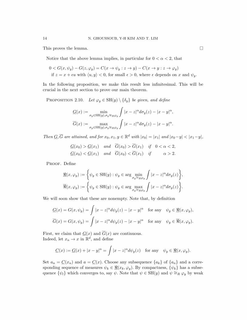
In the following proposition, we make this result less infinitesimal. This will becrucial in the next section to prove our main theorem.
Proposition 2.10. Let ϕy ∈ SH(y) \ δy be given, and define
G(x) := minσy∈SH(y),σy∼=Rϕy
∫|x− z|αdσy(z)− |x− y|α,
G(x) := maxσy∈SH(y),σy∼=Rϕy
∫|x− z|αdσy(z)− |x− y|α.
Then G,G are attained, and for x0, x1, y ∈ Rd with |x0| = |x1| and |x0−y| < |x1−y|,
G(x0) > G(x1) and G(x0) > G(x1) if 0 < α < 2,
G(x0) < G(x1) and G(x0) < G(x1) if α > 2.
Proof. Define
<(x, ϕy) :=
ψy ∈ SH(y) : ψy ∈ arg min
σy∼=Rϕy
∫|x− z|αdσy(z)
,
<(x, ϕy) :=
ψy ∈ SH(y) : ψy ∈ arg max
σy∼=Rϕy
∫|x− z|αdσy(z)
.
We will soon show that these are nonempty. Note that, by definition
G(x) = G(x, ψy) =
∫|x− z|αdψy(z)− |x− y|α for any ψy ∈ <(x, ϕy),
G(x) = G(x, ψy) =
∫|x− z|αdψy(z)− |x− y|α for any ψy ∈ <(x, ϕy).
First, we claim that G(x) and G(x) are continuous.Indeed, let xn → x in Rd, and define
C(x) := G(x) + |x− y|α =
∫|x− z|αdψy(z) for any ψy ∈ <(x, ϕy).
Set an = C(xn) and a = C(x). Choose any subsequence ak of an and a corre-sponding sequence of measures ψk ∈ <(xk, ϕy). By compactness, ψk has a subse-quence ψl which converges to, say ψ. Note that ψ ∈ SH(y) and ψ ∼=R ϕy by weak
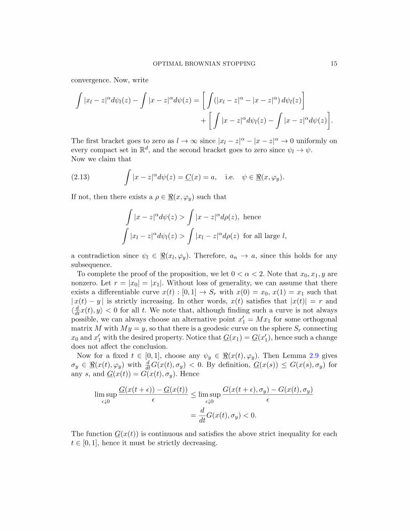
OPTIMAL BROWNIAN STOPPING 15
convergence. Now, write∫|xl − z|αdψl(z)−
∫|x− z|αdψ(z) =
[ ∫(|xl − z|α − |x− z|α) dψl(z)
]+
[ ∫|x− z|αdψl(z)−
∫|x− z|αdψ(z)
].
The first bracket goes to zero as l→∞ since |xl − z|α − |x− z|α → 0 uniformly onevery compact set in Rd, and the second bracket goes to zero since ψl → ψ.Now we claim that∫
|x− z|αdψ(z) = C(x) = a, i.e. ψ ∈ <(x, ϕy).(2.13)
If not, then there exists a ρ ∈ <(x, ϕy) such that∫|x− z|αdψ(z) >
∫|x− z|αdρ(z), hence∫
|xl − z|αdψl(z) >∫|xl − z|αdρ(z) for all large l,
a contradiction since ψl ∈ <(xl, ϕy). Therefore, an → a, since this holds for anysubsequence.
To complete the proof of the proposition, we let 0 < α < 2. Note that x0, x1, y arenonzero. Let r = |x0| = |x1|. Without loss of generality, we can assume that thereexists a differentiable curve x(t) : [0, 1] → Sr with x(0) = x0, x(1) = x1 such that|x(t) − y | is strictly increasing. In other words, x(t) satisfies that |x(t)| = r and〈 ddtx(t), y〉 < 0 for all t. We note that, although finding such a curve is not alwayspossible, we can always choose an alternative point x′1 = Mx1 for some orthogonalmatrix M with My = y, so that there is a geodesic curve on the sphere Sr connectingx0 and x′1 with the desired property. Notice that G(x1) = G(x′1), hence such a changedoes not affect the conclusion.
Now for a fixed t ∈ [0, 1], choose any ψy ∈ <(x(t), ϕy). Then Lemma 2.9 givesσy ∈ <(x(t), ϕy) with d
dtG(x(t), σy) < 0. By definition, G(x(s)) ≤ G(x(s), σy) forany s, and G(x(t)) = G(x(t), σy). Hence
lim supε↓0
G(x(t+ ε))−G(x(t))
ε≤ lim sup
ε↓0
G(x(t+ ε), σy)−G(x(t), σy)
ε
=d
dtG(x(t), σy) < 0.
The function G(x(t)) is continuous and satisfies the above strict inequality for eacht ∈ [0, 1], hence it must be strictly decreasing.
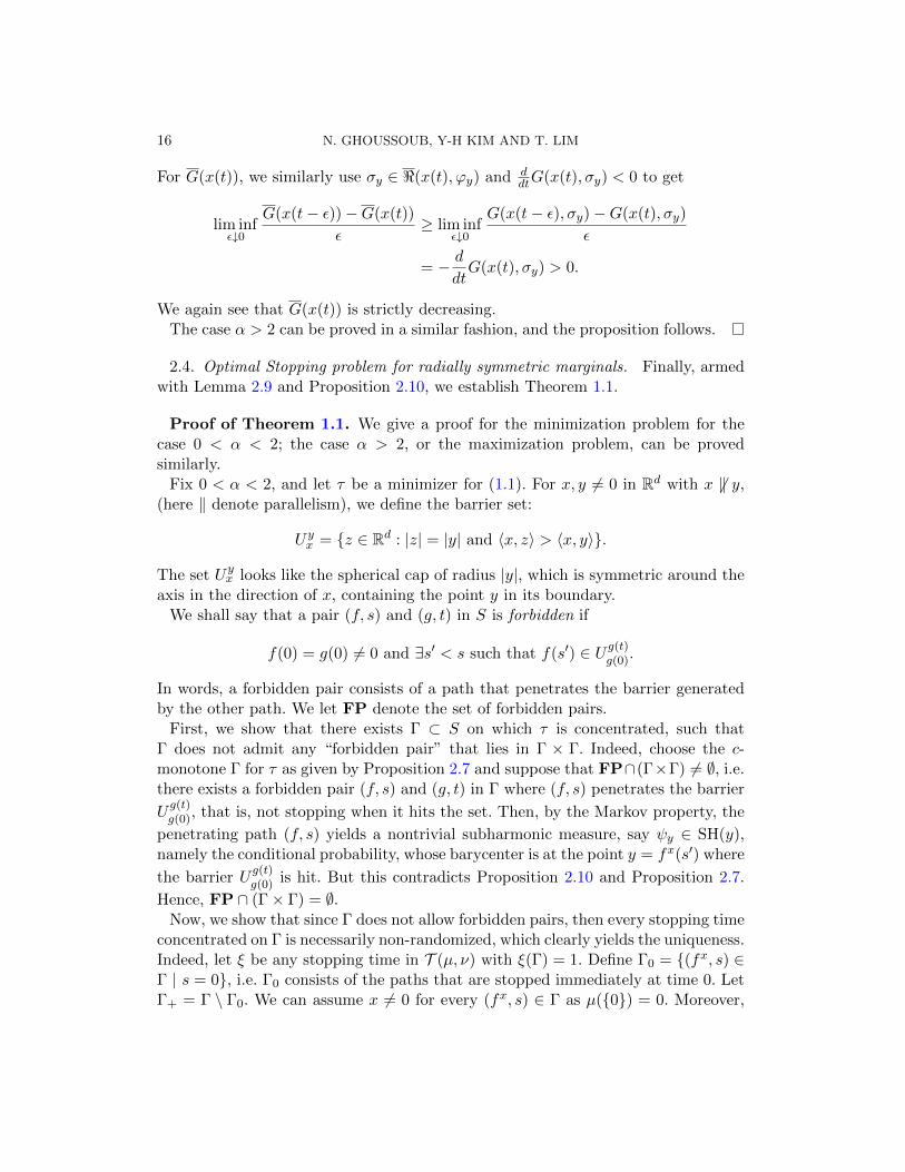
16 N. GHOUSSOUB, Y-H KIM AND T. LIM
For G(x(t)), we similarly use σy ∈ <(x(t), ϕy) and ddtG(x(t), σy) < 0 to get
lim infε↓0
G(x(t− ε))−G(x(t))
ε≥ lim inf
ε↓0
G(x(t− ε), σy)−G(x(t), σy)
ε
= − d
dtG(x(t), σy) > 0.
We again see that G(x(t)) is strictly decreasing.The case α > 2 can be proved in a similar fashion, and the proposition follows.
2.4. Optimal Stopping problem for radially symmetric marginals. Finally, armedwith Lemma 2.9 and Proposition 2.10, we establish Theorem 1.1.
Proof of Theorem 1.1. We give a proof for the minimization problem for thecase 0 < α < 2; the case α > 2, or the maximization problem, can be provedsimilarly.
Fix 0 < α < 2, and let τ be a minimizer for (1.1). For x, y 6= 0 in Rd with x 6‖ y,(here ‖ denote parallelism), we define the barrier set:
Uyx = z ∈ Rd : |z| = |y| and 〈x, z〉 > 〈x, y〉.
The set Uyx looks like the spherical cap of radius |y|, which is symmetric around theaxis in the direction of x, containing the point y in its boundary.
We shall say that a pair (f, s) and (g, t) in S is forbidden if
f(0) = g(0) 6= 0 and ∃s′ < s such that f(s′) ∈ Ug(t)g(0).
In words, a forbidden pair consists of a path that penetrates the barrier generatedby the other path. We let FP denote the set of forbidden pairs.
First, we show that there exists Γ ⊂ S on which τ is concentrated, such thatΓ does not admit any “forbidden pair” that lies in Γ × Γ. Indeed, choose the c-monotone Γ for τ as given by Proposition 2.7 and suppose that FP∩(Γ×Γ) 6= ∅, i.e.there exists a forbidden pair (f, s) and (g, t) in Γ where (f, s) penetrates the barrier
Ug(t)g(0), that is, not stopping when it hits the set. Then, by the Markov property, the
penetrating path (f, s) yields a nontrivial subharmonic measure, say ψy ∈ SH(y),namely the conditional probability, whose barycenter is at the point y = fx(s′) where
the barrier Ug(t)g(0) is hit. But this contradicts Proposition 2.10 and Proposition 2.7.
Hence, FP ∩ (Γ× Γ) = ∅.Now, we show that since Γ does not allow forbidden pairs, then every stopping time
concentrated on Γ is necessarily non-randomized, which clearly yields the uniqueness.Indeed, let ξ be any stopping time in T (µ, ν) with ξ(Γ) = 1. Define Γ0 = (fx, s) ∈Γ | s = 0, i.e. Γ0 consists of the paths that are stopped immediately at time 0. LetΓ+ = Γ \ Γ0. We can assume x 6= 0 for every (fx, s) ∈ Γ as µ(0) = 0. Moreover,
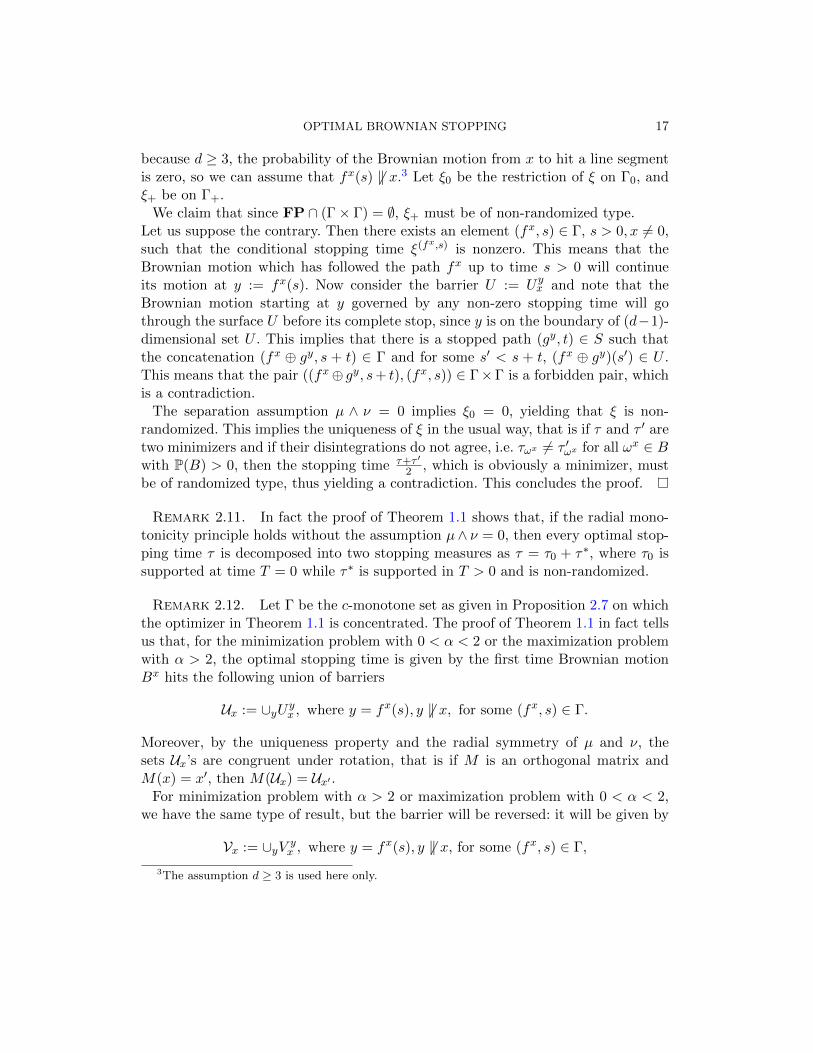
OPTIMAL BROWNIAN STOPPING 17
because d ≥ 3, the probability of the Brownian motion from x to hit a line segmentis zero, so we can assume that fx(s) 6‖ x.3 Let ξ0 be the restriction of ξ on Γ0, andξ+ be on Γ+.
We claim that since FP ∩ (Γ× Γ) = ∅, ξ+ must be of non-randomized type.Let us suppose the contrary. Then there exists an element (fx, s) ∈ Γ, s > 0, x 6= 0,such that the conditional stopping time ξ(fx,s) is nonzero. This means that theBrownian motion which has followed the path fx up to time s > 0 will continueits motion at y := fx(s). Now consider the barrier U := Uyx and note that theBrownian motion starting at y governed by any non-zero stopping time will gothrough the surface U before its complete stop, since y is on the boundary of (d−1)-dimensional set U . This implies that there is a stopped path (gy, t) ∈ S such thatthe concatenation (fx ⊕ gy, s + t) ∈ Γ and for some s′ < s + t, (fx ⊕ gy)(s′) ∈ U .This means that the pair ((fx⊕ gy, s+ t), (fx, s)) ∈ Γ×Γ is a forbidden pair, whichis a contradiction.
The separation assumption µ ∧ ν = 0 implies ξ0 = 0, yielding that ξ is non-randomized. This implies the uniqueness of ξ in the usual way, that is if τ and τ ′ aretwo minimizers and if their disintegrations do not agree, i.e. τωx 6= τ ′ωx for all ωx ∈ Bwith P(B) > 0, then the stopping time τ+τ ′
2 , which is obviously a minimizer, mustbe of randomized type, thus yielding a contradiction. This concludes the proof.
Remark 2.11. In fact the proof of Theorem 1.1 shows that, if the radial mono-tonicity principle holds without the assumption µ∧ ν = 0, then every optimal stop-ping time τ is decomposed into two stopping measures as τ = τ0 + τ∗, where τ0 issupported at time T = 0 while τ∗ is supported in T > 0 and is non-randomized.
Remark 2.12. Let Γ be the c-monotone set as given in Proposition 2.7 on whichthe optimizer in Theorem 1.1 is concentrated. The proof of Theorem 1.1 in fact tellsus that, for the minimization problem with 0 < α < 2 or the maximization problemwith α > 2, the optimal stopping time is given by the first time Brownian motionBx hits the following union of barriers
Ux := ∪yUyx , where y = fx(s), y 6‖ x, for some (fx, s) ∈ Γ.
Moreover, by the uniqueness property and the radial symmetry of µ and ν, thesets Ux’s are congruent under rotation, that is if M is an orthogonal matrix andM(x) = x′, then M(Ux) = Ux′ .
For minimization problem with α > 2 or maximization problem with 0 < α < 2,we have the same type of result, but the barrier will be reversed: it will be given by
Vx := ∪yV yx , where y = fx(s), y 6‖ x, for some (fx, s) ∈ Γ,
3The assumption d ≥ 3 is used here only.
18 N. GHOUSSOUB, Y-H KIM AND T. LIM
where V yx is the reversed barrier
V yx = z ∈ Rd : |z| = |y| and 〈x, z〉 < 〈x, y〉.
This is due to the interchange of the superharmonic and subharmonic region ofthe derivative of the gain function (2.11), according to the value of α. Also notethat when dealing with maximization problem, the inequalities (2.5) and (2.9) inthe monotonicity principles must be reversed.
Remark 2.13. Observe that in the above proof, the argument breaks down inthe two dimensional case, because the probability for a Brownian motion to hit aline segment is not zero when the dimension ≤ 2. Still, it shows that the optimal(possibly randomized) stopping time τ has to stop the Brownian path completelyonce it stops at a point not parallel to the initial point. Therefore, in particular, forthe minimization problem with 0 < α < 2, the set
Ux := ∪yUyx , where y = fx(s), y 6‖ x, for some (fx, s) ∈ Γ
is a barrier. However, there are chances that the Brownian path may stop onlypartially at points parallel to x, then to continue until it hits the set Ux. Similarresult holds for the maximization problem or with α > 2.
Finally, we note that the ideas in this section can be applied to costs that are moregeneral than the ones of the form |x−y|α considered in this paper. In particular, theyapply to a class of cost functions c(x, y) that are invariant under rotation and whosedirectional derivatives ∇uc(x, y) in the x-variable have suitable sub/superharmonicregions in the y-variable.
3. Subharmonic martingale optimal transport problem. In the previoussection we focused on the structure or optimal stopping times, utilizing the radialsymmetry of marginals. From now on we do not assume the radial symmetry butconsider general marginals. We assume compact support, but see Proposition 3.4 foran exception.
As mentioned in the introduction, a subharmonic function on an open subset of Rdmay not allow a subharmonic extension on all of Rd in general. When can f ∈ SH(O)be approximated by f ∈ SH(Rd) in O? To give an answer, we recall the following.
Lemma 3.1 (Walsh [43]). Let K be a compact subset of Rd such that Rd \K isconnected. Then for each ε > 0 and a harmonic function u on an open set containingK, there exists a harmonic polynomial v such that |u− v| < ε on K.
Keeping this in mind, we turn to the proof of Theorem 1.5. First we need thefollowing very likely known lemma. Given an open set O in Rd, let C(O) be the
OPTIMAL BROWNIAN STOPPING 19
space of continuous functions on O. We give a topology on C(O) which is inducedby the following convergence, namely, fn → f iff ||fn − f ||L∞(K) → 0 on everycompact subset K of O. It is clear that this topology is metrizable via the followingmetric
d(f, g) :=
∞∑n=1
2−n min(1, ||f − g||Kn)
where Kn is a compact exhaustion of O; Kn is compact, Kn ⊂ int(Kn+1), and∪nKn = O.
Lemma 3.2. The space H(O) of harmonic functions on O, is separable under d.
Proof. The space C(O) is separable under the metric d, e.g. the set Q[x1, ..., xd]of polynomials with rational coefficients is a countable dense subset of C(O) byStone-Weierstrass Theorem. Then since every subspace of a separable metric spaceis separable, H(O) is separable as well.
Proof of Theorem 1.5. To prove (1.8)), note that if π ∈ SMTRd(µ, ν), thenfor any p ∈ Ψ we have∫
p(x, y)dπ(x, y) =
∫p(x, y)dπx(y)dµ(x) ≥
∫p(x, x)dµ(x) = 0
in view of the subharmonicity of of y 7→ p(x, y). Hence we have the following inclu-sions
SMT(µ, ν) ⊂ SMTRd(µ, ν) ⊂π ∈ Π(µ, ν)
∣∣∣ ∫ p(x, y)dπ(x, y) ≥ 0 ∀p ∈ Ψ.
Now let π ∈ Π(µ, ν) and assume∫p dπ ≥ 0 for every p ∈ Ψ. We now prove that
π ∈ SMT(µ, ν). Indeed, let 1Bz,r be the indicator function on the ball Bz,r of centerz and radius r, and consider the functions of the form
p(x, y) = 1Bz,r(x)(ϕ(y)− ϕ(x)) where ϕ ∈ H(Rd).
Then p(x, y) ∈ Ψ4. For z ∈ suppµ, we have
0 ≤ 1
µ(Bz,r)
∫∫p(x, y)dπ(x, y) =
1
µ(Bz,r)
∫Bz,r
(∫ϕ(y)dπx(y)− ϕ(x)
)dµ(x)
→∫ϕ(y)dπz(y)− ϕ(z) as r → 0, µ− a.e. z,
4Technically 1Bz,r (x) is not continuous, but it can be approximated by continuous and compactlysupported functions.
20 N. GHOUSSOUB, Y-H KIM AND T. LIM
where the convergence is due to e.g. [33, Lemma 4.1.2.]. By changing ϕ 7→ −ϕ inp(x, y), we deduce ∫
ϕ(y)dπz(y) = ϕ(z) µ− a.e. z.(3.1)
One may notice that the µ - a.e. convergence set could depend on the choice of ϕ,but the application of Lemma 3.2 then ensures that the equality (3.1) holds for allϕ ∈ H(Rd), µ - a.e..
Let ψ be the fundamental solution of the Laplace equation, and let ψa(x) = ψ(x−a) and ψa,c(x) = max(ψ(x − a), c) where a ∈ Rd and c ∈ R. Note that ψa,c iscontinuous and subharmonic on Rd. By applying the above argument with p(x, y) =1Bz,r(x)(ψa,c(y)− ψa,c(x)) and letting c −∞, we deduce∫
ψa(y)dπz(y) ≥ ψa(z) for every a ∈ Rd, µ− a.e. z.(3.2)
Now let O be a regular domain for µ, ν, and let K be a compact set in O such thatsupp(µ+ ν) ⊂ K and Rd \K is connected. Let O′ be an open precompact subset ofO containing K. For each f ∈ SH(O), there exists a nonnegative Borel measure κon O such that f can be decomposed as
f(x) = h(x) +
∫O′ψa(x)dκ(a) ∀x ∈ O′, for some h ∈ H(O′)
by Riesz representation theorem. Let hε be a harmonic polynomial such that |h −hε| < ε on K by Walsh’s theorem. Then for µ-a.e. x, we have∫
f(y)dπx(y) =
∫h(y)dπx(y) +
∫Rd
∫O′ψa(y)dκ(a)dπx(y)
≥∫hε(y)dπx(y) +
∫O′
∫Rdψa(y)dπx(y)dκ(a)− ε
≥ hε(x) +
∫O′ψa(x)dκ(a)− ε
≥ h(x) +
∫O′ψa(x)dκ(a)− 2ε = f(x)− 2ε.
Letting ε → 0 we get∫f(y)dπx(y) ≥ f(x) µ-a.e. x, implying π ∈ SMTO(µ, ν). As
O ∈ R(µ, ν) was arbitrary we deduce that π ∈ SMT(µ, ν). This completes the proofof the equality (1.8).
Now we prove the equivalence in Theorem 1.5. Notice that (1) ⇐⇒ (2) is imme-diate by the same approximation argument as above. The direction (3) =⇒ (1) isalso immediate, as for f ∈ SH(Rd) and π ∈ SMT(µ, ν),∫
f(y)dν(y) =
∫f(y)dπx(y)dµ(x) ≥
∫f(x)dµ(x).
OPTIMAL BROWNIAN STOPPING 21
To see that (4) =⇒ (3), let O be an open ball containing supp(µ + ν), and takeτ ∈ TO(µ, ν). Then for f ∈ SH(Rd), since (f(Bt∧τ ))t is a submartingale, we have
E[f(Y ) | X] ≥ f(X), where X = B0 ∼ µ, Y = Bτ ∼ ν.
This means that the joint law of (X,Y ) belongs to SMT(µ, ν).It remains to show the implication (2) =⇒ (4). This will be done in Proposi-
tion 3.4 below, where we prove it for possibly non-compactly supported marginals.Finally, let now π ∈ SMT(µ, ν) and its disintegration (πx)x with respect to µ. Let
(Bt)t be a Brownian motion with B0 ∼ µ, and let O ∈ R(µ, ν) be bounded. Sinceδx ≺s(O) πx for µ-almost all x, and noting that B0 and Bt−B0 are independent, onecan apply the implication (2)⇒ (4) to the subharmonic ordered pair (δx, πx), and usethe measurable selection theorem, to find a stopping time τ = τ ∧τO such that givenB0, we have Law(Bτ ∈ · |B0) = πB0( · ). It is then clear that Law(B0, Bτ ) = π.
The following is now immediate.
Corollary 3.3. Let µ, ν ∈ Pc(Rd) and assume µ ≺s ν. Then
inf E [c(B0, Bτ )] | τ ∈ T (µ, ν) = inf
∫∫c(x, y)dπ |π ∈ SMT(µ, ν)
.
The following proposition may have its own interest. Let P2(O) be the set ofprobability measures concentrated in O and with finite second moments. Define theorder µ ≺s2(O) ν by
µ ≺s2(O) ν ⇐⇒∫fdµ ≤
∫fdν for every f ∈ SH(O) with f(x) ≤ Cf (1 + |x|2).
Proposition 3.4. Let µ, ν ∈ P2(O) and assume µ ≺s2(O) ν. Then TO(µ, ν) 6= ∅.
Remark 3.5. For the proposition, we need not assume O is regular since theproof clearly implies that if µ, ν ∈ Pc(O) are such that µ ≺s(O) ν, then necessarilyTO(µ, ν) 6= ∅.
To prove the proposition, we first introduce the notion of spherical martingales.
Definition 3.6. Let U be the uniform probability measure on the unit sphereSd−1 in Rd. Let (Xi)
∞i=1 be i.i.d random variables on some probability space (Ω,P),
whose distribution is U . A stochastic process (Fn)n≥0 is called a spherical martingale(valued) in O if there is an associated sequence of bounded measurable functions
rn : Rd × Sd−1 × · · · × Sd−1︸ ︷︷ ︸(n−1)−times
→ R+
22 N. GHOUSSOUB, Y-H KIM AND T. LIM
such that
Fn(X1, ..., Xn)− Fn−1(X1, ..., Xn−1) = rn(F0, X1, ..., Xn−1) ·Xn
and if for every n ∈ N, 0 ≤ λ ≤ 1 and (X1, X2, ..., Xn),
Fn−1(X1, ..., Xn−1) + λrn(F0, X1, ..., Xn−1)Xn ∈ O.
At each time n, a particle splits uniformly onto a surrounding sphere of radiusrn. An important observation is that the push-forward measure of δx by a sphericalmartingale Fn has the same law as Bx
τ , where the stopping time τ is defined asfollows: τ1 is the first time Bx hits the sphere S(x, r1(x)) centered at x and withradius r1(x). If Bτ1(ω) = x1 ∈ S(x, r1(x)), then define τ2 to be the first hitting timeBx1 hits the sphere S(x1, r2(x, x1)). One can then define inductively a sequence ofstopping times τ1 ≤ τ2 ≤ ... such that Fn(P) = Law(Bx
τn).The following lemma is an analogue of a result of Bu-Schachermayer [8, Proposition
2.1] about analytic martingales.
Lemma 3.7. Let O be an open set in Rd and f : O → R ∪ −∞ be an uppersemicontinuous function. Then there exists a unique maximal subharmonic functionf on O which is dominated by f . In other words, f ≤ f and g ≤ f for everyg ∈ SH(O) with g ≤ f . Furthermore, f can be constructed as follows:For each n ∈ N, define fn on O by
fn(x) = infE[f(Fn)] : (Fi)ni=0 is a spherical martingale in O with F0 = x(3.3)
and Fn(P) is compactly supported in O.
Then, the sequence (fn)∞n=0 decreases pointwise to f .
Proof. We will use an equivalent form of (3.3):
f0 = f and for n ≥ 1, fn(x) = inf
∫fn−1(x+ ry) dU(y)
where the infimum is taken over all r ≥ 0 such that x+ rB ⊂ O. Here, x+ rBdenotes the closed ball of radius r around x.
First note that the sequence (fn)∞n=0 is decreasing. To show the upper-semicontinuityof f , we proceed inductively and assume fn−1 is upper semicontinuous. If (xk)
∞k=0
in O is such that limk→∞ xk = x0, and r ≥ 0 is such that x0 + rB ⊂ O, where Bis the closed unit ball, then there is k0 such that xk + rB ⊂ O for k ≥ k0. Theupper semicontinuous function fn−1 is bounded above on the relatively compact set∪∞k=k0
xk + rB and, for every z ∈ B, fn−1(x0 + rz) ≥ lim supk→∞ fn−1(xk + rz).Hence by Fatou’s lemma,∫
fn−1(x0 + ry) dU(y) ≥ lim supk→∞
∫fn−1(xk + ry) dU(y) ≥ lim sup
k→∞fn(xk).
OPTIMAL BROWNIAN STOPPING 23
Thus fn(x0) ≥ lim supk→∞
fn(xk), hence showing that fn and consequently f is upper-
semicontinuous.Let now g be a subharmonic function on O with g ≤ f . Again, inductively, assum-
ing that g ≤ fn−1, then for x0 + rB ⊂ O,∫fn−1(x0 + ry) dU(y) ≥
∫g(x0 + ry) dU(y) ≥ g(x0),
and so fn(x0) ≥ g(x0). Hence f ≥ g. Finally, for x0 + rB ⊂ O, we get frommonotone convergence
f(x0) = limn→∞
fn(x0) ≤ limn→∞
∫fn−1(x0 + ry) dU(y) =
∫f(x0 + ry) dU(y).
This shows that f is subharmonic, and the proof of the lemma is complete.
Let now Lip∗(O) be the space of all finite measures in O with finite first moments.
Lemma 3.8. Let µ, ν ∈ P2(O) be such that µ ≺s2(O) ν, and consider the followingsubset of P2(O),
Φ = Fn(P) : (Fi)ni=0 is a spherical martingale valued in O with F0 ∼ µ.
Set ν := (1 + |x|)ν and
Φ = (1 + |x|)Φ := σ | σ = (1 + |x|)σ for some σ ∈ Φ.
Then, ν is in the weak∗-closure of Φ in Lip∗(O).
Proof. Observe first that Φ is convex. Indeed, if (F ′i )ni=0 and (F ′′i )mi=0 are two
spherical martingales with F ′0 ∼ µ, F ′′0 ∼ µ, we may assume n = m, then define aspherical martingale (Fi)
n+1i=0 by letting F0 = F1 ∼ µ and for 1 ≤ i ≤ n,
Fi+1(X1, X2, ..., Xi+1) =
F ′i (X2, ..., Xi+1) if X1 is in the upper hemisphere,
F ′′i (X2, ..., Xi+1) if X1 is in the lower hemisphere.
Clearly Fn+1(P) = F ′n(P) + F ′′n (P)/2 and hence Φ is convex, and therefore Φ =(1 + |x|)Φ is convex in Lip∗(O).
If now the statement of the lemma were false, then by the Hahn-Banach theoremwe can find a Lipschitz function f on O and real numbers a < b such that∫
g dν ≤ a, while
∫g Fn dP ≥ b for every Fn(P) ∈ Φ,
where g(x) = (1 + |x|)f(x). But since every element in Φ has initial distributionµ, then by Lemma 3.7 and (3.3), we have
∫g dµ ≥ b and therefore a ≥
∫g dν ≥∫
g dν ≥∫g dµ ≥ b, which is a contradiction.
24 N. GHOUSSOUB, Y-H KIM AND T. LIM
Proof of Proposition 3.4. By Lemma 3.8, we have a sequence νn ⊂ Φ suchthat
∫|x|2dνn(x) →
∫|x|2dν(x). We know that νn = Law(Bτn) for a sequence of
stopping times τn and a Brownian motion B with initial law µ. Hence in particularEτn = E|Bτn |2 =
∫|x|2dνn(x) ≤ V for some constant V and for all n. The sequence
(τn) is then tight, and it is standard that it has a convergent subsequence to a –possibly randomized– stopping time τ in such a way that Ef(Bτk) → Ef(Bτ ) forevery f continuous and bounded function on Rd. (see for example [1] or [2]). In otherwords, Law(Bτk)→ Law(Bτ ), and therefore, Bτ ∼ ν. Let τO be the first exit time of(Bt) from O and note that τk = τk ∧ τO by the definition of Φ, and therefore τ alsosatisfies τ = τ ∧ τO. Notice also that Eτ = E|Bτ |2 ≤ V as well, hence the martingale(Bτ∧t)t≥0 is bounded in L2.
Lastly, we prove the duality result announced in the introduction.
Proof of Theorem 1.6. By a standard argument, it is enough to prove the theo-rem for continuous cost c, so let us assume this. Clearly, the left-hand side is smallerthan or equal to the right-hand side since for every π ∈ SMT(µ, ν) (if exists) andfor every (α, β, p) ∈ Kc, we have
∫p(x, y)dπ(x, y) ≥ 0.
For the reverse inequality, we first note that Kantorovich duality for the standardoptimal transport problem with a continuous cost c(x, y)− p(x, y) yields
sup(α,β,p)∈Kc
(∫βdν −
∫αdµ
)= sup
p∈Ψinf
π∈Π(µ,ν)
∫(c− p)dπ.
Now it is standard to apply a min-max theorem (see e.g. [3, Theorem 2]) to inter-change the order of inf and sup, and thereby obtain
sup(α,β,p)∈Kc
(∫βdν −
∫αdµ
)= inf
π∈Π(µ,ν)supp∈Ψ
∫(c− p)dπ.(3.4)
Note that the supremum over p can be finite only when∫p(x, y)dπ(x, y) ≥ 0, since
otherwise we can replace p with λp for some λ > 0, making the value of the integral∫(c−p)dπ arbitrarily large. Therefore, by Theorem 1.5, the infimum in (3.4) can be
restricted to π ∈ SMT(µ, ν), and we obtain
sup(α,β,p)∈Kc
(∫βdν −
∫αdµ
)= inf
π∈SMT(µ,ν)supp∈Ψ
∫(c− p)dπ.
Finally, since 0 ∈ Ψ, the last expression is greater than or equal to
inf
∫c(x, y)dπ | π ∈ SMT(µ, ν)
.
Together with Corollary 3.3, this completes the proof of the duality for the subhar-monic martingale optimal transport problem.
OPTIMAL BROWNIAN STOPPING 25
4. Appendix: The radially symmetric monotonicity principle. In thissection we use the dual attainment result [23] to provide a proof of Proposition 2.7.
Proof of Proposition 2.7. Let O be an open ball containing supp(µ+ν). First,we can assume without loss of generality that suppµ ∩ supp ν = ∅. Indeed, dueto the assumption µ ∧ ν = 0 and µ(∂ suppµ) = 0, for each µ-a.e. x, x′, we canconsider the restriction of µ to µ+ on an open set containing x, x′ outside supp νand let ν+ be the corresponding target measure under the stopping time τ . Thensuppµ+ ∩ supp ν+ = ∅. It will be sufficient to prove the desired conclusion of theproposition for those x, x′ ∈ suppµ+, suppϕy ⊂ supp ν+, and y′ ∈ supp ν+.
Now, from [23, Theorem 4.1 and the proof of Theorem 7.1 (1)] we have the existenceof the optimizers for the dual problem. Here, note that the theorems in [23] can beused because suppµ ∩ supp ν = ∅, the function c(x, y) = ±|x − y|α, α > 0, is C2
for those x, y ∈ suppµ× supp ν; this cost can be modified by adding an appropriatesubharmonic function h(y), with large ∆h, to an equivalent cost y 7→ c(x, y) + h(y)with 0 ≤ ∆y[c(x, y) + h(y)] which is C2 on suppµ× supp ν. Then, as in the proof of[23, Theorem 7.1 (1)] this can be extended to a C2 subharnonic function on O ×Owithout changing the optimal solution. The result [23, Theorem 4.1] can be appliedto this cost to get the dual optimizers, first β ∈ H1
0 (O) ∩ LSC(O), then
J(x, y) := supξ≤τO
[β(Byξ )− c(x,By
ξ )],(4.1)
where ξ is a stopping time for Brownian motion, and τO is the exit time from thedomain O. Set α(x) = J(x, x) and p(x, y) = J(x, x)− J(x, y).
From the radial symmetry of µ and ν, and the expression of the dual problem,we can assume that the dual optimizer β is radially symmetric. To see this, recallthat M is the group of d× d orthogonal matrices and H is the Haar measure on M.Then, for each M ∈M,
J(Mx,My) = α(Mx)− p(Mx,My) = supMξ≤τO
[β(BMy
Mξ )− c(Mx,BMyMξ )
].
Since both Brownian motion and the cost c(x, y) = ±|x − y|α are invariant underthe orthogoal group (isometries of Rd) we see that for
J(x, y) =
∫M∈M
J(Mx,My)dH(M) and β(y) =
∫M∈M
β(My)dH(M),
it holds that
J(x, y) = supξ≤τO
[β(By
ξ )− c(x,Byξ )].
Notice that β, α(x) := J(x, x) and p(x, y) := J(x, x)−J(x, y) are admissible and theyhave the same optimal dual value as
∫βdν −
∫αdµ, thus they are dual optimizers.
26 N. GHOUSSOUB, Y-H KIM AND T. LIM
The rest of the proof is similar to that of [23, Theorem B.1]. We will use the radialsymmetry of β. We notice that the desired conclusion of our theorem is equivalentto the following:
Claim 4.1. Let π be the measure with (B0, Bτ ) ∼ π. Consider a randomizedstopping time ξ with B0 ∼ µ, (B0, Bξ) ∼ σ where the disintegration σ(dx, dy) =σx(dy)µ(dx) satisfies
(4.2) 0 ≺s(O) σx ≺s(O) πx for each µ-a.e. x,
which means that σ ≤ τ , and τ − σ is a (randomized) stopping time.Then, for π-a.e. (x′, y′) and σ-a.e. (x, y), it holds that if |y| = |y′|, then the stopping
time τ − ξ restricted to paths with Bξ = y satisfies
c(x′, y′) + E[c(x,By
τ−ξ)]≤ E
[c(x′, By′
τ ′ )]
+ c(x, y),
for any stopping time τ ′ such that By′
τ ′ ∼ ϕy′ ∼=R ψy ∼ Byτ−ξ.
To prove this claim notice that from [23, Theorem 4.7], we have for π∗-a.e. (x′, y′)and σ-a.e. (x, y),
J(x′, y′) = β(y′)− c(x′, y′),(4.3)
J(x,Byτ−ξ) = J(x,Bx
τ ) = β(Bxτ )− c(x,Bx
τ ) = β(Byτ−ξ)− c(x,B
yτ−ξ).(4.4)
On the other hand, from the definition (4.1), we have
J(x′, y′) ≥ E[β(By′
τ ′ )− c(x′, By′
τ ′ )]
= E[β(By
τ−ξ)− c(x′, By′
τ ′ )]
(4.5)
where the first inequality holds for any τ ′ and the second one holds in particular for
those with By′
τ ′ ∼ ϕy′ ≡R ψy ∼ Byτ−ξ due to radial symmetry of β. Notice that from
[23, Theorem 4.7 (4.4)] we have
E[J(x,By
τ−ξ)]
= J(x, y).(4.6)
Moreover,
J(x, y) ≥ β(y)− c(x, y) = β(y′)− c(x, y)
where the last equality uses the radial symmetry of β and the fact that |y| = |y′|.Taking the expectation in (4.4), we see that the left hand sides of (4.3), (4.4) are
equal to the left hand sides of inequalities (4.5) and (4.6). Now, subtract the sum ofthe two equations from the sum of the two inequalities and cancel the terms β(y)and E
[β(By
τ−ξ)], to obtain
0 ≥ −c(x, y)− E[c(x′, By′
τ ′ )]
+ c(x′, y′) + E[c(x,By
τ−ξ)],
hence completing the proof.
OPTIMAL BROWNIAN STOPPING 27
REFERENCES
[1] J. R. Baxter and R. V. Chacon, Potentials of stopped distributions. Illinois J. Math., 18:649–656, (1974).
[2] M. Beiglbock, A.M.G. Cox, and M. Huesmann, Optimal transport and Skorokhod embedding.Inventiones mathematicae, Volume 208, Issue 2 (2017) 327–400.
[3] M. Beiglbock, P. Henry-Labordere, and F. Penkner, Model-independent bounds for optionprices–a mass transport approach. Finance and Stochastics, Volume 17 (2013) 477–501.
[4] M. Beiglbock, P. Henry-Labordere, and N. Touzi, Monotone martingale transport plans andSkorohod Embedding. Stochastic Processes and their Applications, Volume 127, Issue 9 (2017)3005–3013.
[5] M. Beiglbock and N. Juillet, On a problem of optimal transport under marginal martingaleconstraints. Ann. Probab, Volume 44 (2016) 42–106.
[6] M. Beiglbock, M. Nutz, and N. Touzi, Complete duality for martingale optimal transport onthe line. Ann. Probab., Volume 45, Number 5 (2017) 3038–3074.
[7] Y. Brenier, Polar factorization and monotone rearrangement of vector-valued functions. Com-munications on pure and applied mathematics, Volume 44, Issue 4 (1991) 375–417.
[8] S. Bu and W. Schachermayer, Approximation of Jensen measures by image measures underholomorphic functions and applications. Trans. Amer. Math. Soc., Volume 331 (1992) 585–608.
[9] R. V. Chacon and J. B. Walsh, One-dimensional potential embedding. In Seminaire deProbabilites, X. Lecture Notes in Math., Vol. 511. Springer, Berlin (1976), 19–23. MR445598.
[10] G. Choquet, Forme abstraite du theoreme de capacitabilite. Ann. Inst. Fourier. Grenoble,Volume 9 (1959) 83–89.
[11] A.M.G. Cox, J. Ob loj, and N. Touzi, The Root solution to the multi-marginal embeddingproblem: an optimal stopping and time-reversal approach. Probability Theory and RelatedFields (Open Access), (2018).
[12] H. De March and N. Touzi, Irreducible convex paving for decomposition of multi-dimensionalmartingale transport plans. https://arxiv.org/abs/1702.08298 (2017).
[13] Y. Dolinsky and H.M. Soner, Martingale optimal transport and robust hedging in continuoustime. Probab. Theory Relat. Fields, 160 (2014) 391–427.
[14] Y. Dolinsky and H.M. Soner, Martingale optimal transport in the Skorokhod space. StochasticProcesses and their Applications, 125(10) (2015) 3893–3931.
[15] G.A. Edgar, Complex martingale convergence. Banach Spaces, Volume 1166 of the seriesLecture Notes in Mathematics, 38–59.
[16] G.A. Edgar, Analytic martingale convergence. Journal of Functional Analysis, Volume 69,Issue 2, November 1986, 268–280.
[17] N. Falkner, On Skorohod embedding in n-dimensional Brownian motion by means of naturalstopping times. In Seminaire de Probabilites, XIV, volume 784 of Lecture Notes in Math.,357–391. Springer, Berlin, (1980). MR580142.
[18] G.B. Folland. Real analysis: modern techniques and their applications. John Wiley & Sons,2013.
[19] A. Galichon, P. Henry-Labordere, and N. Touzi, A Stochastic Control Approach to No-Arbitrage Bounds Given Marginals, with an Application to Lookback Options. Ann. Appl.Probab, Volume 24, Number 1 (2014) 312–336.
[20] W. Gangbo and R.J. McCann, The geometry of optimal transportation. Acta Math, Volume177, Issue 2 (1996) 113–161.
[21] N. Ghoussoub, Y-H. Kim, and T. Lim, Structure of optimal martingale transport in generaldimensions. Annals of Probability, Vol. 47, No. 1, (2019) 109-164
28 N. GHOUSSOUB, Y-H KIM AND T. LIM
[22] N. Ghoussoub, Y-H. Kim, and T. Lim, Optimal Skorokhod Embedding for radially symmetricmarginals arXiv:1711.02784
[23] N. Ghoussoub, Y.-H. Kim, and A.Z. Palmer. A solution to the Monge transport problem forBrownian martingales. arXiv:1903.00527
[24] N. Ghoussoub, Y.-H. Kim, and A.Z. Palmer, PDE Methods for Optimal Skorokhod Embed-dings, Calculus of Variations and PDE, 58: 113.: 1-33.
[25] N. Ghoussoub and B. Maurey, Plurisubharmonic martingales and barriers in complex quasi-Banach spaces. Annales de l’institut Fourier, Volume 39, Issue 4 (1989) 1007–1060.
[26] G. Guo, X. Tan, and N. Touzi, Optimal Skorokhod embedding under finitely-many marginalconstraints. SIAM J. Control Optim, 54(4), (2016) 2174–2201.
[27] D. Hobson, Robust hedging of the lookback option, Finance and Stochastics, 2 (1998) 329–347.
[28] D. Hobson, The Skorokhod embedding problem and model-independent bounds for optionprices. In Paris-Princeton Lectures on Mathematical Finance 2010, volume 2003 of LectureNotes in Math, Springer, Berlin (2011) 267–318.
[29] D. Hobson and M. Klimmek, Robust price bounds for the forward starting straddle. Financeand Stochastics, Volume 19, Issue 1 (2014) 189–214.
[30] D. Hobson and A. Neuberger, Robust bounds for forward start options. Mathematical Finance,Volume 22, Issue 1 (2012) 31–56.
[31] J. A. Johnson, Banach spaces of Lipschitz functions and vector-valued Lipschitz functions.Bull. Amer. Math. Soc, Volume 75, Number 6 (1969), 1334–1338.
[32] S. Kallblad, X. Tan and N. Touzi, Optimal Skorokhod embedding given full marginals andAzema-Yor peacocks. Ann. Appl. Probab, Volume 27, Number 2 (2017), 686–719.
[33] F. Ledrappier and L.-S. Young, The Metric Entropy of Diffeomorphisms: Part I: Characteriza-tion of Measures Satisfying Pesin’s Entropy Formula. Annals of Mathematics, Second Series,Vol. 122, No. 3 (1985), 509–539.
[34] T. Lim, Optimal martingale transport between radially symmetric marginals in general di-mensions. https://arxiv.org/abs/1412.3530, (2016).
[35] I. Monroe, On embedding right continuous martingales in Brownian motion. The Annals ofMathematical Statistics, Vol. 43, No. 4, 1293–1311 (1972).
[36] J. Ob loj, The Skorokhod embedding problem and its offspring Probability Surveys, 1 (2004)321–392.
[37] J. Ob loj and P. Siorpaes, Structure of martingale transports in finite dimensions.https://arxiv.org/abs/1702.08433 (2017).
[38] J. Ob loj and P. Spoida, An Iterated Azema-Yor Type Embedding for Finitely Many Marginals.Ann. Probab., to appear. (2016)
[39] H. Rost, The Stopping Distributions of a Markov Process. Inventiones mathematicae, 14, 1–16(1971).
[40] A.V. Skorokhod, Studies in the Theory of Random Processes (Translated from the Russian byScripta Technica Inc.). Addison-Wesley Publishing Co. Inc., Reading (1965)
[41] V. Strassen, The existence of probability measures with given marginals. Ann. Math. Statist.,36 (1965) 423–439.
[42] C. Villani, Topics in optimal transportation, Volume 58, Graduate Studies in Mathematics.American Mathematical Society, Providence, RI, 2003.
[43] J.L. Walsh, The approximation of harmonic functions by harmonic polynomials and by har-monic rational functions. Bull. Amer. Math. Soc. (2) 35 (1929) 499–544.

OPTIMAL BROWNIAN STOPPING 29
Department of MathematicsUniversity of British ColumbiaVancouver, V6T 1Z2 CanadaE-mail: [email protected]
Institute of Mathematical SciencesShanghaiTech UniversityNo. 393, Huaxia Middle Road, Pudong New Area, Shanghai 201210E-mail: [email protected]