Optical Properties with Wien2k - Pennsylvania State … Properties with Wien2k ... free e : Lindhard...
35
Optical Properties with Wien2k Elias Assmann Vienna University of Technology, Institute for Solid State Physics WIEN2013@PSU, Aug 13
Transcript of Optical Properties with Wien2k - Pennsylvania State … Properties with Wien2k ... free e : Lindhard...
Optical Properties with Wien2k
Elias Assmann
Vienna University of Technology,Institute for Solid State Physics
WIEN2013@PSU, Aug 13
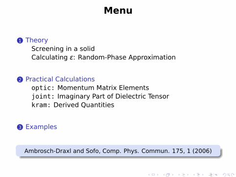
Menu
1 TheoryScreening in a solidCalculating ϵ: Random-Phase Approximation
2 Practical Calculationsoptic: Momentum Matrix Elementsjoint: Imaginary Part of Dielectric Tensorkram: Derived Quantities
3 Examples
Ambrosch-Draxl and Sofo, Comp. Phys. Commun. 175, 1 (2006)
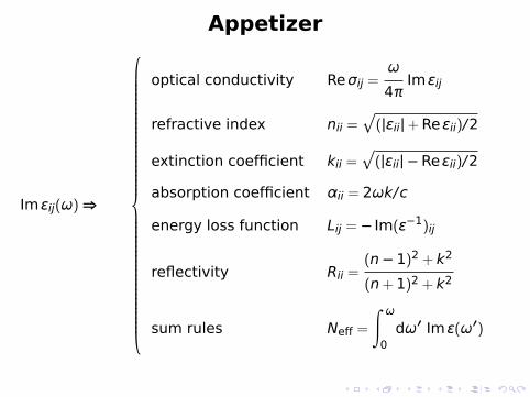
Appetizer
Im ϵij(ω)⇒
optical conductivity Reσij =ω
4πIm ϵij
refractive index nii =p
(|ϵii|+Re ϵii)/2
extinction coefficient kii =p
(|ϵii| −Re ϵii)/2
absorption coefficient αii = 2ωk/c
energy loss function Lij = − Im(ϵ−1)ij
reflectivity Rii =(n− 1)2 + k2
(n+ 1)2 + k2
sum rules Neff =
∫ ω
0dω′ Im ϵ(ω′)
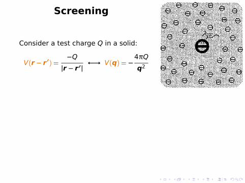
Screening
Consider a test charge Q in a solid:
V(r − r′) =−Q|r − r′|
←→ V(q) = −4πQ
q2
e− will move to screen the charge effective potential W;
dielectric function “V = ϵW”
Simplest model: Thomas-Fermi
W(r) =e−kTFr
r←→ W(q) =
4π
kTF2 +q2
k2TF = 4πN (EF)
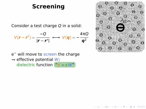
Screening
Consider a test charge Q in a solid:
V(r − r′) =−Q|r − r′|
←→ V(q) = −4πQ
q2
e− will move to screen the charge effective potential W;
dielectric function “V = ϵW”
Simplest model: Thomas-Fermi
W(r) =e−kTFr
r←→ W(q) =
4π
kTF2 +q2
k2TF = 4πN (EF)
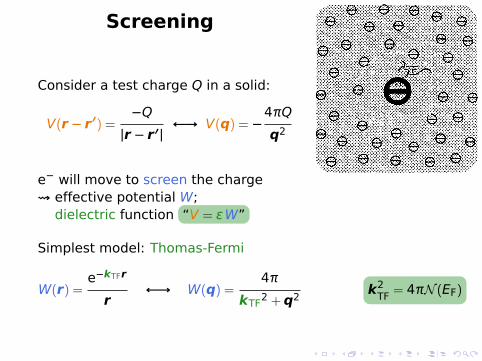
Screening
Consider a test charge Q in a solid:
V(r − r′) =−Q|r − r′|
←→ V(q) = −4πQ
q2
e− will move to screen the charge effective potential W;
dielectric function “V = ϵW”
Simplest model: Thomas-Fermi
W(r) =e−kTFr
r←→ W(q) =
4π
kTF2 +q2
k2TF = 4πN (EF)
Ansatz for W
R
d d′
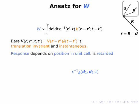
r = R+d
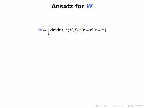
W ∼∫
dr′dt ϵ−1(r′; t)V(r − r′; t − t′)
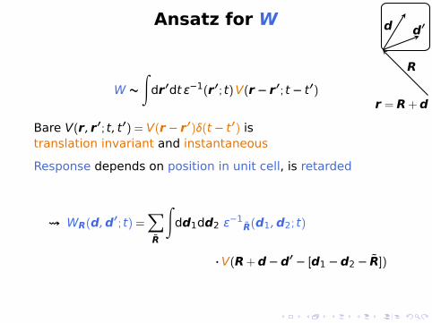
Bare V(r, r′; t, t′) = V(r − r′)δ(t − t′) istranslation invariant and instantaneous
Response depends on position in unit cell, is retarded
WR(d,d′; t) =∑
R
∫
dd1dd2
ϵ−1R(d1,d2; t)
· V(R+d−d′ − [d1 −d2 − R])
Ansatz for W
R
d d′
r = R+dW ∼∫
dr′dt ϵ−1(r′; t)V(r − r′; t − t′)
Bare V(r, r′; t, t′) = V(r − r′)δ(t − t′) istranslation invariant and instantaneous
Response depends on position in unit cell, is retarded
WR(d,d′; t) =∑
R
∫
dd1dd2
ϵ−1R(d1,d2; t)
· V(R+d−d′ − [d1 −d2 − R])
Ansatz for W
R
d d′
r = R+dW ∼∫
dr′dt ϵ−1(r′; t)V(r − r′; t − t′)
Bare V(r, r′; t, t′) = V(r − r′)δ(t − t′) istranslation invariant and instantaneous
Response depends on position in unit cell, is retarded
WR(d,d′; t) =∑
R
∫
dd1dd2 ϵ−1R(d1,d2; t)
· V(R+d−d′ − [d1 −d2 − R])
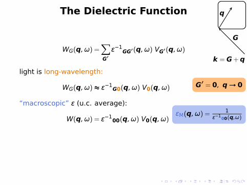
The Dielectric Function
G
q
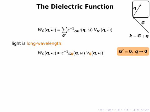
k =G+q
WG(q, ω) =∑
G′ϵ−1
GG′(q, ω) VG′(q, ω)
light is long-wavelength:
G′ = 0, q→ 0WG(q, ω) ≈ ϵ−1G0(q, ω) V0(q, ω)
“macroscopic” ϵ (u.c. average):ϵM(q, ω) = 1
ϵ−100(q,ω)W(q, ω) = ϵ−100(q, ω) V0(q, ω)
neglect local-field effects:
ϵM(q, ω) ≈ ϵ00(q, ω)
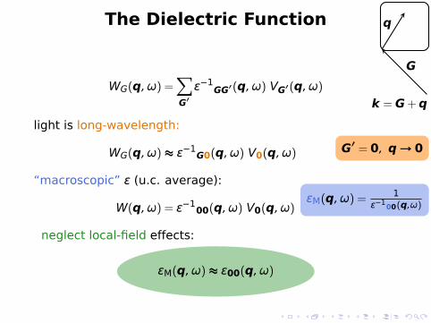
The Dielectric Function
G
q
k =G+q
WG(q, ω) =∑
G′ϵ−1
GG′(q, ω) VG′(q, ω)
light is long-wavelength:
G′ = 0, q→ 0WG(q, ω) ≈ ϵ−1G0(q, ω) V0(q, ω)
“macroscopic” ϵ (u.c. average):ϵM(q, ω) = 1
ϵ−100(q,ω)W(q, ω) = ϵ−100(q, ω) V0(q, ω)
neglect local-field effects:
ϵM(q, ω) ≈ ϵ00(q, ω)
The Dielectric Function
G
q
k =G+q
WG(q, ω) =∑
G′ϵ−1
GG′(q, ω) VG′(q, ω)
light is long-wavelength:
G′ = 0, q→ 0WG(q, ω) ≈ ϵ−1G0(q, ω) V0(q, ω)
“macroscopic” ϵ (u.c. average):ϵM(q, ω) = 1
ϵ−100(q,ω)W(q, ω) = ϵ−100(q, ω) V0(q, ω)
neglect local-field effects:
ϵM(q, ω) ≈ ϵ00(q, ω)
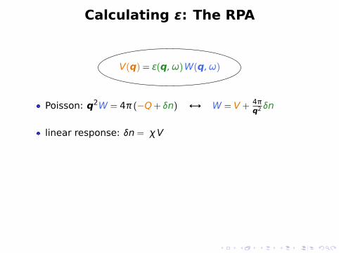
Calculating ϵ: The RPA
V(q) = ϵ(q, ω)W(q, ω)
Poisson: q2W = 4π (−Q+ δn) ↔ W = V + 4πq2 δn
linear response: δn = χV
PW → V = (1− 4πq2 P)W
“random-phase” approximation: P to lowest order
P = + + + · · ·
∼ G0(1,2)G0(2,1)
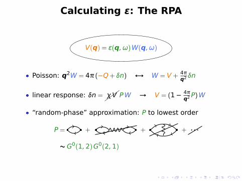
Calculating ϵ: The RPA
V(q) = ϵ(q, ω)W(q, ω)
Poisson: q2W = 4π (−Q+ δn) ↔ W = V + 4πq2 δn
linear response: δn = χV PW → V = (1− 4πq2 P)W
“random-phase” approximation: P to lowest order
P = + + + · · ·
∼ G0(1,2)G0(2,1)
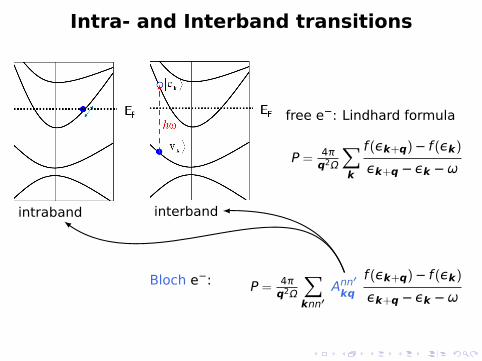
Intra- and Interband transitions
intraband interband
free e−: Lindhard formula
P = 4πq2Ω
∑
k
f (εk+q)− f (εk)εk+q − εk −ω
Bloch e−: P = 4πq2Ω
∑
knn′Ann
′
kq
f (εk+q)− f (εk)εk+q − εk −ω
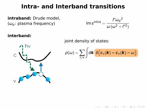
Intra- and Interband transitions
intraband: Drude model,(ωp: plasma frequency) Im ϵintra =
ωp2
ω (ω2 + 2)
interband:joint density of states:
ρ(ω) =∑
c,v
∫
dk δ
εc(k)− εv(k)−ω
v-c transition probability(“selection rules”) given bymomentum matrix elements
Im ϵij(ω,0) ∝1ω2
∑
c,v
∫
dk δ
εc(k)− εv(k)−ω
⟨ck|bpi|vk⟩ ⟨vk|bpj|ck⟩
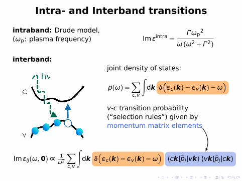
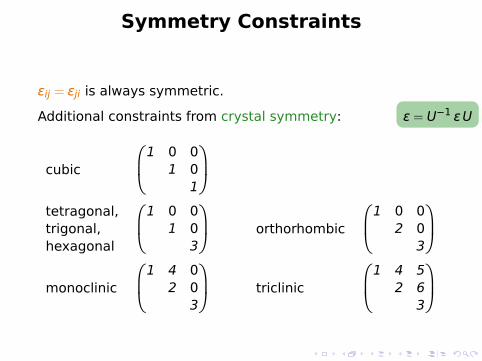
Symmetry Constraints
ϵij = ϵji is always symmetric.
Additional constraints from crystal symmetry: ϵ = U−1 ϵU
cubic
1 0 01 0
1
tetragonal,trigonal,hexagonal
1 0 01 0
3
orthorhombic
1 0 02 0
3
monoclinic
1 4 02 0
3
triclinic
1 4 52 6
3
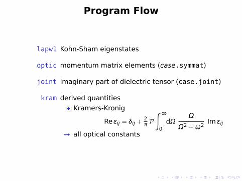
Program Flow
lapw1 Kohn-Sham eigenstates
optic momentum matrix elements (case.symmat)
joint imaginary part of dielectric tensor (case.joint)
kram derived quantities Kramers-Kronig
Re ϵij = δij +2π P∫ ∞
0dΩ
Ω
Ω2 −ω2Im ϵij
all optical constants
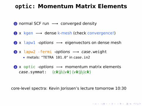
optic: Momentum Matrix Elements
0 normal SCF run −→ converged density
1 x kgen −→ dense k-mesh (check convergence!)
2 x lapw1 -options −→ eigenvectors on dense mesh
3 x lapw2 -fermi -options −→ case.weight metals: “TETRA 101.0” in case.in2
4 x optic -options −→ momentum matrix elementscase.symmat: ⟨ck|bpi|vk⟩ ⟨vk|bpj|ck⟩
core-level spectra: Kevin Jorissen’s lecture tomorrow 10:30
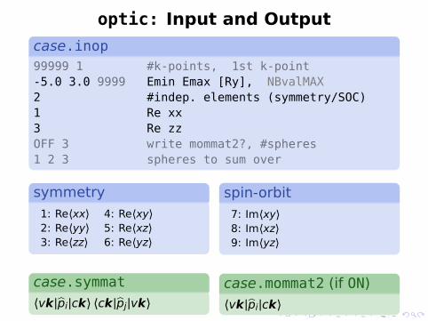
optic: Input and Outputcase.inop99999 1 #k-points, 1st k-point-5.0 3.0 9999 Emin Emax [Ry], NBvalMAX2 #indep. elements (symmetry/SOC)1 Re xx3 Re zzOFF 3 write mommat2?, #spheres1 2 3 spheres to sum over
symmetry1: Re⟨xx⟩ 4: Re⟨xy⟩2: Re⟨yy⟩ 5: Re⟨xz⟩3: Re⟨zz⟩ 6: Re⟨yz⟩
case.symmat⟨vk|bpi|ck⟩ ⟨ck|bpj|vk⟩
spin-orbit7: Im⟨xy⟩8: Im⟨xz⟩9: Im⟨yz⟩
case.mommat2 (if ON)⟨vk|bpi|ck⟩
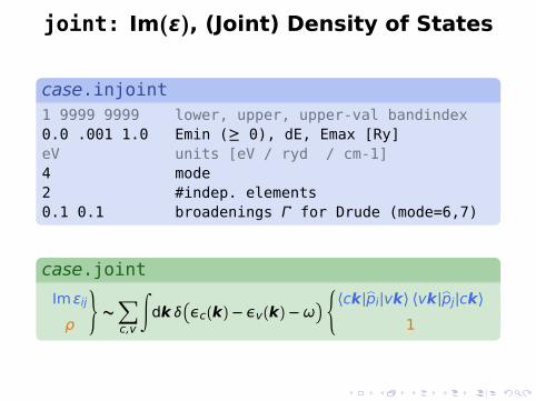
joint: Im(ϵ), (Joint) Density of States
case.injoint1 9999 9999 lower, upper, upper-val bandindex0.0 .001 1.0 Emin (≥ 0), dE, Emax [Ry]eV units [eV / ryd / cm-1]4 mode2 #indep. elements0.1 0.1 broadenings for Drude (mode=6,7)
case.joint
Im ϵij
ρ
)
∼∑
c,v
∫
dk δ
εc(k)− εv(k)−ω
(
⟨ck|bpi|vk⟩ ⟨vk|bpj|ck⟩
1
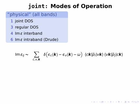
joint: Modes of Operation“physical” (all bands)
1 joint DOS
3 regular DOS
4 Im ϵ interband
6 Im ϵ intraband (Drude)
band analysis0 joint DOS
2 DOS
5 interband
7 intraband
Im ϵij ∼∑
c,v,k
δ
εc(k)− εv(k)−ω
⟨ck|bpi|vk⟩ ⟨vk|bpj|ck⟩
“sphere analysis”
|ck⟩ =MT,I∑
α|ck⟩α
NB: cross-terms are missed!
case.inopOFF 3 mommat2?, #spheres1 2 3 spheres to sum over
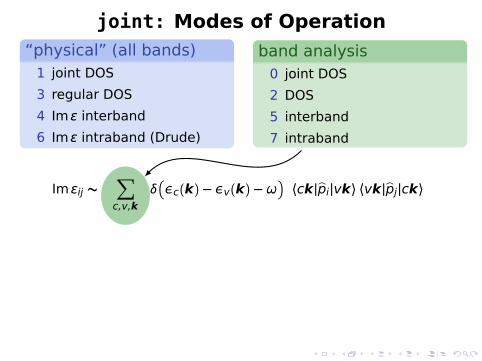
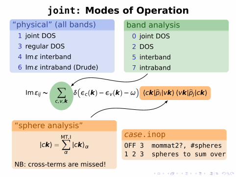
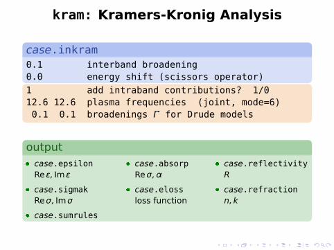
kram: Kramers-Kronig Analysis
case.inkram0.1 interband broadening0.0 energy shift (scissors operator)
1 add intraband contributions? 1/012.6 12.6 plasma frequencies (joint, mode=6)0.1 0.1 broadenings for Drude models
output case.epsilon
Re ϵ, Im ϵ
case.sigmakReσ, Imσ
case.sumrules
case.absorpReσ,α
case.elossloss function
case.reflectivityR
case.refractionn,k
More Stuff You May Need to Know
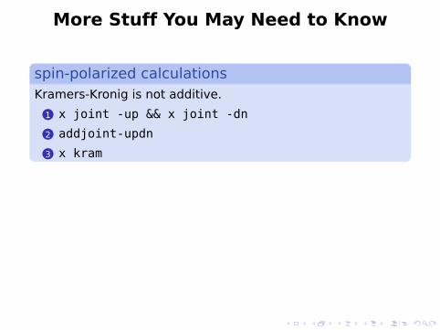
spin-polarized calculationsKramers-Kronig is not additive.
1 x joint -up && x joint -dn
2 addjoint-updn
3 x kram
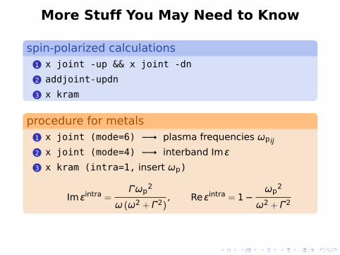
procedure for metals1 x joint (mode=6) −→ plasma frequencies ωpij
2 x joint (mode=4) −→ interband Im ϵ
3 x kram (intra=1, insert ωp)
More Stuff You May Need to Know
spin-polarized calculations1 x joint -up && x joint -dn
2 addjoint-updn
3 x kram
procedure for metals1 x joint (mode=6) −→ plasma frequencies ωpij
2 x joint (mode=4) −→ interband Im ϵ
3 x kram (intra=1, insert ωp)
Im ϵintra =ωp
2
ω (ω2 + 2), Re ϵintra = 1−
ωp2
ω2 + 2
More Stuff You May Need to Know
spin-polarized calculations1 x joint -up && x joint -dn
2 addjoint-updn
3 x kram
procedure for metals1 x joint (mode=6) −→ plasma frequencies ωpij
2 x joint (mode=4) −→ interband Im ϵ
3 x kram (intra=1, insert ωp)
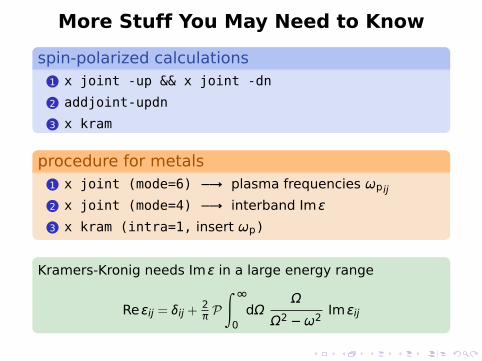
Kramers-Kronig needs Im ϵ in a large energy range
Re ϵij = δij +2π P∫ ∞
0dΩ
Ω
Ω2 −ω2Im ϵij
Some Limitations
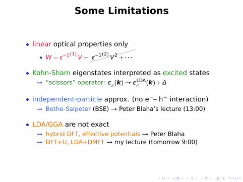
linear optical properties only
W = ϵ−1(1)V + ϵ−1(2)
V2 + · · ·
Kohn-Sham eigenstates interpreted as excited states “scissors” operator: εc(k)→ εLDA
c (k) + Δ
independent-particle approx. (no e−– h+ interaction) Bethe-Salpeter (BSE) → Peter Blaha’s lecture (13:00)
LDA/GGA are not exact hybrid DFT, effective potentials → Peter Blaha DFT+U, LDA+DMFT → my lecture (tomorrow 9:00)
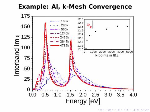
Example: Al, k-Mesh Convergence
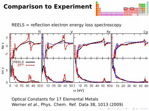
Comparison to Experiment
REELS = reflection electron energy loss spectroscopy
Optical Constants for 17 Elemental MetalsWerner et al., Phys. Chem. Ref. Data 38, 1013 (2009)
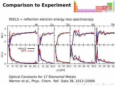
Comparison to Experiment
REELS = reflection electron energy loss spectroscopy
Optical Constants for 17 Elemental MetalsWerner et al., Phys. Chem. Ref. Data 38, 1013 (2009)
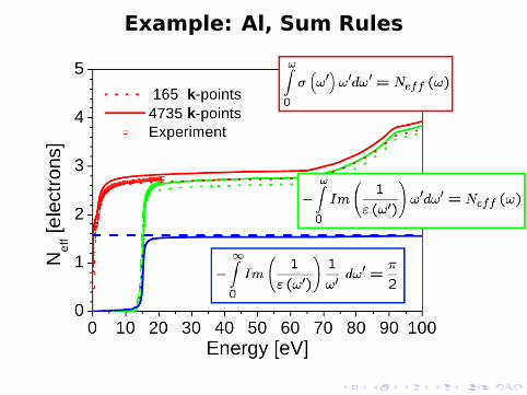
Example: Al, Sum Rules
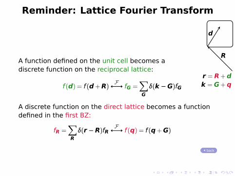
Reminder: Lattice Fourier Transform
R
d
r = R+dk =G+q
A function defined on the unit cell becomes adiscrete function on the reciprocal lattice:
f (d) = f (d+R)F←→ fG =∑
G
δ(k −G)fG
A discrete function on the direct lattice becomes a functiondefined in the first BZ:
fR =∑
R
δ(r −R)fRF←→ f (q) = f (q+G)
back