One-sample normal hypothesis Testing, paired t...
27
One-sample normal hypothesis Testing, paired t-test, two-sample normal inference, normal probability plots Timothy Hanson Department of Statistics, University of South Carolina Stat 704: Data Analysis I 1 / 27
-
Upload
nguyenliem -
Category
Documents
-
view
227 -
download
0
Transcript of One-sample normal hypothesis Testing, paired t...
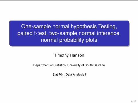
One-sample normal hypothesis Testing,paired t-test, two-sample normal inference,
normal probability plots
Timothy Hanson
Department of Statistics, University of South Carolina
Stat 704: Data Analysis I
1 / 27
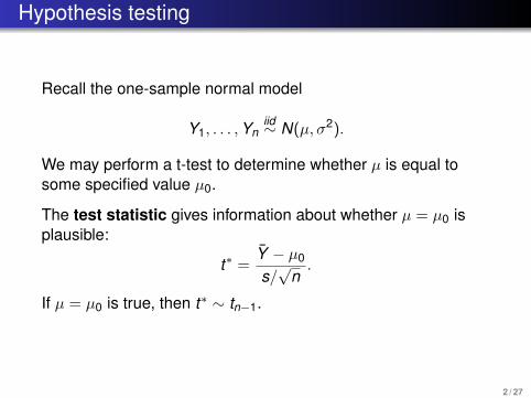
Hypothesis testing
Recall the one-sample normal model
Y1, . . . ,Yniid∼ N(µ, σ2).
We may perform a t-test to determine whether µ is equal tosome specified value µ0.
The test statistic gives information about whether µ = µ0 isplausible:
t∗ =Y − µ0
s/√
n.
If µ = µ0 is true, then t∗ ∼ tn−1.
2 / 27
Hypothesis testing
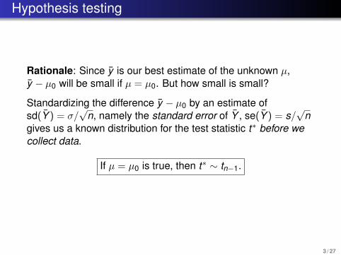
Rationale: Since y is our best estimate of the unknown µ,y − µ0 will be small if µ = µ0. But how small is small?
Standardizing the difference y − µ0 by an estimate ofsd(Y ) = σ/
√n, namely the standard error of Y , se(Y ) = s/
√n
gives us a known distribution for the test statistic t∗ before wecollect data.
If µ = µ0 is true, then t∗ ∼ tn−1.
3 / 27
Three types of test
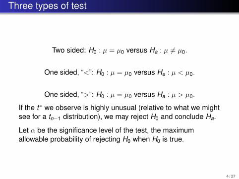
Two sided: H0 : µ = µ0 versus Ha : µ 6= µ0.
One sided, “<”: H0 : µ = µ0 versus Ha : µ < µ0.
One sided, “>”: H0 : µ = µ0 versus Ha : µ > µ0.
If the t∗ we observe is highly unusual (relative to what we mightsee for a tn−1 distribution), we may reject H0 and conclude Ha.
Let α be the significance level of the test, the maximumallowable probability of rejecting H0 when H0 is true.
4 / 27
Rejection rules
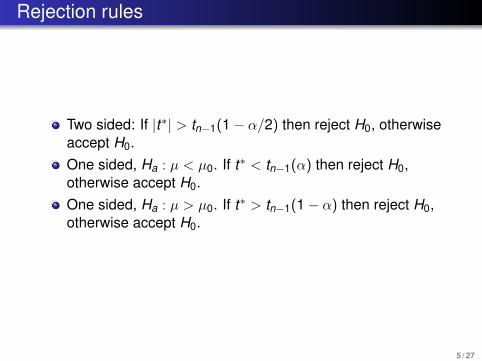
Two sided: If |t∗| > tn−1(1− α/2) then reject H0, otherwiseaccept H0.One sided, Ha : µ < µ0. If t∗ < tn−1(α) then reject H0,otherwise accept H0.One sided, Ha : µ > µ0. If t∗ > tn−1(1− α) then reject H0,otherwise accept H0.
5 / 27
p-value approach
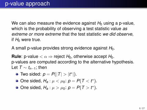
We can also measure the evidence against H0 using a p-value,which is the probability of observing a test statistic value asextreme or more extreme that the test statistic we did observe,if H0 were true.
A small p-value provides strong evidence against H0.
Rule: p-value < α⇒ reject H0, otherwise accept H0.p-values are computed according to the alternative hypothesis.Let T ∼ tn−1; then
Two sided: p = P(|T | > |t∗|).One sided, Ha : µ < µ0: p = P(T < t∗).One sided, Ha : µ > µ0: p = P(T > t∗).
6 / 27
Example
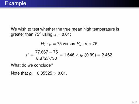
We wish to test whether the true mean high temperature isgreater than 75o using α = 0.01:
H0 : µ = 75 versus Ha : µ > 75.
t∗ =77.667− 758.872/
√30
= 1.646 < t29(0.99) = 2.462.
What do we conclude?
Note that p = 0.05525 > 0.01.
7 / 27
Connection between CI and two-sided test
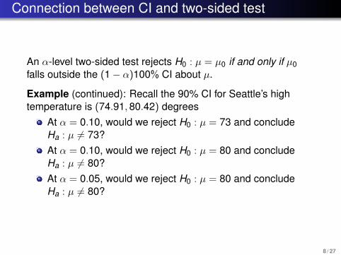
An α-level two-sided test rejects H0 : µ = µ0 if and only if µ0falls outside the (1− α)100% CI about µ.
Example (continued): Recall the 90% CI for Seattle’s hightemperature is (74.91,80.42) degrees
At α = 0.10, would we reject H0 : µ = 73 and concludeHa : µ 6= 73?At α = 0.10, would we reject H0 : µ = 80 and concludeHa : µ 6= 80?At α = 0.05, would we reject H0 : µ = 80 and concludeHa : µ 6= 80?
8 / 27
Paired data
When we have two paired samples (when each observation inone sample can be naturally paired with an observation in theother sample), we can use one-sample methods to obtaininference on the mean difference.
Example: n = 7 pairs of mice were injected with a cancer cell.Mice within each pair came from the same litter and weretherefore biologically similar. For each pair, one mouse wasgiven an experimental drug and the other mouse wasuntreated. After a time, the mice were sacrificed and thetumors weighed.
9 / 27
One-sample inference on differences
Let (Y1j ,Y2j) be the pair of control and treatment mice withinlitter j , j = 1, . . . ,7.
The difference in control versus treatment within each litter is
Dj = Y1j − Y2j .
If the differences follow a normal distribution, then we have themodel
Dj = µD + εj , j = 1, . . . ,n, where ε1, . . . , εniid∼ N(0, σ2).
Note that µD is the mean difference.
To test whether the control results in a higher mean tumorweight, form
H0 : µD = 0 versus Ha : µD > 0.
10 / 27
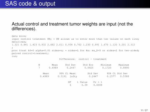
SAS code & output
Actual control and treatment tumor weights are input (not thedifferences).data mice;input control treatment @@; * @@ allows us to enter more than two values on each line;datalines;1.321 0.841 1.423 0.932 2.682 2.011 0.934 0.762 1.230 0.991 1.670 1.120 3.201 2.312;proc ttest h0=0 alpha=0.01 sides=u; * sides=L for Ha: mu_D<0 or sides=2 for two-sided;paired control*treatment;run;
Difference: control - treatment
N Mean Std Dev Std Err Minimum Maximum7 0.4989 0.2447 0.0925 0.1720 0.8890
Mean 95% CL Mean Std Dev 95% CL Std Dev0.4989 0.3191 Infty 0.2447 0.1577 0.5388
DF t Value Pr > t6 5.39 0.0008
11 / 27
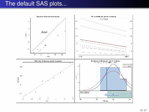
The default SAS plots...
12 / 27
Paired example, continued...
We’ll discuss the histogram and the Q-Q plot shortly...
For this test, the p-value is 0.0008. At α = 0.05, we reject H0and conclude that the true mean difference is larger than 0.
Restated: the treatment produces a significantly lower meantumor weight.
A 95% CI for the true mean difference µD is (0.27,0.73) (re-runwith sides=2). The mean tumor weight for untreated mice isbetween 0.27 and 0.73 grams higher than for treated mice.
13 / 27
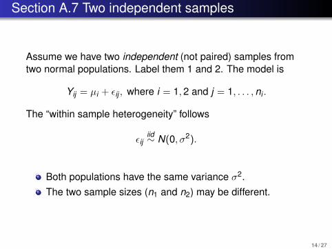
Section A.7 Two independent samples
Assume we have two independent (not paired) samples fromtwo normal populations. Label them 1 and 2. The model is
Yij = µi + εij , where i = 1,2 and j = 1, . . . ,ni .
The “within sample heterogeneity” follows
εijiid∼ N(0, σ2).
Both populations have the same variance σ2.The two sample sizes (n1 and n2) may be different.
14 / 27
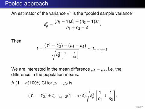
Pooled approach
An estimator of the variance σ2 is the “pooled sample variance”
s2p =
(n1 − 1)s21 + (n2 − 1)s2
2n1 + n2 − 2
.
Then
t =(Y1 − Y2)− (µ1 − µ2)√
s2p
[1n1
+ 1n2
] ∼ tn1+n2−2.
We are interested in the mean difference µ1 − µ2, i.e. thedifference in the population means.
A (1− α)100% CI for µ1 − µ2 is
(Y1 − Y2)± tn1+n2−2(1− α/2)
√s2
p
[1n1
+1n2
].
15 / 27
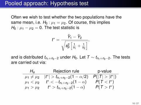
Pooled approach: Hypothesis test
Often we wish to test whether the two populations have thesame mean, i.e. H0 : µ1 = µ2. Of course, this impliesH0 : µ1 − µ2 = 0. The test statistic is
t∗ =Y1 − Y2√
s2p
[1n1
+ 1n2
] ,and is distributed tn1+n2−2 under H0. Let T ∼ tn1+n2−2. The testsare carried out via:
Ha Rejection rule p-valueµ1 6= µ2 |t∗| > tn1+n2−2(1− α/2) P(|T | > |t∗|)µ1 < µ2 t∗ < −tn1+n2−2(1− α) P(T < t∗)µ1 > µ2 t∗ > tn1+n2−2(1− α) P(T > t∗)
16 / 27
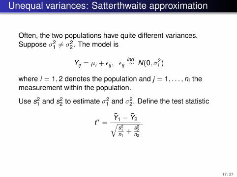
Unequal variances: Satterthwaite approximation
Often, the two populations have quite different variances.Suppose σ2
1 6= σ22. The model is
Yij = µi + εij , εijind .∼ N(0, σ2
i )
where i = 1,2 denotes the population and j = 1, . . . ,ni themeasurement within the population.
Use s21 and s2
2 to estimate σ21 and σ2
2. Define the test statistic
t∗ =Y1 − Y2√
s21
n1+
s22
n2
.
17 / 27
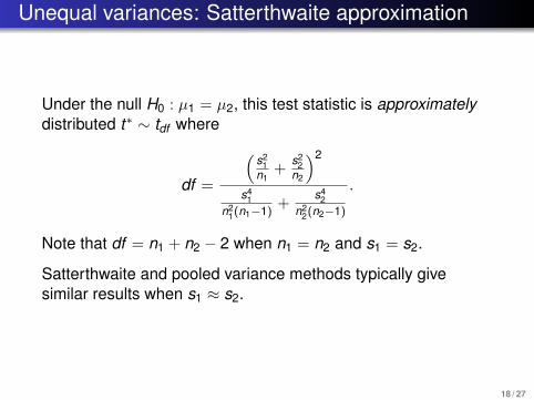
Unequal variances: Satterthwaite approximation
Under the null H0 : µ1 = µ2, this test statistic is approximatelydistributed t∗ ∼ tdf where
df =
(s2
1n1
+s2
2n2
)2
s41
n21(n1−1) +
s42
n22(n2−1)
.
Note that df = n1 + n2 − 2 when n1 = n2 and s1 = s2.
Satterthwaite and pooled variance methods typically givesimilar results when s1 ≈ s2.
18 / 27
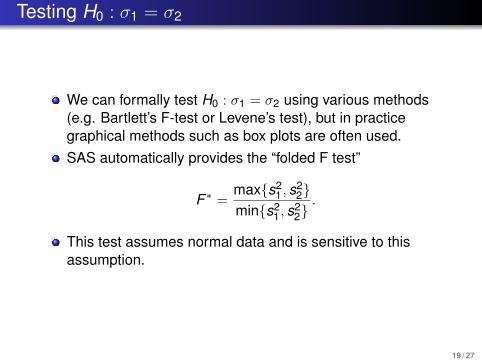
Testing H0 : σ1 = σ2
We can formally test H0 : σ1 = σ2 using various methods(e.g. Bartlett’s F-test or Levene’s test), but in practicegraphical methods such as box plots are often used.SAS automatically provides the “folded F test”
F ∗ =max{s2
1, s22}
min{s21, s
22}.
This test assumes normal data and is sensitive to thisassumption.
19 / 27

SAS example
Example: Data were collected on pollution around a chemicalplant (Rao, p. 137). Two independent samples of river waterwere taken, one upstream and one downstream. Pollution levelwas measured in ppm. Do the mean pollution levels differ atα = 0.05?SAS codedata pollution;input level location $ @@; * use $ to denote a categorical variable;datalines;24.5 up 29.7 up 20.4 up 28.5 up 25.3 up 21.8 up 20.2 up 21.0 up21.9 up 22.2 up 32.8 down 30.4 down 32.3 down 26.4 down 27.8 down 26.9 down29.0 down 31.5 down 31.2 down 26.7 down 25.6 down 25.1 down 32.8 down 34.3 down35.4 down;
proc ttest h0=0 alpha=0.05 sides=2;class location; var level;
run;
20 / 27
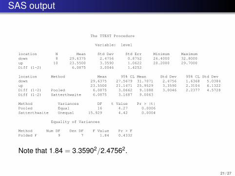
SAS output
The TTEST Procedure
Variable: level
location N Mean Std Dev Std Err Minimum Maximumdown 8 29.6375 2.4756 0.8752 26.4000 32.8000up 10 23.5500 3.3590 1.0622 20.2000 29.7000Diff (1-2) 6.0875 3.0046 1.4252
location Method Mean 95% CL Mean Std Dev 95% CL Std Devdown 29.6375 27.5679 31.7071 2.4756 1.6368 5.0384up 23.5500 21.1471 25.9529 3.3590 2.3104 6.1322Diff (1-2) Pooled 6.0875 3.0662 9.1088 3.0046 2.2377 4.5728Diff (1-2) Satterthwaite 6.0875 3.1687 9.0063
Method Variances DF t Value Pr > |t|Pooled Equal 16 4.27 0.0006Satterthwaite Unequal 15.929 4.42 0.0004
Equality of Variances
Method Num DF Den DF F Value Pr > FFolded F 9 7 1.84 0.4332
Note that 1.84 = 3.35902/2.47562.
21 / 27
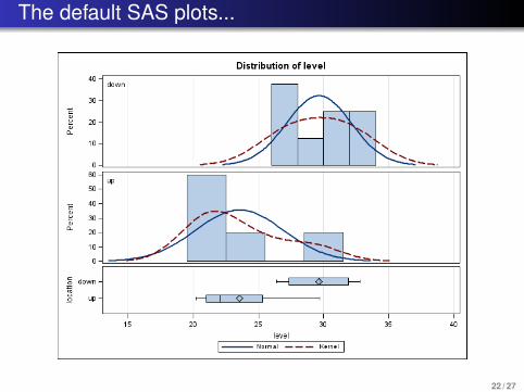
The default SAS plots...
22 / 27
The default SAS plots...
23 / 27
Assumptions going into t procedures
Note: Recall our t-procedures require that the data come fromnormal population(s).
Fortunately, the t procedures are robust: they workapproximately correctly if the population distribution is “close” tonormal.
Also, if our sample sizes are large, we can use the t procedures(or simply normal-based procedures) even if our data are notnormal because of the central limit theorem.
If the sample size is small, we should perform some check ofnormality to ensure t tests and CIs are okay.
Question: Are there any other assumptions going into themodel that can or should be checked or at least thought about?For example, what if pollution measurements were taken onconsecutive days?
24 / 27
Boxplots for checking normality
To use t tests and CIs in small samples, approximatenormality should be checked.Could check with a histogram or boxplot: verify distributionis approximately symmetric.Note: For perfectly normal data, the probability of seeingan outlier on an R or SAS boxplot using defaults is 0.0070.For a sample size ni = 150, in perfectly normal data weexpect to see 0.007(150) ≈ 1 outlier. Certainly for smallsample sizes, we expect to see none.
25 / 27
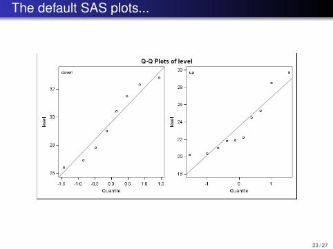
Q-Q plot for checking normality
More precise plot: normal Q-Q plot. Idea: the human eyeis very good at detecting deviations from linearity.Q-Q plot is ordered data against normal quantileszi = Φ−1{i/(n + 1)} for i = 1, . . . ,n.Idea: zi ≈ E(Z(i)), the expected order statistic understandard normal assumption.A plot of y(i) versus zi should be reasonably straight if dataare normal.However, in small sample sizes there is a lot of variability inthe plots even with perfectly normal data...
Example: R example of Q-Q plots and R code to examinenormal, skewed, heavy-tailed, and light-tailed distributions.Note both Q-Q plots and numbers of outliers on R boxplot.
26 / 27
Assumptions for two examples
Mice tumor data: Q-Q plot? Boxplot? Histogram?River water pollution data: Q-Q plots? Boxplots?Histograms?
Teaching effectiveness, continued...proc ttest h0=0 alpha=0.05 sides=2;class attend; var rating;
run;
27 / 27