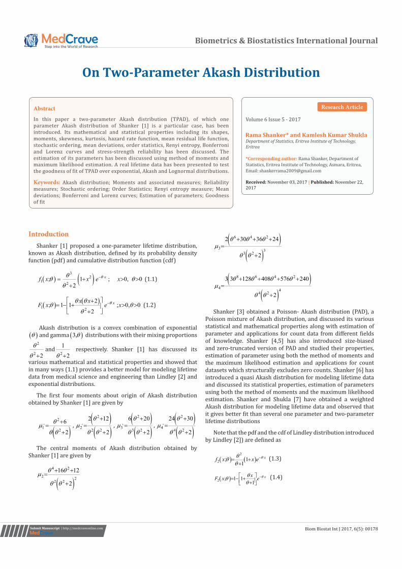
On Two-Parameter Akash Distribution - Medcravemedcraveonline.com/BBIJ/BBIJ-06-00178.pdf ·...
11
Biometrics & Biostatistics International Journal On Two-Parameter Akash Distribution Submit Manuscript | http://medcraveonline.com Introduction Shanker [1] proposed a one-parameter lifetime distribution, known as Akash distribution, defined by its probability density function (pdf) and cumulative distribution function (cdf) ( ) ( ) 3 2 1 2 ; 1 ; 0, 0 2 x f x x e x θ θ θ θ θ − = + > > + (1.1) ( ) ( ) 1 2 2 ; 1 1 ; 0, 0 2 x x x F x e x θ θ θ θ θ θ − + =− + > > + (1.2) Akash distribution is a convex combination of exponential ( ) θ and gamma ( ) 3, θ distributions with their mixing proportions 2 2 2 θ θ + and 2 1 2 θ + respectively. Shanker [1] has discussed its various mathematical and statistical properties and showed that in many ways (1.1) provides a better model for modeling lifetime data from medical science and engineering than Lindley [2] and exponential distributions. The first four moments about origin of Akash distribution obtained by Shanker [1] are given by ( ) 2 1 2 6 2 θ µ θθ ′ + = + , ( ) ( ) 2 2 2 2 2 12 2 θ µ θ θ ′ + = + , ( ) ( ) 2 3 3 2 6 20 2 θ µ θ θ ′ + = + , ( ) ( ) 2 4 4 2 24 30 2 θ µ θ θ ′ + = + The central moments of Akash distribution obtained by Shanker [1] are given by ( ) 4 2 2 2 2 2 16 12 2 θ θ µ θ θ + + = + ( ) ( ) 8 6 4 2 4 4 4 2 33 128 408 576 240 2 θ θ θ θ µ θ θ + + + + = + Shanker [3] obtained a Poisson- Akash distribution (PAD), a Poisson mixture of Akash distribution, and discussed its various statistical and mathematical properties along with estimation of parameter and applications for count data from different fields of knowledge. Shanker [4,5] has also introduced size-biased and zero-truncated version of PAD and studied their properties, estimation of parameter using both the method of moments and the maximum likelihood estimation and applications for count datasets which structurally excludes zero counts. Shanker [6] has introduced a quasi Akash distribution for modeling lifetime data and discussed its statistical properties, estimation of parameters using both the method of moments and the maximum likelihood estimation. Shanker and Shukla [7] have obtained a weighted Akash distribution for modeling lifetime data and observed that it gives better fit than several one parameter and two-parameter lifetime distributions Note that the pdf and the cdf of Lindley distribution introduced by Lindley [2]) are defined as ( ) ( ) 2 2 ; 1 1 x f x xe θ θ θ θ − = + + (1.3) ( ) 2 ; 1 1 1 x x F x e θ θ θ θ − =− + + (1.4) Volume 6 Issue 5 - 2017 Department of Statistics, Eritrea Institute of Technology, Eritrea *Corresponding author: Rama Shanker, Department of Statistics, Eritrea Institute of Technology, Asmara, Eritrea, Email: Received: November 03, 2017 | Published: November 22, 2017 Research Article Biom Biostat Int J 2017, 6(5): 00178 Abstract In this paper a two-parameter Akash distribution (TPAD), of which one parameter Akash distribution of Shanker [1] is a particular case, has been introduced. Its mathematical and statistical properties including its shapes, moments, skewness, kurtosis, hazard rate function, mean residual life function, stochastic ordering, mean deviations, order statistics, Renyi entropy, Bonferroni and Lorenz curves and stress-strength reliability has been discussed. The estimation of its parameters has been discussed using method of moments and maximum likelihood estimation. A real lifetime data has been presented to test the goodness of fit of TPAD over exponential, Akash and Lognormal distributions. Keywords: Akash distribution; Moments and associated measures; Reliability measures; Stochastic ordering; Order Statistics; Renyi entropy measure; Mean deviations; Bonferroni and Lorenz curves; Estimation of parameters; Goodness of fit ( ) ( ) 6 4 2 3 3 3 2 2 30 36 24 2 θ θ θ µ θ θ + + + = +
Transcript of On Two-Parameter Akash Distribution - Medcravemedcraveonline.com/BBIJ/BBIJ-06-00178.pdf ·...
Biometrics & Biostatistics International Journal
On Two-Parameter Akash Distribution
Submit Manuscript | http://medcraveonline.com
Introduction Shanker [1] proposed a one-parameter lifetime distribution,
known as Akash distribution, defined by its probability density function (pdf) and cumulative distribution function (cdf)
( ) ( )32
1 2; 1 ; 0, 0
2xf x x e xθθθ θ
θ−= + > >
+ (1.1)
( ) ( )1 2
2; 1 1 ; 0, 0
2xx x
F x e xθθ θθ θ
θ− +
= − + > > +
(1.2)
Akash distribution is a convex combination of exponential( )θ and gamma ( )3,θ distributions with their mixing proportions
2
2 2
θ
θ +and
2
1
2θ + respectively. Shanker [1] has discussed its
various mathematical and statistical properties and showed that in many ways (1.1) provides a better model for modeling lifetime data from medical science and engineering than Lindley [2] and exponential distributions.
The first four moments about origin of Akash distribution obtained by Shanker [1] are given by
( )
2
1 2
6
2
θµθ θ
′+
=+
, ( )( )
2
2 2 2
2 12
2
θµ
θ θ′
+=
+,
( )( )
2
3 3 2
6 20
2
θµ
θ θ′
+=
+,
( )( )
2
4 4 2
24 30
2
θµ
θ θ′
+=
+
The central moments of Akash distribution obtained by Shanker [1] are given by
( )4 2
2 22 2
16 12
2
θ θµθ θ
+ +=
+
( )( )
8 6 4 2
4 44 2
3 3 128 408 576 240
2
θ θ θ θµ
θ θ
+ + + +=
+ Shanker [3] obtained a Poisson- Akash distribution (PAD), a
Poisson mixture of Akash distribution, and discussed its various statistical and mathematical properties along with estimation of parameter and applications for count data from different fields of knowledge. Shanker [4,5] has also introduced size-biased and zero-truncated version of PAD and studied their properties, estimation of parameter using both the method of moments and the maximum likelihood estimation and applications for count datasets which structurally excludes zero counts. Shanker [6] has introduced a quasi Akash distribution for modeling lifetime data and discussed its statistical properties, estimation of parameters using both the method of moments and the maximum likelihood estimation. Shanker and Shukla [7] have obtained a weighted Akash distribution for modeling lifetime data and observed that it gives better fit than several one parameter and two-parameter lifetime distributions
Note that the pdf and the cdf of Lindley distribution introduced by Lindley [2]) are defined as
( ) ( )
2
2 ; 11
xf x x e θθθθ
−= ++
(1.3)
( )2 ; 1 1
1xxF x e θθθ
θ− = − + +
(1.4)
Volume 6 Issue 5 - 2017
Department of Statistics, Eritrea Institute of Technology, Eritrea
*Corresponding author: Rama Shanker, Department of Statistics, Eritrea Institute of Technology, Asmara, Eritrea, Email:
Received: November 03, 2017 | Published: November 22, 2017
Research Article
Biom Biostat Int J 2017, 6(5): 00178
Abstract
In this paper a two-parameter Akash distribution (TPAD), of which one parameter Akash distribution of Shanker [1] is a particular case, has been introduced. Its mathematical and statistical properties including its shapes, moments, skewness, kurtosis, hazard rate function, mean residual life function, stochastic ordering, mean deviations, order statistics, Renyi entropy, Bonferroni and Lorenz curves and stress-strength reliability has been discussed. The estimation of its parameters has been discussed using method of moments and maximum likelihood estimation. A real lifetime data has been presented to test the goodness of fit of TPAD over exponential, Akash and Lognormal distributions.
Keywords: Akash distribution; Moments and associated measures; Reliability measures; Stochastic ordering; Order Statistics; Renyi entropy measure; Mean deviations; Bonferroni and Lorenz curves; Estimation of parameters; Goodness of fit
( )( )
6 4 2
3 33 2
2 30 36 24
2
θ θ θµ
θ θ
+ + +=
+
Citation: Shanker R, Shukla KK (2017) On Two-Parameter Akash Distribution. Biom Biostat Int J 6(5): 00178. DOI: 10.15406/bbij.2017.06.00178
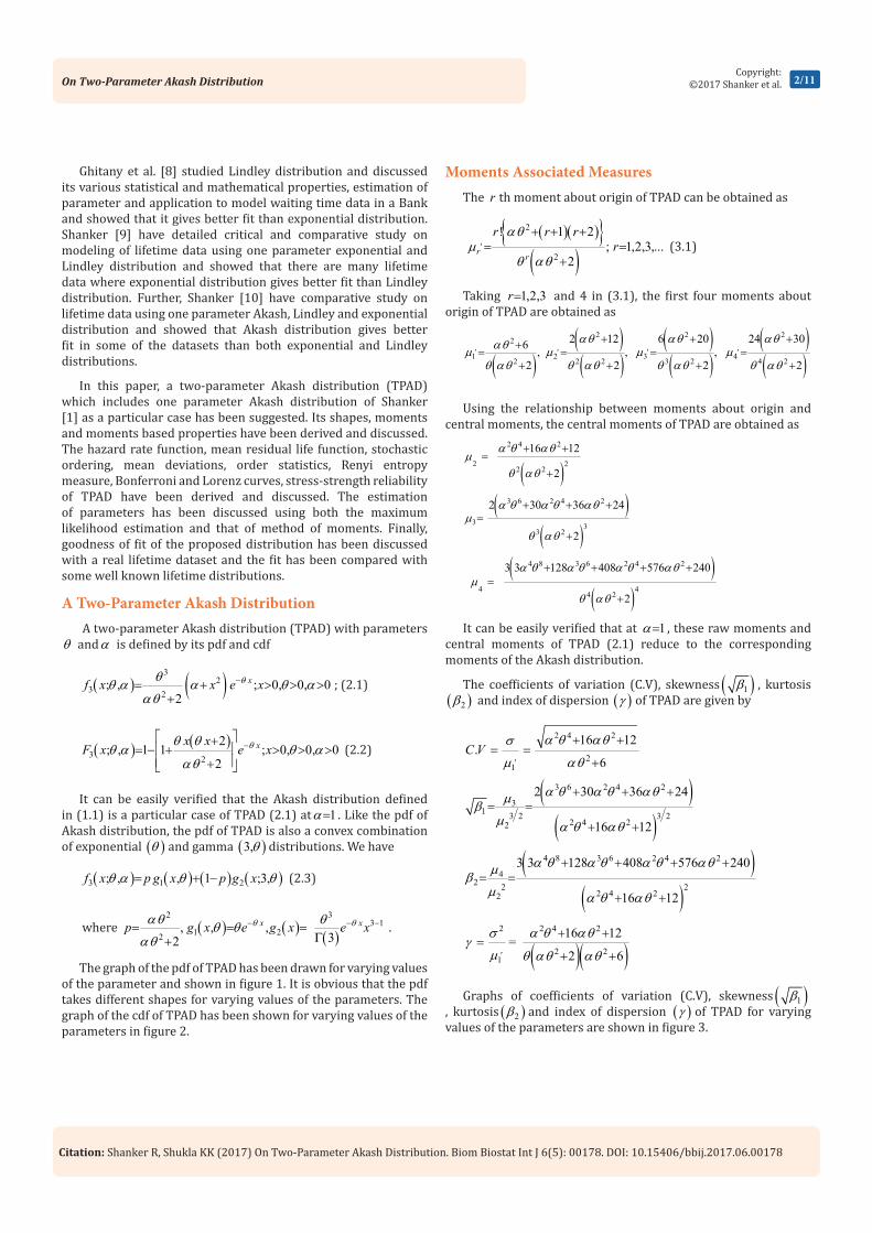
On Two-Parameter Akash Distribution 2/11Copyright:
©2017 Shanker et al.
Ghitany et al. [8] studied Lindley distribution and discussed its various statistical and mathematical properties, estimation of parameter and application to model waiting time data in a Bank and showed that it gives better fit than exponential distribution. Shanker [9] have detailed critical and comparative study on modeling of lifetime data using one parameter exponential and Lindley distribution and showed that there are many lifetime data where exponential distribution gives better fit than Lindley distribution. Further, Shanker [10] have comparative study on lifetime data using one parameter Akash, Lindley and exponential distribution and showed that Akash distribution gives better fit in some of the datasets than both exponential and Lindley distributions.
In this paper, a two-parameter Akash distribution (TPAD) which includes one parameter Akash distribution of Shanker [1] as a particular case has been suggested. Its shapes, moments and moments based properties have been derived and discussed. The hazard rate function, mean residual life function, stochastic ordering, mean deviations, order statistics, Renyi entropy measure, Bonferroni and Lorenz curves, stress-strength reliability of TPAD have been derived and discussed. The estimation of parameters has been discussed using both the maximum likelihood estimation and that of method of moments. Finally, goodness of fit of the proposed distribution has been discussed with a real lifetime dataset and the fit has been compared with some well known lifetime distributions.
A Two-Parameter Akash Distribution A two-parameter Akash distribution (TPAD) with parameters
θ andα is defined by its pdf and cdf
( ) ( )3
23 2
; , ; 0, 0, 02
xf x x e xθθθ α α θ ααθ
−= + > > >+
; (2.1)
( ) ( )
3 2
2; , 1 1 ; 0, 0, 0
2xx x
F x e xθθ θθ α θ α
αθ−
+ = − + > > > +
(2.2)
It can be easily verified that the Akash distribution defined in (1.1) is a particular case of TPAD (2.1) at 1α= . Like the pdf of Akash distribution, the pdf of TPAD is also a convex combination of exponential ( )θ and gamma ( )3,θ distributions. We have
( ) ( ) ( ) ( )3 1 2; , , 1 ;3,f x p g x p g xθ α θ θ= + − (2.3)
where ( ) ( ) ( )2 3
3 11 22
, , ,32
x xp g x e g x e xθ θαθ θθ θαθ
− − −= = =Γ+
.
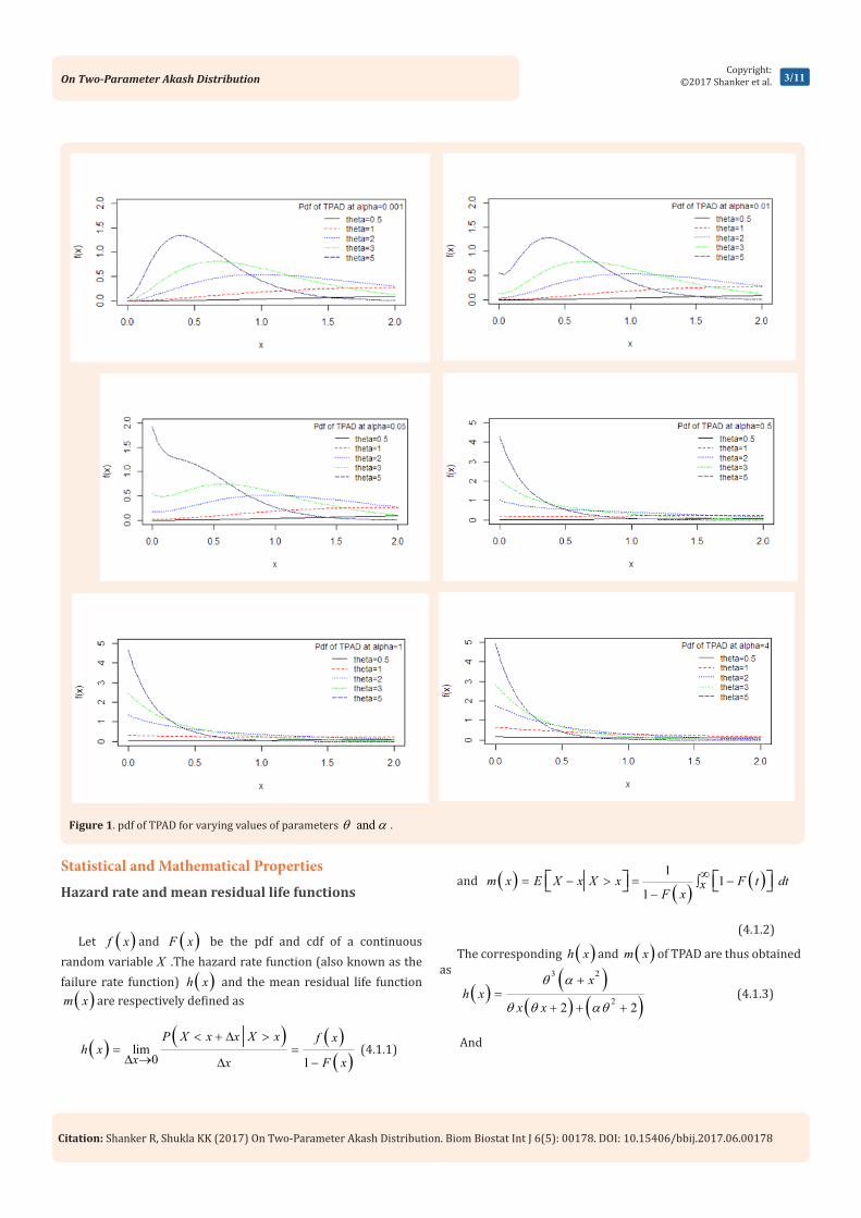
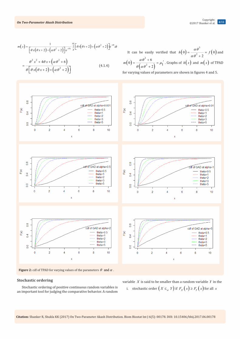
The graph of the pdf of TPAD has been drawn for varying values of the parameter and shown in figure 1. It is obvious that the pdf takes different shapes for varying values of the parameters. The graph of the cdf of TPAD has been shown for varying values of the parameters in figure 2.
Moments Associated MeasuresThe r th moment about origin of TPAD can be obtained as
( )( ){ }
( )2
2
! 1 2; 1,2,3,...
2r r
r r rr
αθµ
θ αθ′
+ + += =
+ (3.1)
Taking 1,2,3r= and 4 in (3.1), the first four moments about origin of TPAD are obtained as
( )
( )( )
( )( )
( )( )
2 2 22
1 2 3 42 2 2 3 2 4 2
2 12 6 20 24 306 , , , 2 2 2 2
αθ αθ αθαθµ µ µ µθ αθ θ αθ θ αθ θ αθ
′ ′ ′ ′+ + ++
= = = =+ + + +
Using the relationship between moments about origin and
central moments, the central moments of TPAD are obtained as
( )( )
( )( )
( )
2 4 2
2 22 2
3 6 2 4 2
3 33 2
4 8 3 6 2 4 2
4 44 2
16 12
2
2 30 36 24
2
3 3 128 408 576 240
2
α θ αθµ
θ αθ
α θ α θ αθµ
θ αθ
α θ α θ α θ αθµ
θ αθ
+ +=
+
+ + +=
+
+ + + +=
+
It can be easily verified that at 1α= , these raw moments and central moments of TPAD (2.1) reduce to the corresponding moments of the Akash distribution.
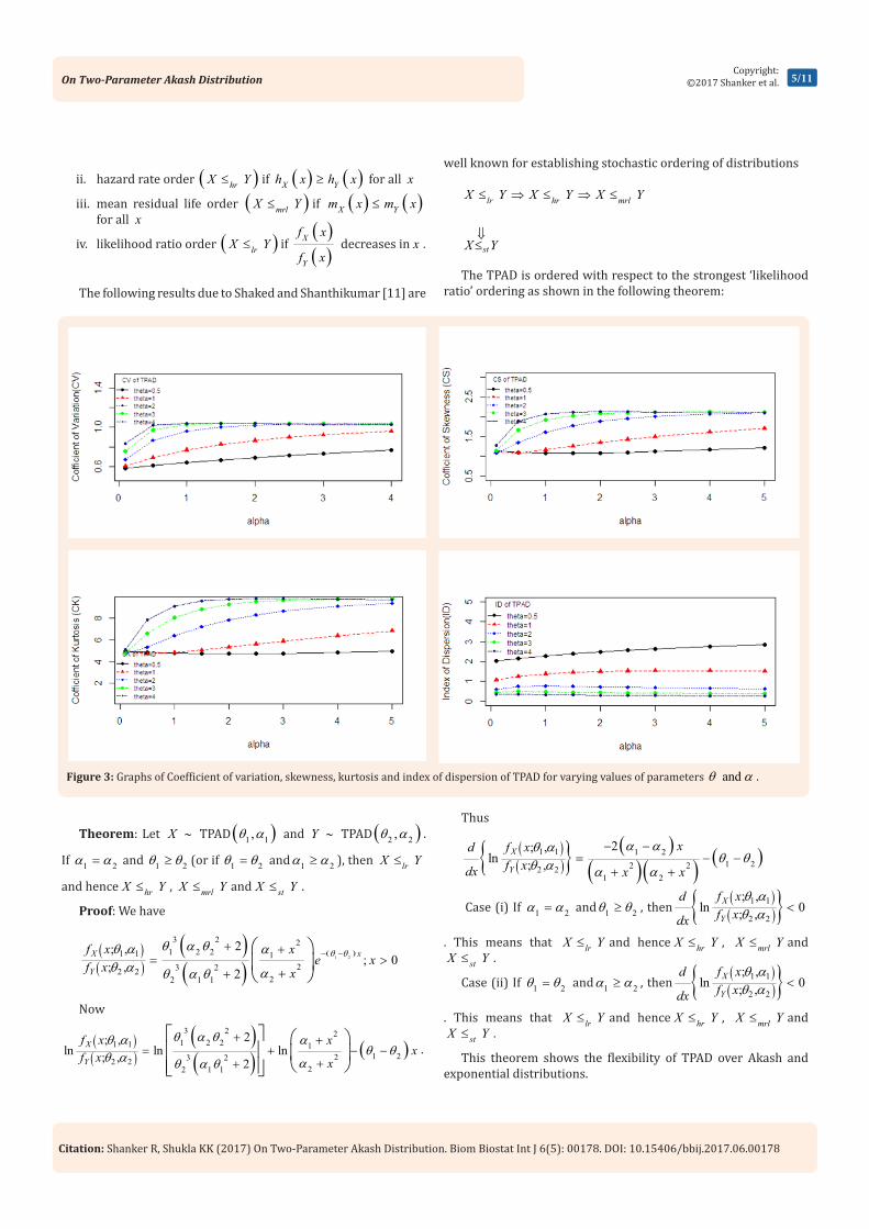
The coefficients of variation (C.V), skewness ( )1β , kurtosis( )2β and index of dispersion ( )γ of TPAD are given by
( )( )
( )( )
( )( )
2 4 2
21
3 6 2 4 2
31 3 2 3 2
2 4 22
4 8 3 6 2 4 2
42 2 2
2 4 22
2 2 4 2
2 21
16 12.
6
2 30 36 24
16 12
3 3 128 408 576 240
16 12
16 12=
2 6
C Vα θ αθσ
µ αθ
α θ α θ αθµβµ α θ αθ
α θ α θ α θ αθµβµ α θ αθ
σ α θ αθγ
µ θ αθ αθ
′
′
+ += =
+
+ + += =
+ +
+ + + += =
+ +
+ +=
+ +
Graphs of coefficients of variation (C.V), skewness ( )1β, kurtosis ( )2β and index of dispersion ( )γ of TPAD for varying values of the parameters are shown in figure 3.
2/11
Citation: Shanker R, Shukla KK (2017) On Two-Parameter Akash Distribution. Biom Biostat Int J 6(5): 00178. DOI: 10.15406/bbij.2017.06.00178
On Two-Parameter Akash Distribution 3/11Copyright:
©2017 Shanker et al.
Figure 1. pdf of TPAD for varying values of parameters andθ α .
Statistical and Mathematical Properties
Hazard rate and mean residual life functions
Let ( )f x and ( )F x be the pdf and cdf of a continuous random variable X .The hazard rate function (also known as the failure rate function) ( )h x and the mean residual life function ( )m x are respectively defined as
( ) ( ) ( )( )
lim0 1
P X x x X x f xh x
x x F x
< + ∆ >= =∆ → ∆ −
(4.1.1)
and ( ) ( ) ( )1 1
1m x E X x X x F t dtx
F x∞= − > = −∫
−
(4.1.2)
The corresponding ( )h x and ( )m x of TPAD are thus obtained as
( ) ( )( ) ( )
3 2
22 2
xh x
x x
θ α
θ θ αθ
+=
+ + + (4.1.3)
And
Citation: Shanker R, Shukla KK (2017) On Two-Parameter Akash Distribution. Biom Biostat Int J 6(5): 00178. DOI: 10.15406/bbij.2017.06.00178
On Two-Parameter Akash Distribution 4/11Copyright:
©2017 Shanker et al.
( )
( ) ( ) ( ) ( )2
2
12 2
2 2
t
xm x t t e dt
xx x e
θ
θθ θ αθ
θ θ αθ
−
−
∞= + + +∫
+ + +
( )( ) ( )
2 2 2
2
4 6
2 2
x x
x x
θ θ αθ
θ θ θ αθ
+ + +=
+ + + (4.1.4)
It can be easily verified that ( ) ( )3
20 02
h fαθ
αθ= =
+and
( ) ( )2
2
60 12
mαθ
µθ αθ
+ ′= =+
. Graphs of ( )h x and ( )m x of TPAD
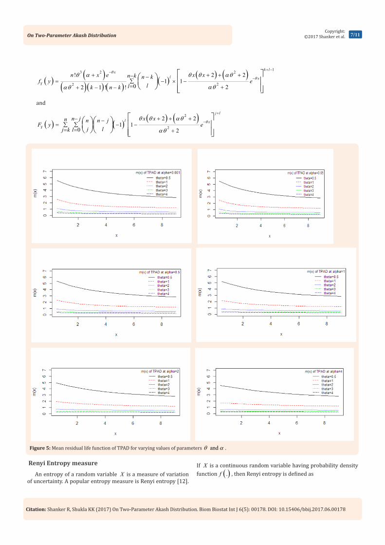
for varying values of parameters are shown in figures 4 and 5.
Figure 2: cdf of TPAD for varying values of the parameters andθ α .
Stochastic ordering
Stochastic ordering of positive continuous random variables is an important tool for judging the comparative behavior. A random
variable X is said to be smaller than a random variable Y in the
i. stochastic order ( )stX Y≤ if ( ) ( )X YF x F x≥ for all x
Citation: Shanker R, Shukla KK (2017) On Two-Parameter Akash Distribution. Biom Biostat Int J 6(5): 00178. DOI: 10.15406/bbij.2017.06.00178
On Two-Parameter Akash Distribution 5/11Copyright:
©2017 Shanker et al.
ii. hazard rate order ( )hrX Y≤ if ( ) ( )X Yh x h x≥ for all x
iii. mean residual life order ( )mrlX Y≤ if ( ) ( )X Ym x m x≤for all x
iv. likelihood ratio order ( )lrX Y≤ if ( )( )
X
Y
f x
f x decreases in x .
The following results due to Shaked and Shanthikumar [11] are
well known for establishing stochastic ordering of distributions
lr hr mrlX Y X Y X Y≤ ⇒ ≤ ⇒ ≤
stX Y⇓≤
The TPAD is ordered with respect to the strongest ‘likelihood ratio’ ordering as shown in the following theorem:
Figure 3: Graphs of Coefficient of variation, skewness, kurtosis and index of dispersion of TPAD for varying values of parameters andθ α .
Theorem: Let X ∼ TPAD ( )1 1,θ α and Y ∼ TPAD ( )2 2,θ α .
If 1 2α α= and 1 2θ θ≥ (or if 1 2θ θ= and 1 2α α≥ ), then lrX Y≤
and hence hrX Y≤ , mrlX Y≤ and stX Y≤ .
Proof: We have
( )( )
( )( )
( )1 2
3 2 21 2 21 1 1
23 22 222 1 1
2; ,; 0; , 2
X x
Y
f x xe xf x x
θ θθ α θθ α α
θ α αθ α θ
− −+ +
= >++
Now
( )( )
( )( ) ( )
3 2 21 2 21 1 1
1 223 22 222 1 1
2; ,ln ln ln; , 2
X
Y
f x xxf x x
θ α θθ α αθ θθ α αθ α θ
+ += + − −
++
.
Thus
( )( ){ } ( )
( )( ) ( )1 1 1 21 22 22 2
1 2
2; ,ln ; ,
X
Y
xf xdf xdx x x
α αθ αθ θθ α α α
− −= − −
+ +
Case (i) If 1 2α α= and 1 2θ θ≥ , then( )( ){ }1 1
2 2
; ,ln 0; ,
X
Y
f xdf xdx
θ αθ α <
. This means that lrX Y≤ and hence hrX Y≤ , mrlX Y≤ andstX Y≤ .
Case (ii) If 1 2θ θ= and 1 2α α≥ , then( )( ){ }1 1
2 2
; ,ln 0; ,
X
Y
f xdf xdx
θ αθ α <
. This means that lrX Y≤ and hence hrX Y≤ , mrlX Y≤ andstX Y≤ .
This theorem shows the flexibility of TPAD over Akash and exponential distributions.

Citation: Shanker R, Shukla KK (2017) On Two-Parameter Akash Distribution. Biom Biostat Int J 6(5): 00178. DOI: 10.15406/bbij.2017.06.00178
On Two-Parameter Akash Distribution 6/11Copyright:
©2017 Shanker et al.
Figure 4: Hazard rate function of TPAD for varying values of parameters andθ α .
Distribution of order statistics
Let 1 2, ,..., nX X X be a random sample of size n from TPAD. Let
( ) ( ) ( )1 2 ... nX X X< < < denote the corresponding order statistics. The pdf and the cdf of the k th order statistic, say ( )kY X= are given by
( ) ( ) ( ) ( ) ( ){ } ( )1!1
1 ! !
n kkY
nf y F y F y f y
k n k
−−= −− −
( ) ( ) ( ) ( ) ( )1!1
01 ! !
l k ln kn n kF y f y
llk n k+ −− −
∑= −=− −
and
( ) ( ) ( ){ }1n jj
Y
n nF y F y F y
jj k
−∑= −=
( ) ( )10
l j ln jn n n j
F yj lj k l
+− −
∑ ∑= −= =
,
respectively, for 1, 2, 3, ...,k n= .
Thus, the pdf and the cdf of k th order statistics of TPAD are obtained as
Citation: Shanker R, Shukla KK (2017) On Two-Parameter Akash Distribution. Biom Biostat Int J 6(5): 00178. DOI: 10.15406/bbij.2017.06.00178
On Two-Parameter Akash Distribution 7/11Copyright:
©2017 Shanker et al.
( ) ( )( )( ) ( )
( )( ) ( ) 1
3 2 2
22
! 2 21 1
0 22 1 ! !
k lxl x
Y
n x e x xn k n kf y e
llk n k
θθ
θ α θ θ αθ
αθαθ
+ −−
−+ + + +− −
∑= − × −= ++ − −
and
( ) ( )( ) ( )2
2
2 21 1
0 2
j l
l xY
x xn jn n n jF y e
j lj k lθ
θ θ αθ
αθ
+
−+ + +− −
∑ ∑= − −= = +
Figure 5: Mean residual life function of TPAD for varying values of parameters andθ α .
Renyi Entropy measure
An entropy of a random variable X is a measure of variation of uncertainty. A popular entropy measure is Renyi entropy [12].
If X is a continuous random variable having probability density function ( ).f , then Renyi entropy is defined as
Citation: Shanker R, Shukla KK (2017) On Two-Parameter Akash Distribution. Biom Biostat Int J 6(5): 00178. DOI: 10.15406/bbij.2017.06.00178
On Two-Parameter Akash Distribution 8/11Copyright:
©2017 Shanker et al.
( ) ( ){ }1log
1RT f x dxγγ
γ= ∫
−
where 0 and 1γ γ> ≠ .
Thus, the Renyi entropy of TPAD (2.1) can be obtained as
( )( )
( )3
2
2
1log
01 2
xRT x e dx
γγ θ γ
γ
θγ α
γ αθ
−∞
= +∫− +
( )3 2
2
1log 1
01 2
xxe dx
γγ γθ γ
γ
θ α
γ ααθ
−∞
= +∫− +
( )3 2
2
1log
001 2
j
xxe dx
jj
γ γθ γθ α γ
γγ ααθ
−∞ ∞
∑= ∫=− +
( )2 1 1
20 0
31 log1
2
jx j
j
e x dxj
γθ γ
γγ θ αγγ
αθ
− ∞∞− + −
=
= ∑ ∫ − +
( )( )
( )
3
2 120
2 11 log1
2
j
jj
jj
γ γ
γ
γ θ αγ θγαθ
−∞
+=
Γ + = ∑ − +
( )( )( )
3 2 1
2 120
2 11 log1
2
j j
jj
jj
γ γ
γ
γ θ αγ γαθ
− − −∞
+=
Γ + = ∑ − +
.
Mean deviations
The amount of scatter in a population is measured to a certain extent by the totality of deviations usually from mean and median. These are known as the mean deviation about the mean and the mean deviation about the median defined by
( ) ( )10
X x f x dxδ µ<
= −∫ and ( ) ( )20
X x M f x dxδ∞
= −∫ , respectively,
where ( )E Xµ= and ( )Median M X= . The measures ( )1 Xδ and ( )2 Xδ can be calculated using the following simplified relationships
( ) ( ) ( ) ( ) ( )1
0
X x f x dx x f x dxµ
µ
δ µ µ∞
= − + −∫ ∫
( ) ( ) ( ) ( )0
1F x f x dx F x f x dxµ
µ
µ µ µ µ∞
= − − − + ∫ ∫
( ) ( )2 2 2F x f x dxµ
µ µ µ∞
= − + ∫
( ) ( )0
2 2F x f x dxµ
µ µ= − ∫ (4.5.1)
and
( ) ( ) ( ) ( ) ( )20
M
M
X M x f x dx x M f x dxδ<
= − + −∫ ∫
( ) ( ) ( ) ( )0
1M
MM F M x f x dx M F M x f x dx
∞= − − − + ∫ ∫
( )2M
x f x dxµ∞
=− + ∫
(4.5.2)
Using pdf (2.1) and expression for the mean of TPAD, we get
( )( ) ( ) ( ){ }
( )3 3 2 2
20
3 6 1
2
ex f x dx
θ µµ θ µ α µ θ µ α θ µ
µθ αθ
−+ + + + += −∫
+
(4.5.3)
( )( ) ( ) ( ){ }
( )3 3 2 2
20
3 6 1
2
MM M M M M e
x f x dxθθ α θ α θ
µθ αθ
−+ + + + += −∫
+
(4.5.4)
Using expressions from (4.5.1), (4.5.2), (4.5.3), and (4.5.4), the mean deviation about mean, ( )1 Xδ and the mean deviation about median, ( )2 Xδ of TPAD are finally obtained as
( )( ) ( ){ }
( )2 2
1 2
2 2 2 3
2
eX
θ µθ µ α θµδ
θ αθ
−+ + +=
+ (4.5.5)
( )( ) ( ) ( ){ }
( )3 3 2 2
2 2
2 3 6 1
2
MM M M M eX
θθ α θ α θδ µ
θ αθ
−+ + + + += −
+
(4.5.6)
Bonferroni and lorenz curves
Bonferroni and Lorenz curves introduced by Bonferroni [13] and Bonferroni and Gini indices have applications not only in economics to study income and poverty, but also in other fields like reliability, demography, insurance and medicine. The Bonferroni and Lorenz curves are defined as
( )0
2M
x f x dxµ= − ∫
Citation: Shanker R, Shukla KK (2017) On Two-Parameter Akash Distribution. Biom Biostat Int J 6(5): 00178. DOI: 10.15406/bbij.2017.06.00178
On Two-Parameter Akash Distribution 9/11Copyright:
©2017 Shanker et al.
( ) ( ) ( ) ( ) ( )0 0
1 1 1q
q q
B p x f x dx x f x dx x f x dx x f x dxp p p
µµ µ µ
∞ ∞ ∞ = = − = −∫ ∫ ∫ ∫
(4.6.1)
and
( ) ( ) ( ) ( ) ( )0 0
1 1 1q
q q
L p x f x dx x f x dx x f x dx x f x dxµµ µ µ
∞ ∞ ∞ = = − = −∫ ∫ ∫ ∫
(4.6.2)
respectively or equivalently
( ) ( )1
0
1 pB p F x dx
pµ−= ∫ (4.6.3)
and ( ) ( )1
0
1 pL p F x dx
µ−= ∫ (4.6.4)
respectively, where ( )E Xµ= and ( )1q F p−= .
The Bonferroni and Gini indices are thus defined as
( )
1
0
1B B p dp= −∫ (4.6.5)
and ( )
1
0
1 2G L p dp= − ∫
(4.6.6)
respectively.
Using pdf of TPAD, we get
( )( ) ( ) ( ){ }
( )3 3 2 2
2
, 3 6 1
2
q
q
q q q q ex f x dx
θθ α θ α θ
θ αθ
−+ + + + +=∫
+ (4.6.7)
Now using equation (4.6.7) in (4.6.1) and (4.6.2), we get
( )( ) ( ) ( ){ }3 3 2 2
2
3 6 11 16
qq q q q eB p
p
θθ α θ α θ
αθ
− + + + + + = −
+
(4.6.8)
and ( )( ) ( ) ( ){ }3 3 2 2
2
3 6 11
6
qq q q q eL p
θθ α θ α θ
αθ
−+ + + + += −
+ (4.6.9)
Now using equations (4.6.8) and (4.6.9) in (4.6.5) and (4.6.6), the Bonferroni and Gini indices of TPAD are thus obtained as
( ) ( ) ( ){ }3 3 2 2
2
3 6 11
6
qq q q q eB
θθ α θ α θ
αθ
−+ + + + += −
+ (4.6.10)
( ) ( ) ( ){ }3 3 2 2
2
2 3 6 11
6
qq q q q eG
θθ α θ α θ
αθ
−+ + + + += −
+ (4.6.11)
Stress-strength reliability
The stress- strength reliability describes the life of a component which has random strength X that is subjected to a random stress Y . When the stress applied to it exceeds the strength, the component fails instantly and the component will function satisfactorily till X Y> . Therefore, ( )R P Y X= < is a measure of component reliability and in statistical literature it is known as stress-strength parameter. It has wide applications in almost all areas of knowledge especially in engineering such as structures, deterioration of rocket motors, static fatigue of ceramic components, aging of concrete pressure vessels etc.
Let X and Y be independent strength and stress random variables having TPAD with parameter ( )1 1,θ α and ( )2 2,θ α respectively. Then the stress-strength reliability R can be obtained as
( ) ( ) ( )0
|R P Y X P Y X X x f x dxX∞
= < = < =∫
( ) ( )1 1 2 20
; , ; ,f x F x dxθ α θ α∞
= ∫
.
( ) ( )( ) ( ) ( )
( )( )( )
6 5 2 4 2 31 2 2 1 2 1 2 1 2 1 1 2 2 1 2 1 1 2 1 2
31
4 2 2 2 2 2 21 2 1 1 1 2 1 2 1 1 1 1 1
52 21 1 2 2 1 2
4 2 3 3 2 2 9 2
20 2 40 10 2 2 21
2 2
α α θ α α θ θ α α θ α α θ α α θ α α θ θθ
α α θ α θ α θ θ α θ α θ θ
α θ α θ θ θ
+ + + + + + + + + + + + + + + = −
+ + +
It can be easily verified that at 1 2 1α α= = , the above expression reduces to the corresponding expression for Akash distribution of Shanker [1].
Citation: Shanker R, Shukla KK (2017) On Two-Parameter Akash Distribution. Biom Biostat Int J 6(5): 00178. DOI: 10.15406/bbij.2017.06.00178
On Two-Parameter Akash Distribution 10/11Copyright:
©2017 Shanker et al.
Estimation of Parameters
Estimates from moments
Since the TPAD has two parameters to be estimated, the first two moments about origin are required to estimate its parameters. Using the first two moments about origin of TPAD, we have
( )( )( )
( )2 2
22 2
21
2 12 2(Say)
6k
αθ αθµ
µ αθ
′
′
+ += =
+
(5.1.1)
Assuming 2αθ β= in (5.2.1), we get a quadratic equation in β as
( ) ( ) ( )22 4 7 3 12 4 3 0k k kβ β− + − + − = (5.1.2)
It should be noted that for real values of b , 2.083k≤ . Replacing 1µ ′ and 2µ ′ by their respective sample moments in (5.1.1), an
estimate of k can be obtained and substituting the value of kin equation (5.1.2), value of β can be obtained. Again taking
2αθ β= in the expression for the mean of TPAD, we get the
method of moment estimate (MOME) θ of θ as ( )
62 x
βθβ+
=+
and
thus the MOME ( ) ( )( )
2 2
2 2
2
6
xβ ββαθ β
+= =
+ .
Maximum likelihood estimates
Let ( )1 2 3, , , ... , nx x x x be a random sample from TPAD .The likelihood function, L of TPAD is given by
( )32
212
nn
n xi
i
L x e θθ ααθ
−
=
= +∏ +
The natural log likelihood function is thus obtained as
( )32
21
ln ln ln2
n
ii
L n x n xθ α θαθ =
= + + −∑ +
The maximum likelihood estimates (MLE) θ̂ and α̂ of θ and α are then the solutions of the following non-linear equations
2
ln 3 2 02
d L n n n xd
αθθ θ αθ
= − − =+
2
2 21
ln 2 1 02
n
i i
d Ld x
θα αθ α=
−= + =∑
+ +,
where x is the sample mean.
These two natural log likelihood equations do not seem to be solved directly because these cannot be expressed in closed forms. However, the Fisher’s scoring method can be applied to
solve these equations. We have
where 0θ and 0α are the initial values of θ and α , respectively. These equations are solved iteratively till sufficiently close values of θ̂ and α̂ are obtained. The initial values of the parameters are the values given by MOME.
Data analysis The following data set represents the failure times (in minutes)
for a sample of 15 electronic components in an accelerated life test given on page 204 of Lawless [14].
1.4 5.1 6.3 10.8 12.1 18.5 1 9 . 7 22.2 23.0 30.6 37.3 46.3 53.9 5 9 . 8 66.2
For this data set, TPAD has been fitted along with one parameter exponential and Akash distributions and two-parameter Lognormal distribution introduced by Pearce [15]. The ML estimates, values of 2ln L− and K-S statistics of the fitted distributions are presented in table 1. Recall that the best distribution corresponds to the lower values of 2ln L− and K-S.
Table 1: MLE’s, - 2ln L and K-S Statistics of the fitted distributions.
DistributionML Estimates
2ln L−K-S
Statisticsθ̂ α̂
TPAD 0.096 37.847 128.910 0.138
Lognormal 2.931 1.061 131.234 0.161
Akash 0.108 133.680 0.184
Exponential 0.036 129.470 0.156
It can be easily seen from above table that the TPAD gives better fit than all the considered distributions and hence it can be considered as an important two-parameter lifetime distribution for modeling lifetime data.
( )( )
( ) ( )
( )
22
2 2 22
2 4
2 2 22 21
2
22
2 2
2
2 2
2
2 2ln 3
2
ln 1
2
ln 4
2
ˆ ˆ
ln ln
ln l
n
α αθ
θ θ αθ
θ
α αθ α
θθ α
αθ
θ α θ
θ αθ
θ α α
=
−∂= − +
∂ +
∂=− −∑
∂ + +
∂=
∂ ∂+
∂ ∂ ∂ ∂∂∂ ∂∂ ∂ ∂
n
i
The following equations can be solved
nL n
L n
xi
L n
L
for MLEs and of and of TPAD
L
L L0
00
00
0
lnˆ
lnˆˆ
ˆˆ
ˆ
θ θ θα α
θ θαθ θα α
α α
∂ − ∂ =∂ −
= ∂ ==
=
L
L
Citation: Shanker R, Shukla KK (2017) On Two-Parameter Akash Distribution. Biom Biostat Int J 6(5): 00178. DOI: 10.15406/bbij.2017.06.00178
On Two-Parameter Akash Distribution 11/11Copyright:
©2017 Shanker et al.
Conclusions A two-parameter Akash distribution (TPAD), of which one
parameter Akash distribution of Shanker [1] is a particular case, has been suggested and investigated. Its mathematical properties including moments, coefficient of variation, skewness, kurtosis, index of dispersion, hazard rate function, mean residual life function, stochastic ordering, mean deviations, order statistics, Bonferroni and Lorenz curves, Renyi entropy measure and stress-strength reliability have been discussed. For estimating its parameters, the method of moments and the method of maximum likelihood estimation have been discussed. Finally, a numerical example of real lifetime dataset has been presented to test the goodness of fit of TPAD over exponential, Akash and Lognormal distributions. It is obvious that TPAD gives a better fir over these distributions.
References1. Shanker R (2015) Akash distribution and Its Applications.
International Journal of Probability and Statistics 4(3): 65-75.
2. Lindley DV (1958) Fiducial distributions and Bayes’ theorem, Journal of the Royal Statistical Society, Series B 20(1): 102- 107.
3. Shanker R (2017) The Discrete Poisson-Akash Distribution, International Journal of Probability and Statistics 6(1): 1-10.
4. Shanker R (2017) Size-biased Poisson-Akash distribution and its Applications, To appear in, International Journal of Statistics and Applications
5. Shanker R (2017) Zero-truncated Poisson-Akash distribution and its Applications, To appear in, American Journal of Mathematics and Statistics
6. Shanker R (2016) A quasi Akash distribution, Assam Statistical Review, 30 (1): 135-160.
7. Shanker R, Shukla KK (2016) Weighted Akash distribution and its Application to model lifetime data. 39(2): 1138-1147.
8. Ghitany ME, Atieh B, Nadarajah S (2008) Lindley distribution and its Application, Mathematics Computing and Simulation. 78(4): 493-506.
9. Shanker R, Hagos F, Sujatha S (2015) On modeling of Lifetimes data using exponential and Lindley distributions. Biometrics & Biostatistics International Journal 2(5): 1-9.
10. Shanker R, Hagos F, Sujatha S. (2016) On modeling of Lifetimes Data using one parameter Akash, Lindley and exponential distributions, Biometrics & Biostatistics international Journal 3(2): 1-10.
11. Shaked M, Shanthikumar JG (1994) Stochastic Orders and Their Applications, Academic Press, New York, USA.
12. Renyi A (1961) On measures of entropy and information. In proceedings of the 4th Berkeley symposium on Mathematical Statistics and Probability, Berkeley, university of California press, USA, 1: 547-561.
13. Bonferroni CE (1930) Elementi di Statistca generale, Seeber, Firenze.
14. Lawless JF (2003) Statistical Models and Methods for Lifetime data. (2nd edn), John Wiley and Sons, New York, USA.
15. Pearce S (1945) Lognormal distribution, Nature 156: 747.
![Random permutations and the two-parameter Poisson ...aldous/Pitman_Conference/Slides/... · 2 we have the ranks ˆ k independent, uniform on [k] := f1; ;kg, and the resulting order](https://static.fdocument.org/doc/165x107/5f2c9314a48f9378455d2a7a/random-permutations-and-the-two-parameter-poisson-aldouspitmanconferenceslides.jpg)


![arXiv:1801.02512v1 [stat.ME] 8 Jan 2018 · 2018. 1. 9. · On the one parameter unit-Lindley distribution and its associated regression model for proportion data J. Mazucheli 1, A.](https://static.fdocument.org/doc/165x107/60c37a86a2275d19661cfa9d/arxiv180102512v1-statme-8-jan-2018-2018-1-9-on-the-one-parameter-unit-lindley.jpg)