On the Lattice Smoothing Parameter Problem

Kai-Min ChungCornell University

Daniel DadushNew York University

Feng-Hao LiuBrown University

Chris PeikertGeorgia Institute of Technology

December 5, 2012

Abstract

The smoothing parameter ηε(L) of a Euclidean lattice L, introduced by Micciancio and Regev(FOCS’04; SICOMP’07), is (informally) the smallest amount of Gaussian noise that “smooths out” thediscrete structure of L (up to error ε). It plays a central role in the best known worst-case/average-casereductions for lattice problems, a wealth of lattice-based cryptographic constructions, and (implicitly) thetightest known transference theorems for fundamental lattice quantities.

In this work we initiate a study of the complexity of approximating the smoothing parameter to withina factor γ, denoted γ-GapSPP. We show that (for ε = 1/poly(n)):

• (2 + o(1))-GapSPP ∈ AM, via a Gaussian analogue of the classic Goldreich-Goldwasser protocol(STOC’98);

• (1 + o(1))-GapSPP ∈ coAM, via a careful application of the Goldwasser-Sipser (STOC’86) setsize lower bound protocol to thin shells in Rn;

• (2 + o(1))-GapSPP ∈ SZK ⊆ AM ∩ coAM (where SZK is the class of problems having statisticalzero-knowledge proofs), by constructing a suitable instance-dependent commitment scheme (for aslightly worse o(1)-term);

• (1 + o(1))-GapSPP can be solved in deterministic 2O(n) polylog(1/ε) time and 2O(n) space.

As an application, we demonstrate a tighter worst-case to average-case reduction for basing cryptographyon the worst-case hardness of the GapSPP problem, with O(

√n) smaller approximation factor than

the GapSVP problem. Central to our results are two novel, and nearly tight, characterizations of themagnitude of discrete gaussian sums over L: the first relates these directly to the gaussian measure ofthe voronoi cell of L, and the second to the fraction of overlap between Euclidean balls centered aroundpoints of L.

1 Introduction

A (full-rank) n-dimensional lattice L = L(B) = ∑n

i=1 cibi : ci ∈ Z is the set of all integer linearcombinations of a set B = b1, . . . ,bn ⊂ Rn of linearly independent vectors, called a basis of the lattice.It may also be seen as a discrete additive subgroup of Rn. Lattices have been studied in mathematics forhundreds of years, and more recently have been at the center of many important developments in computerscience, such as the LLL algorithm [LLL82] and its applications to cryptanalysis [Cop97] and error-correctingcodes [CH11], and lattice-based cryptography [Ajt96] (including the first fully homomorphic encryptionscheme [Gen09]).

Much recent progress in the computational study of lattices, especially in the realms of worst-case/average-case reductions and cryptography (as initiated by Ajtai [Ajt96]), has been made possible by the machin-ery of Gaussian measures and harmonic analysis. These tools were first employed for such purposes byRegev [Reg03] and Micciancio and Regev [MR04] (see also, e.g., [AR04, Reg05, Pei07, GPV08, Gen10,Pei10]), following their development by Banaszczyk [Ban93, Ban95, Ban96] to prove asymptotically tight(or nearly tight) transference theorems.

In particular, the notion from [MR04] of the smoothing parameter ηε(L) of a lattice L plays a centralrole (sometimes implicitly) the above-cited works, and so it is a key concept in the study of lattices fromseveral perspectives. Informally, ηε(L) is the smallest amount s of Gaussian noise that completely “smoothsout” the discrete structure of L, up to statistical error ε. Formally, it is the smallest s > 0 such that the totalGaussian mass ρ1/s(w) := exp(−πs2‖w‖2), summed over all nonzero dual lattice vectors w ∈ L∗ \ 0,is at most ε.1 This condition is equivalent to the following “smoothing” condition: the distribution of acontinuous Gaussian of width s, reduced modulo L, has point-wise probability density within a (1± ε) factorof that of the uniform distribution over Rn/L.

Given the smoothing parameter’s central role in many mathematical and computational aspects oflattices, we believe it to be of comparable importance to other fundamental and well-studied geometriclattice quantities like the minimum distance, successive minima, covering radius, etc. While the smoothingparameter can be estimated by relating it to these other quantities [MR04, Pei07, GPV08], the bounds arequite coarse, typically yielding only Ω(

√n)-factor approximations.

We therefore initiate a study of the complexity of computing the smoothing parameter, with a focus onapproximations. More formally, for an approximation factor γ ≥ 1 and some 0 < ε < 1 (which may bothbe functions of the lattice dimension n), we define γ-GapSPPε to be the promise problem in which YESinstances are lattices L for which ηε(L) ≤ 1, and NO instances are those for which ηε(L) > γ.

The dependence on ε. To understand the nature of GapSPP, it is important to notice that the value of εhas a large impact on the complexity of the problem. In particular, by known relations between the smoothingparameter and the shortest nonzero dual vector (see [MR04]), we have that√

log(1/ε)/π/λ1(L∗) ≤ ηε(L) ≤√n/λ1(L∗),

and hence for exponentially small error ε = 2−Ω(n) the quantities ηε(L) and√n/λ1(L∗) are within a

constant factor of each other. Therefore, the (decision) Shortest Vector Problem γ-GapSVP is equivalent toγ-GapSPP2−Ω(n) , up to a constant factor loss in the approximation. However, most uses of the smoothingparameter in the literature (e.g., worst-case to average-case reductions and transference theorems) work witheither inverse polynomial ε = n−O(1) or “just barely” negligible ε = n−ω(1) (e.g., ε = n− logn). For such

1The dual lattice L∗ of L is the set of all y ∈ Rn for which 〈x,y〉 ∈ Z for every x ∈ L.

1

values of ε, the loss in approximation factor between GapSPP and GapSVP or other standard lattice problemscan be as large as Ω(

√n), and as we will see, in this regime GapSPP behaves qualitatively differently from

these other problems.

1.1 Results and Techniques

In this work, we prove several (possibly surprising) upper bounds on the complexity of γ-GapSPPε. Unlessotherwise specified, the stated results hold for the setting ε = n−O(1). (We obtain results for smaller ε as well,but with slowly degrading approximation factors.) Similar results hold for a generalization of GapSPP whichuses different values of ε for YES and NO instances (see Definition 2.3 and Corollary 2.5 for further details).

At a high level, we obtain several of our main results by noticing that the classic Goldreich-Goldwasserprotocol [GG98], which was originally designed for approximating (the complement of) the GapSVP problem,can in fact be seen as more directly and tightly approximating the smoothing parameter (of the dual lattice).When viewed from this perspective, we show that slight variants of the GG protocol obtain an 2 + o(1)approximation for GapSPP, improving on the approximation for GapSVP by a O(

√n) factor. Furthermore,

using the known relations between GapSVP and GapSPP, one recover the original approximation factorfor GapSVP. To obtain these tight approximation factors, as part of the main technical contributions of thispaper, we develop two novel and nearly tight (up to a 2 + o(1) factor) geometric characterizations of thesmoothing parameter ηε(L) that elucidate the geometric content of the parameter ε.

Arthur-Merlin Protocols. We show that (2 + o(1))-GapSPP ∈ AM ∩ coAM, and moreover, that(1 + o(1))-GapSPP ∈ coAM. That is, we give constant-round interactive proof systems which allow anunbounded prover to convince a randomized polynomial-time verifier that the smoothing parameter is “small,”and that it is “large.” In contrast with these positive results, we note that since the smoothing parameter iseffectively determined by a sum over exponentially many lattice points, it is unclear whether γ-GapSPP isin NP or coNP for γ = o(

√n). (For γ = Ω(

√n), known connections to other lattice quantities imply that

γ-GapSPPε ∈ NP ∩ coNP.)One important consequence of (2 + o(1))-GapSPP ∈ AM ∩ coAM is that the problem is not NP-

hard (under Karp reductions, or “smart” Cook reductions [GS88]), unless coNP ⊆ AM [BHZ87] andthe polynomial-time hierarchy collapses. Our result should also be contrasted with analogous results forapproximating the Shortest and Closest Vector Problems, which are only known to be in NP ∩ coAM forfactors γ ≥ c

√n/ log n [GG98], and in NP ∩ coNP for factors γ ≥ c

√n [AR04], as well as the results

for approximating the Covering Radius Problem, whose 2-approximation is in AM but is in coAM only forγ ≥ c

√n/ log n, and in NP ∩ coNP for γ ≥

√n [GMR04].

To prove that (2 + o(1))-GapSPP ∈ AM, we use a Gaussian analogue of the Goldreich-Goldwasserprotocol on the dual lattice L∗, where the verifier samples from a Gaussian instead of a ball. (Interestingly,this leads to imperfect completeness, which turns out to be important for the tightness of the analysis.) Moreprecisely, the verifier samples x ∈ Rn from a Gaussian, reduces x modulo (a basis of) the lattice L∗, andsends the result to the prover. The prover’s task is to guess x, and the verifier accepts or rejects accordingly.To prove that the protocol is complete and sound, we crucially rely on the following novel characterization ofthe smoothing parameter:

Voronoi Cell Characterization. For any ε ∈ (0, 1), a scaling of the Voronoi cell2 V(L∗) by a factor2ηε(L) has Gaussian measure at least 1 − ε, and an ηε(L)-scaling has Gaussian measure at most1/(1 + ε).

2The Voronoi cell V(L∗) is the set of points in Rn that are closer to 0 than any other lattice point of L∗, under `2 norm.

2

With this tool in hand, the analysis of the protocol is very simple. By the maximum likelihood principle, theoptimal prover guesses correctly if and only if the verifier’s original sample lands inside the Voronoi cell,and hence the verifier’s acceptance probability is exactly the Gaussian measure of V(L∗). See Section 3 forfurther details.

For proving (1 + o(1))-GapSPP ∈ coAM, we rely on the classic set-size lower bound protocol ofGoldwasser and Sipser [GS86]. In order to prove that the discrete Gaussian mass on L∗ \ 0 is large,we apply the protocol to thin shells in Rn, and rely on a discrete Gaussian concentration inequality ofBanaszczyk [Ban93]. See Section 6 for an overview and full details.

Statistical Zero Knowledge Protocol. We prove that (2 + o(1))-GapSPP ∈ SZK, the class of problemshaving statistical zero-knowledge proofs. We note that this result does not subsume the inclusion in AM ∩coAM described above (as one might suspect, given that SZK ⊆ AM ∩ coAM), due to a slightly worsedependence ε in the o(1) term. To prove the theorem, we construct a new instance-dependent commitmentscheme3 based on GapSPP, which is sufficiently binding (for an honest committer) and hiding (to a dishonestreceiver). Constructing such a commitment scheme (with some additionals observations in our case) is knownto be sufficient for obtaining an SZK protocol [IOS97].

Our construction can be viewed as a generalization of an instance-dependent commitment scheme forO(√n/ log n)-GapSVP implicit in [MV03], which was also based on the Goldreich-Goldwasser protocol and

is perfectly binding. At a very high level, the commitment scheme is based on revealing a “random” perturbedlattice point in L, where the perturbation is taken uniformly from a ball of radius r. Roughly speaking, weget the binding property when there is only one lattice within distance r of the revealed perturbation, and getthe hiding property when there are multiple such lattice points (which allow for equivocation). It turns outthat the main measure of quality for the binding and hiding property corresponds to the fraction of overlapbetween the balls of radius r placed around lattice points of L: less overlap means better binding, and moreoverlap yields better hiding. In [MV03], this overlap is analyzed in terms of the length λ1 of the shortestnonzero vector of L. In particular, if r ≤ λ1/2, then the balls are completely disjoint (perfect binding), and ifr ≥ Ω(

√n/ log n) · λ1, then a 1/ poly(n) fraction of the ball around any lattice point overlaps with that of

its nearest neighbor in the lattice, which gives non-negligible hiding.The main insight which allows us obtain improved approximation factors when basing the commitment

scheme on GapSPP is a new characterization of the smoothing parameter, which allows to get very finecontrol on the overlap.

Ball Overlap Characterization. For ε ≥ 2−o(n), Euclidean balls of radius R =√n/(2π)/(2ηε(L∗))

centered at all points of L overlap in at most a 2ε fraction of their mass, and balls of radius (2 +o(1))Roverlap in at least an ε/2 fraction of their mass.

From the above we are able to determine, to within a factor 2 + o(1), whether balls placed at points of Loverlap in at most or at least an ε fraction of their mass, based solely on the smoothing parameter (of the duallattice). Intuitively, this is because the smoothing parameter takes into account all the lattice points in L, andhence is able to provide much better “global” information about the overlap. We refer the reader to Section 4for further details and discussion.

Application to Worst-Case/Average-Case Reductions. As an application, we also obtain a worst-caseto average-case reduction from GapSPP to the Learning With Errors problem (LWE) [Reg05], which has

3Roughly speaking, an instance-dependent commitment scheme for a language L is a commitment scheme that can depend on theinstance x and such that only one of the (statistical) hiding and binding properties are required to hold, depending on whether x ∈ L.

3

a tighter connection factor than the known reductions from GapSVP [Reg05, Pei09]. Roughly speaking,the goal of LWE is to solve n-dimensional random noisy linear equations modulo some q, where Gaussiannoise with standard deviation αq is added to each equation. The LWE problem is extremely versatile as abasis for numerous cryptographic constructions (e.g., [PW08, GPV08, CHKP10, BV11]). Regev’s celebratedresult [Reg05] showed a quantum reduction from solving worst-case γ-GapSVP (among other problems) tosolving LWE with γ = O(n/α). Furthermore, Peikert [Pei09] showed a corresponding classical reduction,when the modulus q ≥ 2n/2. Therefore, the security of LWE-based cryptographic constructions can be basedon the worst-case hardness of the GapSVP problem.

We observe that the reductions of [Reg05, Pei09] in fact implicitly solve the GapSPP problem. Thus, byslightly modifying the last step of those reductions, we obtain corresponding quantum/classical reductionsfrom γ-GapSPPε (with ε = negl(n)) to LWE with γ = O(

√n/α). As a consequence, the security of

LWE-based cryptographic constructions can be based on the worst-case hardness of a potentially harderlattice problem.

The application to worst-case/average-case reduction follows by noting that the reduction of [Pei09]solves GapSVP by running the Goldreich-Goldwasser protocol, where the prover’s strategy is simulated byusing a bounded distance decoding (BDD) oracle, which in turn is implemented using the LWE oracle. Toobtain a tighter reduction from GapSPP to LWE, we observe that the quality of the BDD oracle dependsdirectly on the smoothing parameter, as opposed to the length of the shortest vector. In light of this, weinstead solve GapSPP using the Gaussian analogue of the Goldreich-Goldwasser protocol described above,while still using a bounded distance decoding (BDD) oracle to simulate the prover’s strategy. See Section 5for further details.

Algorithm for GapSPP. We give a deterministic 2O(n) polylog(1/ε)-time and 2O(n)-space algorithm fordeciding (1 + o(1))-GapSPP. For this we use recent algorithms of [MV10, DPV11] for enumerating latticepoints in L∗ to estimate the Gaussian mass. The full details are in Section 7.2.

Perspectives and Open Questions. Our initial work on the complexity of the GapSPP problem opens upseveral directions for further study of the smoothing parameter from a computational perspective. Perhapsthe most intriguing question is whether (2 + o(1))-GapSPP is SZK-complete. A positive answer might leadto progress on the long-standing goal of basing cryptography on general complexity classes. Some reason foroptimism comes from its rather unusual complexity: like SZK-complete problems, (2 + o(1))-GapSPP is inSZK but is not known to be in NP or coNP. We are unaware of any other problems (aside from SZK-completeones) having these characteristics.

In a related direction, in this work we focus on the standard “L∞ notion” of the smoothing parame-ter ηε(L), whereas the complexity of a related “L1 notion” of the smoothing parameter, denoted η(1)

ε (L),also seems quite interesting. More precisely, ηε(L) can be defined equivalently as the smallest parameter ssuch that the distribution of a continuous Gaussian of width s, reduced modulo L, has point-wise probabilitydensity within a (1± ε) factor of that of the uniform distribution on Rn/L. The L1 variant η(1)

ε (L) of thesmoothing parameter instead is defined to be the smallest parameter s such that the statistical distance (i.e.,half of the L1 distance) between the above two distributions is at most ε. (Clearly, η(1)

ε (L) ≤ ηε(L).) Bydefinition, the problem of approximating the L1 smoothing parameter, denoted γ-GapSPP(1)

ε , appears tonaturally reduce to a well-known SZK-complete problem called Statistical Difference (SD) problem [SV03],which is a promise problem asking whether two input distributions (specified by circuits) have statisticaldistance less than α or greater than β. Thus, the problem appears to be in SZK and is another candidate SZK-complete lattice problem. Unfortunately, the above argument relies on η(1)

ε (L) being a monotonic function

4

in ε, which is a basic property that we do not know how to prove (or disprove)! In fact, we know very littleabout the L1 smoothing parameter. Given the potentially interesting complexity of γ-GapSPP(1)

ε , it seemsworthwhile to further investigate the L1 smoothing parameter, from both the geometric and computationalperspectives.

Finally, we note that our results generally apply only in the setting where ε < 1. It seems quiteinteresting to understand how the complexity of GapSPP changes for larger ε. We remark that our geometriccharacterizations only “half fail” for larger ε. More precisely, in the regime ηε(L) ≥ 1, ε ≥ 1, we stillget upper bounds on the Gaussian measure of the Voronoi cell, as well as lower bounds on the fraction ofoverlap for balls centered at lattice points. For our AM protocol, this implies that the prover generally fails toconvince the verifier, and for our instant-dependent commitment scheme, this implies that it is always hiding.Interestingly, our coAM protocol still applies for larger ε, almost without change. Here the main issue is thatwe do not know a “good” geometric interpretation of the statement ρ(L \ 0) ≤ ε for any ε ≥ 1.

Organization. The rest of the paper is organized as follows. In Section 2 we give the basic preliminaries.In Section 3, we give our Arthur-Merlin protocol for showing that (2 + o(1))-GapSPP ∈ AM (Theorem 3.1).In Section 4 we construct a statistical zero-knowledge proof for GapSPP (Theorem 4.1). In Section 5,we describe the reduction from GapSPP to LWE (Theorem 5.5). In Section 6, we show that (1 + o(1))-GapSPP ∈ coAM (Theorem 6.1). In Section 7.2 we give a deterministic algorithm for computing thesmoothing parameter (Theorem 7.1).

2 Preliminaries

For sets A,B ⊆ Rn, denote their Minkowski sum by A + B = a + b : a ∈ A,b ∈ B. We let Bn2 =

x ∈ Rn : ‖x‖2 ≤ 1 denote the unit Euclidean ball in Rn, and Sn−1 = ∂Bn2 the unit sphere in Rn. Unless

stated otherwise, ‖·‖ denotes the Euclidean norm.

Lattices. A lattice L ⊂ Rn with basis B, and its dual L∗, are defined as in the introduction. For a basis Band a vector x ∈ Rn, we let x mod B denote the unique x ∈ L+x such that x =

∑ni=1 cibi for ci ∈ [−1

2 ,12).

It can be computed efficiently from x and B (treated as matrix of column vectors) as x = x− BbB−1xe.We sometimes instead write x mod L when the basis is implicit.

The Voronoi cell V(L) is the set of points in Rn that are at least as close to 0 (under the `2 norm) as toany other vector in L:

V(L) = x ∈ Rn : ‖x‖2 ≤ ‖x− y‖2, ∀ y ∈ L \ 0= x ∈ Rn : 〈x,y〉 ≤ 1

2 〈y,x〉 , ∀ y ∈ L \ 0.

When the lattice in question is clear we shorten V(L) to V . Note that V is a symmetric polytope that tilesspace with respect to L, i.e., L+ V = Rn and for all distinct x, y ∈ L, the sets x+ V and y + V are interiordisjoint.

Gaussian measures. Define the Gaussian function ρ : Rn → R+ as ρ(x) = e−π‖x‖2, and for real s > 0,

define ρs(x) = ρ(x/s) = e−π‖x‖2/s2 . For a countable subset A ⊆ Rn, we define ρs(A) =

∑x∈A ρs(x).

For a measurable subset A ⊆ Rn, we define the Gaussian measure of A (parameterized by s > 0) asγs(A) = 1

sn

∫A ρs(x) dx. Note that γs(Rn) = 1, so γs is a probability measure. For parameter s > 0, we let

5

Ds be the corresponding continuous Gaussian distribution with parameter s centered around 0:

Ds(A) = γs(A) ∀ measurable A ⊆ Rn.

Similarly, for any countable subset T ⊆ Rn for which ρs(T ) converges, define the discrete Gaussiandistribution DT,s over T by

DT,s(x) =ρs(x)

ρs(T )∀ x ∈ T.

We usually consider the discrete Gaussian over a lattice L, i.e., where T = L, though there will be situationswhere T corresponds a union of cosets of L. In all these cases, ρs(T ) converges.

The following gives the standard concentration bounds for the continuous and discrete Gaussians.

Lemma 2.1 ([Ban93, Ban95]). Let X ∈ Rn be distributed as Ds or DL,s for an n-dimensional lattice L.For any v ∈ Rn \ 0 and t > 0, we have

Pr[〈X,v〉 ≥ t‖v‖] ≤ e−π(t/s)2,

and for ε > 0 we havePr[‖X‖2 ≥ (1 + ε)s2 n

2π] ≤ ((1 + ε)e−ε)n/2,

which for 0 < ε < 12 is bounded by e−nε

2/6.

The smoothing parameter. We recall the definition of the smoothing parameter from [MR04], and definethe associated computational problem GapSPP.

Definition 2.2 (Smoothing Parameter). For a lattice L and real ε > 0, the smoothing parameter ηε(L) isthe smallest s > 0 such that ρ1/s(L∗ \ 0) ≤ ε.

Definition 2.3 (Smoothing Parameter Problem). For γ = γ(n) ≥ 1 and positive εY = εY (n), εN =εN (n) with εY ≤ εN , an instance of γ-GapSPPεY ,εN is a basis B of an n-dimensional lattice L = L(B).It is a YES instance if ηεY (L) ≤ 1, and is a NO instance if ηεN (L) > γ. When εY = εN = ε, we writeγ-GapSPPε.

Notice that YES and NO instances are disjoint, since for a YES instance we have ρ(L∗ \ 0) ≤ εY ,whereas for a NO instance we have ρ(L∗ \ 0) ≥ ρ1/γ(L∗ \ 0) > εN ≥ εY .

For the design and analysis of our interactive protocols, it is often convenient to use separate εY , εNparameters. The following lemma and its corollary then let us draw conclusions about GapSPP for a single εparameter, for an (often slightly) larger approximation factor.

Lemma 2.4. Let L ⊆ Rn be an n dimensional lattice. If ρs(L \ 0) ≤ ε < 1, then letting t =√1 + log(r)/ log(ε−1) for any r ≥ 1, we have

ρs/t(L \ 0) ≤ 1rρs(L \ 0) ≤ ε/r.

Proof. By scaling L, it suffices to prove the claim for s = 1. Since t ≥ 1, we have

ρ1/t(L \ 0) =∑

y∈L\0

e−π‖ty‖2

=∑

y∈L\0

(e−π‖y‖2)t

2

≤( ∑

y∈L\0

e−π‖y‖2

)t2= ρ(L \ 0)t2 ≤ ρ(L \ 0) · εt2−1.

To finish the proof, note that εt2−1 = 1/r, as needed.

6

Corollary 2.5. For any εN < 1, there is a trivial reduction from γ′-GapSPPεY to γ-GapSPPεY ,εN , where

γ′ = γ ·√

log(ε−1Y )/ log(ε−1

N ).

The proof follows by a routine calculation, letting ε = εN and r = εN/εY in the above lemma. As a fewnotable examples, if εY and εN are both fixed constants, then the loss γ′/γ in approximation factor from thereduction is a constant strictly greater than 1. But if εY is constant and εN = (1 + o(1)) · εY , or if εY = o(1)and εN ≤ C · εY for a constant C ≥ 1, then the loss in approximation factor is only 1 + o(1).

3 AM Protocol for GapSPP

Here we give an Arthur-Merlin protocol for 2-GapSPPεY ,εN , defined formally in Protocol 1. It is simply aGaussian variant of the classic Goldreich-Goldwasser protocol [GG98], which was originally developed toprove that approximating the Closest and Shortest Vector Problems to within a c

√n/ log n factor is in coAM.

In our protocol, instead of choosing an error vector x from the ball of radius c√n/ log n, the verifier chooses

x from a continuous Gaussian distribution of parameter 1. It then reduces x modulo the lattice (actually, thedual lattice L∗ in our setting) and challenges the prover to find the original vector x.

For intuition on why this protocol is complete and sound, first observe that the optimal prover strategyis maximum likelihood decoding of the verifier’s challenge x = x mod L∗, i.e., to return a most-likelyelement in the coset x′ ∈ L∗ + x. Because the Gaussian function is decreasing in ‖x′‖, the prover shouldtherefore return the shortest element x′ ∈ L∗ + x, i.e., the unique x′ ∈ V(L∗) ∩ (L∗ + x). (We can ignorethe measure-zero event that x is equidistant from two or more points in L∗). The verifier can therefore bemade to accept with probability γ(V(L∗)), and no more. Note that unlike the original Goldreich-Goldwasserprotocol, ours does not have perfect completeness, and in fact this is essential for establishing such a smallapproximation factor for GapSPP.

For completeness, consider a YES instance where ηεY (L) ≤ 1/2, i.e., ρ2(L∗ \ 0) ≤ εY . (Forconvenience, here we scale the 2-GapSPP problem so that NO instances have ηεN (L) > 1.) Intuitively,because the measure on L∗ \0 is small, these lattice points are all far from the origin and so V(L∗) capturesmost of the Gaussian measure γ; Lemma 3.4 makes this formal. Finally, for soundness we consider the casewhere the discrete measure on nonzero lattice points is relatively large, i.e., ρ1(L∗ \ 0) > εN . Converselyto the above, this intuitively means that the continuous Gaussian measure γ(V(L∗)) cannot be too large, andLemma 3.4 again makes this precise.

Algorithm 1 Gaussian Goldreich-Goldwasser (GGG) ProtocolInput: Basis B ⊂ Rn of a lattice L = L(B).

1: Verifier chooses Gaussian x← D1 and sends x = x mod L∗ to prover.2: Prover returns an x′ ∈ Rn.3: Verifier accepts if x′ = x.

Theorem 3.1. For 0 < ε ≤ δ < 12 , Protocol 1 on lattice L = L(B) satisfies:

1. Completeness: If ηε(L) ≤ 12 , then there exists a prover that makes the verifier accept with probability

at least 1− ε.

2. Soundness: If η δ1−δ

(L) ≥ 1, then the verifier rejects with probability at least δ.

7

In particular, 2-GapSPPε,δ/(1−δ) ∈ AM when δ−ε ≥ 1/ poly(n). Moreover, when ε = negl(n) the protocolis honest-verifier statistical zero knowledge, i.e., 2-GapSPPε,δ/(1−δ) ∈ HVSZK = SZK.

By applying Corollary 2.5, we obtain the following upper bounds on the complexity of γ-GapSPPε fordifferent ranges of ε.

Corollary 3.2. For the following ε(n) < 1, we have γ-GapSPPε ∈ AM for the following γ(n):

• If ε(n) ≤ negl(n), then γ = O(√

log(ε−1)/ log n).

• If 1/ poly(n) ≤ ε(n) ≤ o(1), then γ = (2 + o(1)).

• If ε(n) ≥ Ω(1), then γ = O(1).

The next two lemmas provide the crux of the proof of Theorem 3.1.

Lemma 3.3. Let S ⊆ Rn be symmetric (i.e., S = −S) measurable set. Then for any y ∈ Rn,

γs(S + y) ≥ γs(S) · ρs(y).

Proof. By scaling S and y, it suffices to prove the claim for s = 1. For any t ∈ R, note that cosh(t) =12(et + e−t) ≥ 1. We have

γ(S + y) =

∫Se−π‖y−x‖

2dx =

∫S

1

2(e−π‖y−x‖

2+ e−π‖y+x‖2) dx (symmetry of S)

= e−π‖y‖2

∫Se−π‖x‖

2 · 1

2

(e2π〈x,y〉 + e−2π〈x,y〉

)dx (expanding the squares)

≥ ρ(y)

∫Sρ(x) dx = ρ(y) · γ(S).

The following crucial lemma establishes a tight relationship between discrete Gaussian sums on L andthe Gaussian mass of the Voronoi cell.

Lemma 3.4 (Voronoi Cell Characterization). Let L ⊆ Rn be a lattice with Voronoi cell V = V(L), andlet s > 0. Then

ρs(L \ 0)ρs(L)

≤ 1− γs(V) ≤ ρ2s(L \ 0).

In particular, letting sε = ηε(L∗) for some ε ∈ (0, 1), we have that γ(2sεV) ≥ 1− ε and γ(sεV) ≤ 11+ε .

Proof. By scaling L, it suffices to prove the claim for s = 1. We first show the upper bound. Let X ∈ Rn bedistributed as D1, and note that 1− γ(V) = Pr[X /∈ V]. By the union bound and Lemma 2.1,

Pr[X /∈ V] = Pr[⋃

y∈L\0

〈X,y〉 > 12 〈y,y〉] ≤

∑y∈L\0

Pr[〈X,y〉 > 12 〈y,y〉]

≤∑

y∈L\0

e−π‖y/2‖2

= ρ2(L \ 0).

We now prove the lower bound. Since V tiles space with respect to L, by applying Lemma 3.3 with S = V ,we have

1− γ(V) = γ(Rn \ V) =∑

y∈L\0

γ(V + y) ≥ γ(V) · ρ(L \ 0),

Rearranging terms and using ρ(0) = 1, we have 1− γ(V) ≥ 1− 1/ρ(L) = ρ(L \ 0)/ρ(L), as desired.Finally, the “in particular” claim follows from γ(rV) = γ1/r(V) and an easy calculation.

8

Proof of Theorem 3.1. As already argued above, the optimal prover strategy given x ∈ Rn is maximum likeli-hood decoding, and the optimal prover can make the verifier accept with probability γ(V(L∗)). Completenessand soundness now follow immediately from Lemma 3.4, as already outlined in the overview.

For honest-verifier statistical zero-knowledge when ε = negl(n), the simulator just chooses x← D1 asthe verifier’s randomness, and outputs x as the message from the prover. Because the prover also returns xwith probability at least 1 − ε in the real protocol, the simulated transcript is within negligible statisticaldistance of the real transcript.

4 SZK Protocol for GapSPP

This section is devoted to showing that (2 + o(1))-GapSPP1/poly(n) is in SZK.

Theorem 4.1. For every ε : N→ [0, 1] such that 1poly(n) ≤ ε(n) ≤ 1

36 , we have 2 · (1 + δ)-GapSPPε,12ε ∈

SZK, where δ =√

32n ln 4

ε .

As before, the following corollary gives the implied upper bound on the complexity of γ-GapSPPε (byapplying Corollary 2.5).

Corollary 4.2. For every ε : N → (0, 1), if 1/ poly(n) ≤ ε(n) ≤ o(1), then (2 + o(1))-GapSPPε ∈ SZK.

If ε(n) ≤ negl(n), then O(√

log(1/ε)logn

)-GapSPPε ∈ SZK. Finally, if Ω(1) ≤ ε(n) ≤ 1/3, then O(1)-

GapSPPε ∈ SZK.

Our construction follows a classic approach of constructing an instance-dependent (ID) commitmentscheme for GapSPP, which is known to be sufficient for obtaining a SZK protocol [IOS97]. With anadditional observation, we show that a significantly weaker notion of ID commitment schemes is sufficientto obtain SZK protocols; roughly speaking, we only need an ID bit-commitment scheme that is sufficientlybinding for an honest sender, and hiding (from a dishonest receiver). Specifically, it is sufficient to constructa “non-trivial” ID commitment scheme defined as follows.

Definition 4.3. Let Π be a promise problem. A (non-interactive) instance-dependent bit-commitment schemeCom for Π is a PPT algorithm that on input an instance x ∈ 0, 1n and a bit b ∈ 0, 1, outputs acommitment Comx(b) ∈ 0, 1∗. Let p = p(n), q = q(n) ∈ (0, 1). We define (weak) binding and hidingproperties of Com as follows.

• Statistical honest-sender q-binding for YES instances: For every x ∈ ΠY and b ∈ 0, 1,

Pr[Comx(b) ∈ supp(Comx(b))] ≤ q(|x|).

(Note that when Comx(b) /∈ supp(Comx(b)), the commitment Comx(b) cannot be opened to b. Thus,the above condition implies that the binding property can be broken with probability at most q.)

• Statistical p-hiding for NO instances: For every x ∈ ΠN ,

∆(Comx(0),Comx(1)) ≤ p(|x|).

(The above condition implies that given Comx(b) for a random b, one can only predict b correctly withprobability at most (1 + p)/2, which means that the hiding property can be broken with advantage atmost p.)

9

Com is non-trivial if Com is statistical p-hiding and statistical honest-sender q-binding with p + q ≤1 − 1/ poly(n).4 Com is secure if Com is statistical p-hiding and statistical honest-sender q-binding withnegligible p and q.

In the next subsection, we focus on constructing a non-trivial ID commitment schemes for (2 + o(1))-GapSPP1/poly(n). We present more detailed background for ID commitment schemes and discuss why it issufficient to construct SZK protocols in Section 4.3.

4.1 A Non-Trivial ID Commitment Scheme for GapSPP

In this section, we construct a non-trivial ID bit-commitment scheme SPCom for (2+o(1))-GapSPP1/poly(n).Our construction can be viewed as a generalization of an instance-dependent commitment scheme implicitin [MV03] for O(

√n/ log n)-GapSVP.5 To explain the intuition behind our construction, it is instructive

to first consider the construction of ID commitment scheme for GapSVP (for simplicity, below we describecommitment to a random b): To commit, a sender first selects a “random” lattice point v ∈ L (see Figure 4.1for the precise distribution) and adds a random noise vector e drawn from a ball of certain radius (say,r = 1/2) to v; let w = v + e. Intuitively, the vector w is binding to v if the noise is sufficiently short. Toactually commit to a bit, the sender also samples a random hash function h, and commits to the hashed bitb = h(v). Namely, (w, h) is a commitment ComL(b) to b = h(v).

Intuitively, if the length of the shortest vector λ1(L) ≥ 1, then all balls centered at lattice points v ∈ Lof radius r = 1/2 are disjoint, and thus ComL(b) = (w, h) is perfect binding. On the other hand, if theshortest vector is too short, say, λ1(L) ≤ O(

√(log n)/n), then w may fall in the intersection region of two

(or more) balls with non-negligible probability, using the symmetry of the lattice and the fact that the ballscentered around the origin and a shortest non-zero vector have non-negligible overlap. When w lies in theballs centered at v1 and v2 and h(v1) 6= h(v2), the commitment ComL(b) = (w, h) does not reveal thecommitted value b, which intuitively achieves hiding. Indeed, the above argument can be formalized readily,yielding an ID bit-commitment scheme for O(

√n/ log n)-GapSVP with perfect biding and weak hiding

properties.Note that in the above commitment scheme, the quality of the hiding property depends on how much the

ball v + rBn2 overlaps with the balls around surrounding lattice points. However, in the above analysis, we

only exploit the overlap contributed by a nearest lattice point to v, ignoring the overlap contributed by allother balls. In general, such an approach can only give a very coarse approximation of the overlap, which onecan see from the example of extremal lattices where there are exponentially many lattice points of lengthroughly equal to that of the shortest vector. As a result, using this approach one can only obtain a non-trivialID bit-commitment scheme for γ-GapSVP with γ ≥ Ω(

√n/ log n).

Our key observation is that, when we switch from GapSVP to GapSPP, the above construction gives anon-trivial ID bit-commitment scheme for γ-GapSPP1/poly(n) with γ = 2 + o(1). This stems from our newball overlap characterization of the smoothing parameter, which gives us much finer control on the amountoverlap we obtain in the above protocol. We formalize this characterization as follows:

4This is in contrast to the fact that one can construct a (trivial) p-hiding and q-binding commitment scheme for every p+ q ≥ 1.For example, defining Comx(b) = b gives p = 1 and q = 0, and defining Comx(b) = 0 gives p = 0 and q = 1. More generally,defining Comx(b) to be b with probability α and 00 with probability 1− α gives p = α and q = 1− α.

5While [MV03] constructed their protocol by combining the reduction from GapSVP to GapCVP with Goldreich-Levin hardcorepredicate, their construction can be interpreted as implicitly constructing an ID bit-commitment scheme for GapSVP by firstconstructing one with perfect binding but weak hiding, and then amplifying the hiding property.

10

Lemma 4.4 (Ball Overlap Characterization). Let L be an n dimensional lattice. For r > 0, define

Overlap(L, r) def=

voln

(⋃y∈L\0 (rBn

2 ∩ (rBn2 + y))

)voln(rBn

2 ),

which denotes the fraction of overlap of a ball of radius r centered at a point in L with balls of equal radiuscentered at all other lattice points. Then for ε ∈ (2o(−n), 1/3), setting rε =

√n2π/(2ηε(L

∗)), the followingholds:

1. For 0 ≤ r ≤ rε, we have Overlap(L, r) ≤ 2ε.

2. For any r ≥ 2(1 + δ) · rε where δ =√

32n ln 4

ε , we have Overlap(L, r) ≥ ε/2.

The above lemma says that up to a factor of 2 + o(1), the smoothing parameter ηε(L∗) characterizes therequired radius for balls on L to have roughly ε fraction of overlap. As we shall see shortly, the amount ofoverlap tightly characterizes the binding and hiding property of the commitment scheme described above. Assuch, by choosing εY and εN with a small constant factor gap, the above construction yields a non-trivial IDbit-commitment scheme for γ-GapSPPεY ,εN with γ = 2 + o(1).

We proceed to formally define our ID bit-commitment scheme SPCom for GapSPP in Fig 1, andestablish its binding and hiding properties. We prove the binding and hiding properties in Lemma 4.5 and 4.6,respectively, and summarize the properties of SPCom in Lemma 4.10. We defer the proofs of all geometriclemmas (in particular, the Ball Overlap Characterization) to subsection 4.2.

We remark that since we are approximating ηε(L), the following protocol operates directly on L∗. Forsimplicity of notation, for a basis B of L, we write B∗ = (B−1)t to denote the corresponding dual basis ofL∗.

LetH = h : 0, 1n → 0, 1 be a pairwise-independent hash family.On input a lattice basis B and a bit b ∈ 0, 1,

• Sample uniformly random z← 0, 1n and h← H jointly subject to h(z) = b. (This can be doneby rejection sampling, or equivalently by sampling uniform z← 0, 1n first, and then samplingh← H conditioned on h(z) = b.)

• Sample e← rBn2 with r = 1

2

√n2π .

• Let v = B∗z and w = (v + e mod 2B∗).

• Output SPComB(b) = (w, h).

Figure 1: SPCom: a non-trivial ID commitment scheme for GapSPP.

The following two technical lemmas establish the (weak) binding and hiding properties of SPCom.

Lemma 4.5. For every b ∈ 0, 1,

Pr[SPComB(b) ∈ supp(SPComB(b))] ≤ Overlap(L∗, r).

11

Proof. Let S =⋃

y∈L∗\0 (rBn2 ∩ (rBn

2 + y)). By definition, SPComB(b) is generated by samplinge← rBn

2 and h← H, z ∈ 0, 1n such that h(z) = b, and outputting (w, h) = (v+e mod 2B∗, h), wherev = B∗z. Thus, we can write w = v + u + e for some u ∈ 2L∗.

The event SPComB(b) ∈ supp(SPComB(b)) means that there exists some z′ ∈ 0, 1n, e′ ∈ rBn2 such

that h(z′) = b and w = (v′ + e′ mod 2B∗), where v′ = B∗z′. Similarly, we can write w = v′ + u′ + e′

for some u′ ∈ 2L∗.Let y = v′ + u′ − v − u, and note that y ∈ L∗. The facts that w = v + u + e = v′ + u′ + e′ and

e′ ∈ rB2n imply that e ∈ rBn

2 + y, which implies e ∈ S. As the event in the LHS implies e ∈ S, it followsthat

Pr[SPComB(b) ∈ supp(SPComB(b))] ≤ Pr[e ∈ S] =voln(S)

voln(rBn2 )

= Overlap(L∗, r).

Lemma 4.6.

∆(SPComB(0), SPComB(1)) ≤ 1− (Overlap(L∗, r)/2).

Proof. Let S =⋃

y∈L∗\0 (rBn2 ∩ (rBn

2 + y)). Define random variables (W0, H0) = SPComB(0) and(W1, H1) = SPComB(1). Observe that the marginal distributions of W0 and W1 are identical (following bythe fact that h← H maps every z ∈ 0, 1n to a uniformly random bit), we have

∆(SPComB(0),SPComB(1)) = (1/2) ·∑w,h

∣∣∣∣ PrW0,H0

[(w, h)]− PrW1,H1

[(w, h)]

∣∣∣∣= (1/2) ·

∑w

PrW0

[w] ·∑h

∣∣∣∣PrH0

[h|W0 = w]− PrH1

[h|W1 = w]

∣∣∣∣= E

w←W0

[∆(H0|W0=w, H1|W1=w)]

For every w ∈ (Rn mod 2B∗), define Tw = (rBn2 + w) ∩ L∗ and T ′w = (Tw mod 2B∗). we rely on

the following two technical claims to upper bound the statistical distance. Note that the event |Tw| ≥ 2 isequivalent to the event e ∈ S, where e is the error vector used to generate w, and hence

Pr[|Tw| ≥ 2] = Pr[e ∈ S] = Overlap(L∗, r).

Claim 4.7.

Prw←W0

[|T ′w| ≥ 2] = Prw←W0

[|Tw| ≥ 2].

Claim 4.8. For every w ∈ (Rn mod 2B∗) with |T ′w| ≥ 2,

∆(H0|W0=w, H1|W1=w) ≤ 1/2.

The above two claims imply that

∆(SPComB(0),SPComB(1)) ≤ Prw←W0

[|T ′w| ≥ 2] · (1/2) + Prw←W0

[|T ′w| = 1] · 1

= Overlap(L∗, r) · (1/2) + (1−Overlap(L∗, r))= 1−Overlap(L∗, r)/2,

as desired. It remains to prove the claims.

12

Proof. (of Claim 4.7) Let y1, . . . ,yt = Tw = L∗ ∩ (rB2n + w), where the yis are ordered such that‖yi−w‖2 ≤ ‖yi+1−w‖2. By assumption, we have that t ≥ 2. To prove that |T ′w| = |Tw (mod 2B∗)| ≥ 2,it suffices to show that y1 6= y2 (mod 2B∗). Assume not, then note that y = 1

2(y1 + y2) ∈ L∗, y 6= y1,y 6= y2. Furthermore, by the triangle inequality

‖y −w‖2 = ‖1

2(y1 + y2)−w‖2 ≤

1

2‖y1 −w‖2 +

1

2‖y2 −w‖2 ≤ ‖y2 − x‖2 ≤ r

Hence y ∈ Tw. We now examine two cases. If ‖y1 −w‖2 = ‖y2 −w‖2, then since y1 6= y2, the aboveinequality must hold strictly. But then ‖y−w‖2 < ‖y1−w‖2, which contradicts the fact that y1 is a closestlattice vector to w. If ‖y1 −w‖2 < ‖y2 −w‖2, then ‖y −w‖2 < ‖y2 −w‖2, which contradicts that y2 isa closest lattice vector to w after y1. The claim thus follows.

Proof. (of Claim 4.8) Let T ′w = v1, . . . ,vt and let zi be the coordinates of vi with respect to the basis B∗

for every i ∈ [t]. Note that by construction, conditioned on w, the random variable z ∈ 0, 1n becomesuniform over the z1, . . . , zt.

Now, consider a probability space P defined by independent random variables (I,H), where I is auniformly random index in [t] and H is a random hash function inH. Define a random variable B = H(zI).Note that by the construction, for b ∈ 0, 1, the random variable Hb|Wb=w has identical distribution to therandom variable H|B=b in P . Thus, our goal can be rephrased as to upper bound ∆(H|B=0, H|B=1).

By Bayes’ rule,

Pr[H|B=b = h] =Pr[H = h] Pr[B = b|H = h]

Pr[B = b]= 2 Pr[H = h] · #i : h(zi) = b

t,

thus

∆(H|B=0, H|B=1) =∑h

Pr[H = h]|#i : h(zi) = 0 −#i : h(zi) = 1|

t.

Intuitively, since H is a pairwise-independent hash-family, the discrepancy #i : h(zi) = 0 −#i :h(zi) = 1 should be small on expectation. We prove this presently.

Claim 4.9. For t ≥ 2, Eh←H[|#i : h(zi) = 0 −#i : h(zi) = 1|] ≤ t2

Proof. For i ∈ [t], let Xi = (−1)h(zi) ∈ −1, 1. Since Pr[h(zi) = 0] = Pr[h(zi) = 1] = 1/2, wehave that E[Xi] = 0 for all i ∈ [t]. Furthermore, by pairwise independence we have that E[XiXj ] =E[Xi]E[Xj ] = 0 for distinct i, j ∈ [t]. By definition of Xi, it is easy to verify that

|#i : h(zi) = 0 −#i : h(zi) = 1| = |t∑i=1

Xi|.

By Jensen’s inequality and pairwise independence, we obtain the inequality

E

[∣∣∣∣∣t∑i=1

Xi

∣∣∣∣∣]2

≤ E

( t∑i=1

Xi

)2 =

∑1≤i,j≤t

E[XiXj ] =

t∑i=1

E[X2i ] = t

Taking a square root, the above inequality gives us E[|#i : h(zi) = 0 −#i : h(zi) = 1|] ≤√t. Since√

t ≤ t/2 for t ≥ 4, the claim holds for all t ≥ 4.

13

It remains to prove the claim for t = 2, 3. For t = 2, h acts like a truly random hash function, and hence adirect computation yields

E[|X1 +X2|] = 2 Pr[X1 = X2] + 0 Pr[X1 6= X2] = 2(1/2) + 0 = 1, (4.1)

as needed. For the case t = 3, we have that

E[|X1 +X2 +X3|] = 3 Pr[X1 = X2 = X3] + 1 Pr[X1, X2, X3 not all equal ]

= 3 Pr[X1 = X2 = X3] + 1(1− Pr[X1 = X2 = X3]) = 1 + 2 Pr[X1 = X2 = X3].

By inclusion exclusion we get that

1 = Pr[∃Xi = 1] + Pr[X1 = X2 = X3 = −1]

=3∑i=1

Pr[Xi = 1]−∑

1≤i<j≤3

Pr[Xi = Xj = 1] + Pr[X1 = X2 = X3 = 1] + Pr[X1 = X2 = X3 = −1]

=3∑i=1

Pr[Xi = 1]−∑

1≤i<j≤3

Pr[Xi = Xj = 1] + Pr[X1 = X2 = X3]

By rearranging the above equality and using pairwise independence, we get

Pr[X1 = X2 = X3] = 1−3∑i=1

Pr[Xi = 1]+∑

1≤i<j≤3

Pr[Xi = Xj = 1] = 1−3(1/2)+3(1/4) =1

4(4.2)

Combining Equations (4.1) and (4.2), we get that E[|X1 +X2 +X3|] = 1 + 2(1/4) = 3/2, as needed.

From the above claim, we observe that ∆(H|B=0, H|B=1) ≤ t/2t ≤ 1/2 for every t ≥ 2 as needed.

Finally, we prove the ID binding and hiding properties of SPCom by Lemma 4.4, 4.5, and 4.6.

Lemma 4.10. For every ε : N → [0, 1] such that 1/ poly(n) ≤ ε(n) ≤ 1/36, SPCom is a non-trivial ID

commitment scheme for 2 · (1 + δ)-GapSPPε,12ε with δ =√

32n ln 4

ε . Specifically, SPCom is (2ε)-bindingfor the YES-instances and (1− 3ε)-hiding for the NO-instances of 2 · (1 + δ)-GapSPPε,12ε, respectively.

Proof. For YES-instances where ηε(L) ≤ 1, by Part 1. of Lemma 4.4 and noting that r ≥ rε,

Overlap(L, r) ≤ 2ε.

Thus, by Lemma 4.5, SPCom is (2ε)-binding for the YES-instances. On the other hand, for NO-instanceswhere ηε(L) ≥ 2 · (1 + δ), by Part 2. of Lemma 4.4 and noting that r ≥ 2 · (1 + δ) · rε,

Overlap(L, r) ≥ 12ε/2 = 6ε.

Thus, by Lemma 4.6, Com is (1− 3ε)-hiding for the NO-instances.

Theorem 4.1 then follows by combining Lemma 4.10 and Theorem 4.14 stated in the next section. Weremark that our SZK protocol for (2 + o(1))-GapSPP1/ poly(n) does not have efficient prover strategy, sincewe do not know if the problem is in NP or coNP.

14

4.2 Geometric Lemmas

Here we prove several geometric lemmas with the goal of establishing the ball overlap characterization(Lemma 4.4). The first lemma gives a standard upper bound on the volume of the intersection of two euclideanballs (see [Bal97, Lemma 2.2], noting that the ball intersection volume is at most twice that of the sphericalcap).

Lemma 4.11. For r > 0, let s = r√

2π/n. Then for any y ∈ Rn,

voln(rBn2 ∩ (y + rBn

2 ))

voln(rBn2 )

≤ 2e−π‖y2s‖2 .

The following lemma will allows us to transfer lower bounds on the gaussian measure of the overlap regionto lower bounds on uniform measure, and will be important in the proof of the ball overlap characterization.

Lemma 4.12. Let K ⊆ Rn be a convex body containing the origin. Then for any r, s > 0 we have that

γs(rBn2 \K)

γs(rBn2 )

≤ voln(rBn2 \K)

voln(rBn2 )

Proof. The plan of the proof is to show that since gaussian measure is more biased towards the origin than theuniform measure, switching from gaussian to uniform pushes measures outside of K. To make this precise,we note that

γs(rBn2 \K)

γs(rBn2 )

=

∫Sn−1

∫ r

0I[tθ /∈ K]

e−πts

2

γs(rBn2 )sn

tn−1dtdθ (4.3)

where dθ is the Haar measure on the unit sphere Sn−1 ⊆ Rn. Furthermore, note that

voln(rBn2 \K)

voln(rBn2 )

=

∫Sn−1

∫ r

0I[tθ /∈ K]

1

voln(rBn2 )tn−1dtdθ (4.4)

Since both the uniform and gaussian measure are spherically symmetric, we must have that∫ r

0

1

voln(rBn2 )tn−1dt =

∫ r

0

e−π(t/s)2

snγs(rBn2 )tn−1dt (4.5)

Let f, g : [0, r] → R+ be defined by f(t) = 1voln(rBn2 ) and g(t) = e−π(t/s)2

snγs(rBn2 ) . Since f is constant, g

is decreasing, and∫ r

0 f(t)tn−1dt =∫ r

0 g(t)tn−1dt (by equation (4.5)), there exists b ∈ (0, r) such thatf(t) ≤ g(t) on [0, b] and f(t) ≥ g(t) on (b, r]. Given this geometry, we clearly have that for all c ∈ [0, r]∫ r

cf(t)tn−1dt ≥

∫ r

cg(t)tn−1dt (4.6)

Since K ⊆ Rn is a convex body containing 0, for every line segment tθ : 0 ≤ t ≤ r, we have thattθ : 0 ≤ t ≤ r \K = tθ : c ≤ t ≤ r for some c > 0. From the above inequality (equation (4.6)), wenow see that ∫ r

0I[tθ /∈ K]f(t)tn−1dt ≥

∫ r

0I[tθ /∈ K]g(t)tn−1dt (4.7)

for all θ ∈ Sn−1. Combining equations (4.3) and (4.4) with the above inequality (4.7) yields the result.

15

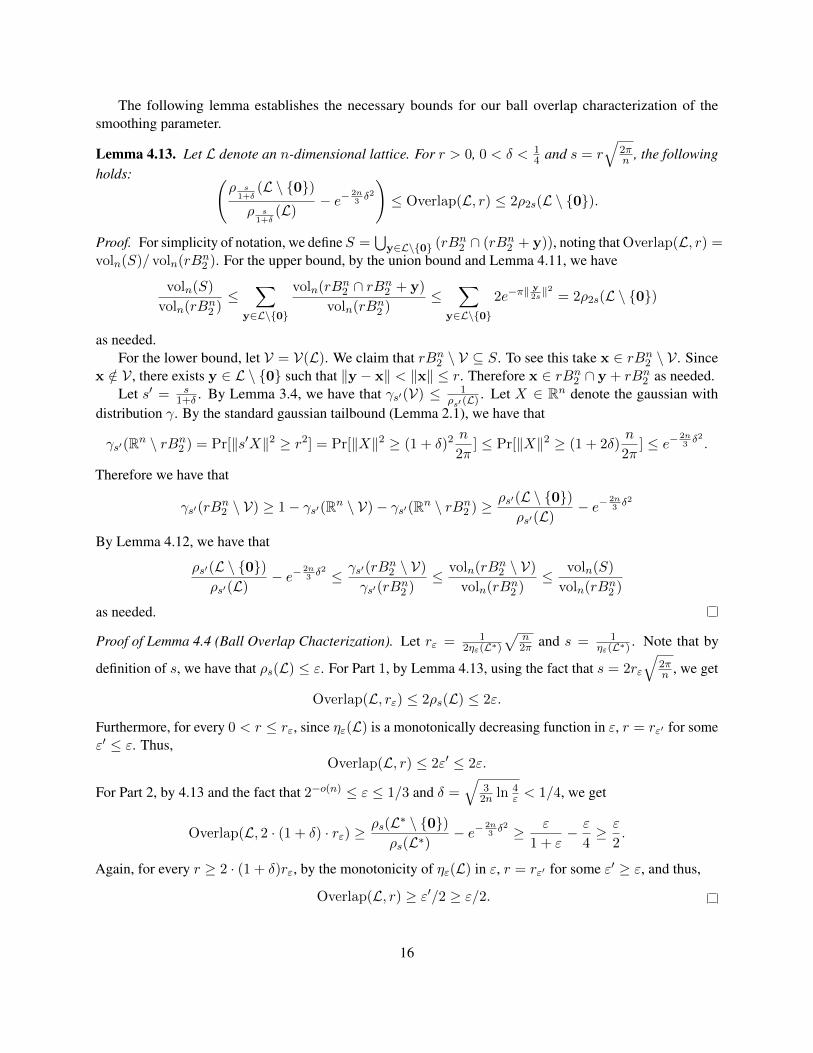
The following lemma establishes the necessary bounds for our ball overlap characterization of thesmoothing parameter.

Lemma 4.13. Let L denote an n-dimensional lattice. For r > 0, 0 < δ < 14 and s = r

√2πn , the following

holds: (ρ s

1+δ(L \ 0)

ρ s1+δ

(L)− e−

2n3δ2

)≤ Overlap(L, r) ≤ 2ρ2s(L \ 0).

Proof. For simplicity of notation, we define S =⋃

y∈L\0 (rBn2 ∩ (rBn

2 + y)), noting that Overlap(L, r) =voln(S)/ voln(rBn

2 ). For the upper bound, by the union bound and Lemma 4.11, we have

voln(S)

voln(rBn2 )≤

∑y∈L\0

voln(rBn2 ∩ rBn

2 + y)

voln(rBn2 )

≤∑

y∈L\0

2e−π‖y2s‖2 = 2ρ2s(L \ 0)

as needed.For the lower bound, let V = V(L). We claim that rBn

2 \ V ⊆ S. To see this take x ∈ rBn2 \ V . Since

x /∈ V , there exists y ∈ L \ 0 such that ‖y − x‖ < ‖x‖ ≤ r. Therefore x ∈ rBn2 ∩ y + rBn

2 as needed.Let s′ = s

1+δ . By Lemma 3.4, we have that γs′(V) ≤ 1ρs′ (L) . Let X ∈ Rn denote the gaussian with

distribution γ. By the standard gaussian tailbound (Lemma 2.1), we have that

γs′(Rn \ rBn2 ) = Pr[‖s′X‖2 ≥ r2] = Pr[‖X‖2 ≥ (1 + δ)2 n

2π] ≤ Pr[‖X‖2 ≥ (1 + 2δ)

n

2π] ≤ e−

2n3δ2.

Therefore we have that

γs′(rBn2 \ V) ≥ 1− γs′(Rn \ V)− γs′(Rn \ rBn

2 ) ≥ ρs′(L \ 0)ρs′(L)

− e−2n3δ2

By Lemma 4.12, we have that

ρs′(L \ 0)ρs′(L)

− e−2n3δ2 ≤ γs′(rB

n2 \ V)

γs′(rBn2 )

≤ voln(rBn2 \ V)

voln(rBn2 )

≤ voln(S)

voln(rBn2 )

as needed.

Proof of Lemma 4.4 (Ball Overlap Chacterization). Let rε = 12ηε(L∗)

√n2π and s = 1

ηε(L∗) . Note that by

definition of s, we have that ρs(L) ≤ ε. For Part 1, by Lemma 4.13, using the fact that s = 2rε

√2πn , we get

Overlap(L, rε) ≤ 2ρs(L) ≤ 2ε.

Furthermore, for every 0 < r ≤ rε, since ηε(L) is a monotonically decreasing function in ε, r = rε′ for someε′ ≤ ε. Thus,

Overlap(L, r) ≤ 2ε′ ≤ 2ε.

For Part 2, by 4.13 and the fact that 2−o(n) ≤ ε ≤ 1/3 and δ =√

32n ln 4

ε < 1/4, we get

Overlap(L, 2 · (1 + δ) · rε) ≥ρs(L∗ \ 0)ρs(L∗)

− e−2n3δ2 ≥ ε

1 + ε− ε

4≥ ε

2.

Again, for every r ≥ 2 · (1 + δ)rε, by the monotonicity of ηε(L) in ε, r = rε′ for some ε′ ≥ ε, and thus,

Overlap(L, r) ≥ ε′/2 ≥ ε/2.

16

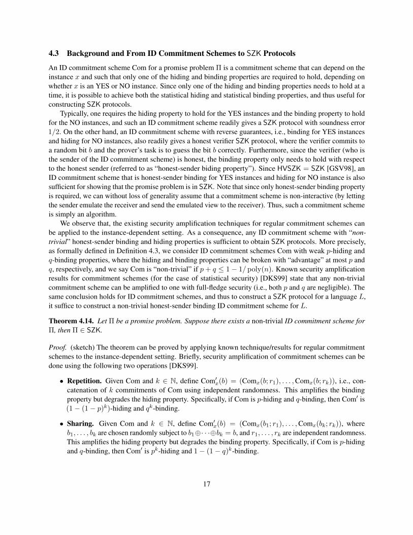
4.3 Background and From ID Commitment Schemes to SZK Protocols

An ID commitment scheme Com for a promise problem Π is a commitment scheme that can depend on theinstance x and such that only one of the hiding and binding properties are required to hold, depending onwhether x is an YES or NO instance. Since only one of the hiding and binding properties needs to hold at atime, it is possible to achieve both the statistical hiding and statistical binding properties, and thus useful forconstructing SZK protocols.

Typically, one requires the hiding property to hold for the YES instances and the binding property to holdfor the NO instances, and such an ID commitment scheme readily gives a SZK protocol with soundness error1/2. On the other hand, an ID commitment scheme with reverse guarantees, i.e., binding for YES instancesand hiding for NO instances, also readily gives a honest verifier SZK protocol, where the verifier commits toa random bit b and the prover’s task is to guess the bit b correctly. Furthermore, since the verifier (who isthe sender of the ID commitment scheme) is honest, the binding property only needs to hold with respectto the honest sender (referred to as “honest-sender biding property”). Since HVSZK = SZK [GSV98], anID commitment scheme that is honest-sender binding for YES instances and hiding for NO instance is alsosufficient for showing that the promise problem is in SZK. Note that since only honest-sender binding propertyis required, we can without loss of generality assume that a commitment scheme is non-interactive (by lettingthe sender emulate the receiver and send the emulated view to the receiver). Thus, such a commitment schemeis simply an algorithm.

We observe that, the existing security amplification techniques for regular commitment schemes canbe applied to the instance-dependent setting. As a consequence, any ID commitment scheme with “non-trivial” honest-sender binding and hiding properties is sufficient to obtain SZK protocols. More precisely,as formally defined in Definition 4.3, we consider ID commitment schemes Com with weak p-hiding andq-binding properties, where the hiding and binding properties can be broken with “advantage” at most p andq, respectively, and we say Com is “non-trivial” if p+ q ≤ 1− 1/poly(n). Known security amplificationresults for commitment schemes (for the case of statistical security) [DKS99] state that any non-trivialcommitment scheme can be amplified to one with full-fledge security (i.e., both p and q are negligible). Thesame conclusion holds for ID commitment schemes, and thus to construct a SZK protocol for a language L,it suffice to construct a non-trivial honest-sender binding ID commitment scheme for L.

Theorem 4.14. Let Π be a promise problem. Suppose there exists a non-trivial ID commitment scheme forΠ, then Π ∈ SZK.

Proof. (sketch) The theorem can be proved by applying known technique/results for regular commitmentschemes to the instance-dependent setting. Briefly, security amplification of commitment schemes can bedone using the following two operations [DKS99].

• Repetition. Given Com and k ∈ N, define Com′x(b) = (Comx(b; r1), . . . ,Comx(b; rk)), i.e., con-catenation of k commitments of Com using independent randomness. This amplifies the bindingproperty but degrades the hiding property. Specifically, if Com is p-hiding and q-binding, then Com′ is(1− (1− p)k)-hiding and qk-binding.

• Sharing. Given Com and k ∈ N, define Com′x(b) = (Comx(b1; r1), . . . ,Comx(bk; rk)), whereb1, . . . , bk are chosen randomly subject to b1⊕· · ·⊕bk = b, and r1, . . . , rk are independent randomness.This amplifies the hiding property but degrades the binding property. Specifically, if Com is p-hidingand q-binding, then Com′ is pk-hiding and 1− (1− q)k-binding.

17

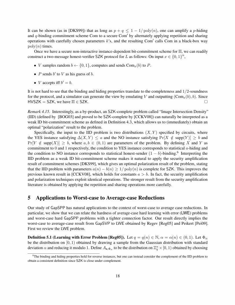
It can be shown (as in [DKS99]) that as long as p + q ≤ 1 − 1/ poly(n), one can amplify a p-hidingand q-binding commitment scheme Com to a secure Com′ by alternately applying repetition and sharingoperations with carefully chosen parameters k’s, and the resulting Com′ calls Com in a black-box waypoly(n) times.

Once we have a secure non-interactive instance-dependent bit-commitment scheme for Π, we can readilyconstruct a two-message honest-verifier SZK protocol for L as follows: On input x ∈ 0, 1n,

• V samples random b← 0, 1, computes and sends Comx(b) to P .

• P sends b′ to V as his guess of b.

• V accepts iff b′ = b.

It is not hard to see that the binding and hiding properties translate to the completeness and 1/2-soundnessfor the protocol, and a simulator can generate the view by emulating V and outputting (Comx(b), b). SinceHVSZK = SZK, we have Π ∈ SZK.

Remark 4.15. Interestingly, as a by-product, an SZK-complete problem called “Image Intersection Density”(IID) (defined by [BOG03] and proved to be SZK-complete by [CCKV08]) can naturally be interpreted as aweak ID bit-commitment scheme as defined in Definition 4.3, which allows us to (immediately) obtain anoptimal “polarization” result to the problem.

Specifically, the input to the IID problem is two distributions (X,Y ) specified by circuits, wherethe YES instance satisfying ∆(X,Y ) ≤ a and the NO instance satisfying Pr[X /∈ supp(Y )] ≥ b andPr[Y /∈ supp(X)] ≥ b, where a, b ∈ (0, 1) are parameters of the problem. By defining X and Y ascommitment to 0 and 1 respectively, the condition to YES instance corresponds to statistical a-hiding andthe condition to NO instance corresponds to statistical honest-sender (1 − b)-binding.6 Interpreting theIID problem as a weak ID bit-commitment scheme makes it natural to apply the security amplificationresult of commitment schemes [DKS99], which gives an optimal polarization result of the problem, statingthat the IID problem with parameters a(n) − b(n) ≥ 1/poly(n) is complete for SZK. This improves theprevious known result in [CCKV08], which holds for constants a > b. In fact, the security amplificationand polarization techniques exploit identical operations. The stronger result from the security amplificationliterature is obtained by applying the repetition and sharing operations more carefully.

5 Applications to Worst-case to Average-case Reductions

Our study of GapSPP has natural applications to the context of worst-case to average case reductions. Inparticular, we show that we can relate the hardness of average-case hard learning with error (LWE) problemsand worst-case hard GapSPP problems with a tighter connection factor. Our result directly implies theworst-case to average-case result from GapSVP to LWE obtained by Regev [Reg05] and Peikert [Pei09].First we review the LWE problem.

Definition 5.1 (Learning with Error Problem [Reg05]). Let q = q(n) ∈ N, α = α(n) ∈ (0, 1). Let Φα

be the distribution on [0, 1) obtained by drawing a sample from the Gaussian distribution with standarddeviation α and reducing it modulo 1. Define As,Φα to be the distribution on Znq × [0, 1) obtained by choosing

6The binding and hiding properties hold for reverse instances, but one can instead consider the complement of the IID problem toobtain a consistent definition since SZK is close under complement.

18

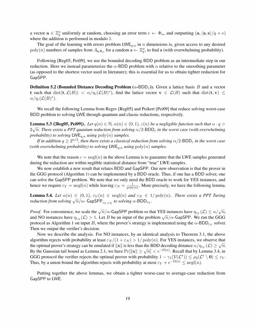
a vector a ∈ Znq uniformly at random, choosing an error term e ← Φα, and outputting (a, 〈a, s〉/q + e)where the addition is performed in modulo 1.

The goal of the learning with errors problem LWEq,α in n dimensions is, given access to any desiredpoly(n) numbers of samples from As,Φα for a random s← Znq , to find s (with overwhelming probability).

Following [Reg05, Pei09], we use the bounded decoding BDD problem as an intermediate step in ourreduction. Here we instead parameterize the α-BDD problem with α relative to the smoothing parameter(as opposed to the shortest vector used in literature); this is essential for us to obtain tighter reduction forGapSPP.

Definition 5.2 (Bounded Distance Decoding Problem (α-BDDε)). Given a lattice basis B and a vectort such that dist(t,L(B)) < α/ηε(L(B)∗), find the lattice vector v ∈ L(B) such that dist(t,v) ≤α/ηε(L(B)∗).

We recall the following Lemma from Regev [Reg05] and Peikert [Pei09] that reduce solving worst-caseBDD problem to solving LWE through quantum and classic reductions, respectively.

Lemma 5.3 ([Reg05, Pei09]). Let q(n) ∈ N, α(n) ∈ (0, 1), ε(n) be a negligible function such that α · q >2√n. There exists a PPT quantum reduction from solving α/2-BDDε in the worst case (with overwhelming

probability) to solving LWEq,α using poly(n) samples.If in addition q ≥ 2n/2, then there exists a classical reduction from solving α/2-BDDε in the worst case

(with overwhelming probability) to solving LWEq,α using poly(n) samples.

We note that the reason ε = negl(n) in the above Lemma is to guarantee that the LWE samples generatedduring the reduction are within neglible statistical distance from “true” LWE samples.

We now establish a new result that relates BDD and GapSPP. Our new observation is that the prover inthe GGG protocol (Algorithm 1) can be implemented by a BDD oracle. Thus, if one has a BDD solver, onecan solve the GapSPP problem. We note that we only need the BDD oracle to work for YES instances, andhence we require εY = negl(n) while leaving εN = 1

poly(n) . More precisely, we have the following lemma.

Lemma 5.4. Let α(n) ∈ (0, 1), εY (n) ∈ negl(n) and εN ∈ 1/poly(n). There exists a PPT Turingreduction from solving

√n/α- GapSPPεY ,εN to solving α-BDDεY .

Proof. For convenience, we scale the√n/α-GapSPP problem so that YES instances have ηεY (L) ≤ α/

√n,

and NO instances have ηεN (L) > 1. Let B be an input of the problem√n/α-GapSPP. We run the GGG

protocol as Algorithm 1 on input B, where the prover’s strategy is implemented using the α-BDDεY solver.Then we output the verifier’s decision.

Now we describe the analysis. For NO instances, by an identical analysis to Theorem 3.1, the abovealgorithm rejects with probability at least εN/(1 + εN ) > 1/ poly(n). For YES instances, we observe thatthe optimal prover’s strategy can be emulated if ‖x‖ is less than the BDD decoding distance α/ηεY (L) ≥

√n.

By the Gaussian tail bound as Lemma 2.1, we have Pr[‖x‖ ≥√n] < e−Ω(n). Recall that by Lemma 3.4, in

GGG protocol the verifier rejects the optimal prover with probability 1 − γ1(V(L∗)) ≤ ρ2(L∗ \ 0) ≤ εY .Thus, by a union bound the algorithm rejects with probability at most εY + e−Ω(n) ≤ negl(n).

Putting together the above lemmas, we obtain a tighter worse-case to average-case reduction fromGapSPP to LWE.

19

Theorem 5.5. Let q(n) ∈ N, α(n) ∈ (0, 1), εY (n) ∈ negl(n) and εN ∈ 1/ poly(n) such that α · q >2√n. There exists a PPT quantum reduction from solving 2

√n/α- GapSPPεY ,εN in the worst case (with

overwhelming probability) to solving LWEq,α using poly(n) samples.If in addition q ≥ 2n/2, then there exists a classical reduction from solving 2

√n/α- GapSPPεY ,εN in the

worst case (with overwhelming probability) to solving LWEq,α using poly(n) samples.

Remark 5.6. By using the following relation of shortest vectors and smoothing parameters by Micciancioand Regev [MR04]: √

log(1/ε)√πλ1(L∗)

≤ ηε(L) ≤√n

λ1(L∗)for ε ∈ [2−n, 1],

the above theorem implies that there exists a corresponding PPT quantum/classical reduction from (c· nα√

logn)-

GapSVP to LWEq,α for any constant c > 0.

6 Co-AM Protocol for GapSPP

In this section, we describe an co-AM protocol for GapSPP. Formally, we establish the following:

Theorem 6.1. For any α ≥ 1/poly(n) and εY , εN such that εN ≥ (1 + 1/ poly(n)) · εY , we have (1 +α)-GapSPPεY ,εN ∈ coAM.

By applying Corollary 2.5, we obtain the following upper bound on the complexity of γ-GapSPPε.

Corollary 6.2. For every ε : N→ (0, 1) such that ε(n) < 1− 1/ poly(n), we have (1 + o(1))-GapSPPε ∈coAM.

Our main tool is the classic set size lower bound protocol by Goldwasser and Sipser [GS86]. We use thisprotocol to show that the smoothing parameter should be at least as large as some quantity. To show thatη(L) is large, equivalently we are showing that the discrete Gaussian weights are large for the points in L∗inside the

√n ball7. (The Gaussian weights outside the ball becomes exponentially small.)

The set size lower bound protocol gives a very accurate approximation of lattice points inside the√n

ball, but its set size is not sufficient to approximate the Gaussian weights. The two points inside the ballcould have lengths that differ a lot, and thus their Gaussian weights differ even more. Our new observation isthat we can partition the

√n ball into different shells (con-centered at 0), and then use the set size protocol

to approximate the number of lattice points lying in each shell. Since every point in the same shell hasroughly the same length and thus Gaussian weight, we can approximate the total Gaussian weights in a shellaccording to the size. Thus, summing up the Gaussian weight of each shell, we are able to approximate theGaussian weights inside the

√n ball. Thus, we are able to show that the Gaussian weights inside the ball are

large, and thus η is large.First we describe the set size lower bound protocol:

Definition 6.3 (Set size lower bound protocol [GS86]). Let V be a probabilistic polynomial time verifier,and P be a (computationally unbounded) prover. Let S ⊆ 0, 1n be a set whose membership can beefficiently certified. The two parties hold common inputs 1n and K ∈ N.

We say 〈P,V〉 is a (1− γ)-approximation protocol of the set size |S| if the following conditions hold:

7Actually the radius needs to depend on the parameter εY . Here for simplicity we think εY as a constant.

20

• (Completeness) If |S| ≥ K, then V will always accept.

• (Soundness) If |S| < (1 − γ) · K, then V will accept with probability at most negl(n) for somenegligible function negl(·).

Now we recall the classic construction of the set size lower bound protocol:

Theorem 6.4 ([GS86]). For any set S ∈ 0, 1n whose membership can be efficiently certified, and anyγ = 1/ poly(n), there exists a public-coin, 2-round (1− γ)-approximation protocol of the set size |S|.

Moreover, for any k = poly(n), we can run the protocol k-times in parallel for k set-number pairs(Si,Ki)i∈[k], and the resulting protocol has perfect completeness and negligible soundness error. Heresoundness error means the probability that there exists some i∗ ∈ [k] such that |Si| ≤ (1 − γ) ·Ki but Vaccepts.

Proof of Theorem 6.1. To show the theorem, we first describe a coAM protocol 〈P,V〉 in the following.Note that the verifier in a coAM protocol must accept the NO instances and reject the YES instances of(1 + α)-GapSPPεY ,εN . For convenience, the YES or NO instances here are with respect to the GapSPPproblem, so the completeness means the verifier accepts any NO instance, and the soundness means he rejectsany YES instance.

Let B be an n-dimensional basis of a lattice L as input to the prover and verifier, satisfying eitherηεN (L) ≥ (1 + α) (NO instance) or ηεY (L) ≤ 1 (YES instance), where α ≥ 1/ poly(n), εN ≥ (1 +1/ poly(n)) · εY . The prover and the verifier agree on the following parameters:

Parameters. Let R = n · (1 + log(1/εY )), 1 − β = 2εYεY +εN

, and let T = d log√R

log(1+α)e. We know forα ≥ 1/ poly(n) being noticeable, we have T bounded by some polynomial, i.e. T ≤ poly(n). Then

we define spaces S0def= v ∈ L∗ : 0 < ‖v‖ ≤ 1, and Si

def=v ∈ L∗ : (1 + α)i−1 < ‖v‖ ≤ (1 + α)i

, for

i ∈ [T ]. Pictorially, these Si’s form a partition of space inside the region of√RBn

2 . Each Si is a shell thatcontains lattice points from length (1 + α)i−1 to (1 + α)i.

Then 〈P,V〉 does the following:

• P sends K0,K1,K2, . . .KT ∈ N as claims of the sizes of S0, S1, S2, . . . , ST .

• Then for each pair (Si,Ki), P and V run the (1 − β)-approximation protocol as its subroutine.These T approximation protocols are run in parallel. Note that 2εY

εY +εN≤ 1 − 1/ poly(n) since

εN ≥ (1 + 1/ poly(n)) · εY . Thus, 1− β ≤ 1− 1/poly(n), which is within the range of parametersof the set size lower bound.

• In the end, V accepts if and only if all the approximation subprotocols are accepted, and∑

0≤i≤T Ki ·e−π(1+α)2i ≥ (εY + εN )/2.

It is easy to see that the verifier can be implemented in probabilistic polynomial time. It remains to showthe completeness and soundness. We show them by the following two claims:

Claim 6.5. If B is a NO instance, V will always accept the honest prover’s strategy.

21

Proof. Let K0,K1, . . . ,KT be the values of the set sizes S0, S1, . . . , ST , as the honest prover will alwayssend the correct values. From the promise of NO instances, we know ηεN (L) ≥ (1 + α), which implies

qdef=

∑v∈L∗\0

e−π(1+α)2‖v‖2 ≥ εN .

By rearranging the order of summation, we have

q =∑

0≤i≤T

∑v∈Si

e−π(1+α)2‖v‖2 +∑

v∈L∗\(√R·Bn2 )

e−π(1+α)2‖v‖2

≤∑

0≤i≤T

∑v∈Si

e−π(1+α)2‖v‖2 + 2−n · εY

≤∑

0≤i≤TKi · e−π(1+α)2i

+ 2−n · εY .

The first equality comes from the rearrangement; the second line is a tail bound inequality by Lemma 2.1by plugging suitable parameters; the last inequality is by the fact that v ∈ Si implies ‖v‖ ≥ (1 + α)i−1 fori ∈ [T ].

Then we have ∑0≤i≤T

Ki · e−π(1+α)2i ≥ εN − 2−n · εY ≥ (εY + εN )/2,

for all sufficiently large n’s. This follows by the fact that εN ≥ (1 + 1/ poly(n)) · εY , and a straightforwardexamination. Thus, the verifier will always accept.

Claim 6.6. If B is a YES instance, then no prover can convince the verifier with probability better than anegligible quantity.

Proof. From the promise of YES instances, we know ηεY (L) ≤ 1, which implies

qdef=

∑v∈L∗\0

e−π‖v‖2 ≤ εY .

Similarly, we rearrange the order of summation and get

q =∑

0≤i≤T

∑v∈Si

e−π‖v‖2

+∑

v∈L∗\(√R·Bn2 )

e−π‖v‖2

≥∑

0≤i≤T

∑v∈Si

e−π‖v‖2

≥∑

0≤i≤T|Si| · e−π(1+α)2i

.

Suppose the prover sends someK0,K1 . . .KT such that∑

0≤i≤T Ki ·e−π(1+α)2i ≥ (εY +εN )/2, it mustbe the case that ∃i∗ ∈ [T ] such that εY

(εY +εN )/2Ki = (1−β) ·Ki ≥ |Si| from a simple counting argument. Bythe soundness of the (1−β)-approximation protocol, the verifier will catch this with probability (1−negl(n)).Hence the verifier accepts a YES instance with only negligible probability.

Together with the two claims, the proof of the theorem is complete.

22

7 Deterministic Algorithm for Smoothing Parameter

In this section we show that (1 + o(1))-GapSPP can be solved deterministically in time 2O(n). In particularwe are able to show the following theorem.

To show the theorem, use are going to establish the following lemma.

Theorem 7.1. For any εY , εN : N → [0, 1] such that εN (n) − εY (n) ≥ 1/2−2n, 1-GapSPPεY ,εN ∈DTIME (2O(n)).

Together with Corollary 2.5, we are able to obtain the following corollary.

Corollary 7.2. For any ε : N→ [0, 1] and ε(n) ≥ 2−n, the problem (1+o(1))-GapSPPε ∈ DTIME (2O(n)).

We will crucially use the following lattice point enumeration algorithm. The algorithm is a slight tweakof closest vector problem algorithm of Micciancio and Voulgaris [MV10], which was first used in [DPV11]to solve the shortest vector problem in general norms.

Proposition 7.3 ([MV10, DPV11], Algorithm Ball-Enum). There is an algorithm Ball-Enum that given aradius r > 0, a basis B of an n-dimensional lattice L, and t ∈ Rn, lazily enumerates the set L ∩ (rBn

2 + t)in deterministic time 2O(n) · (|L ∩ (t+ rBn

2 )|+ 1) using at most 2O(n) space.

Now we are ready to prove Theorem 7.1 using the above theorem.

Proof. Let B be an n-dimensional basis of a lattice L satisfying either ηεY ≤ 1 or ηεN ≥ 1, where εY , εNare parameters that the conditions in the theorem hold. Now we are going to describe an algorithm A oninput B that distinguishes the two cases.

A runs the enumeration algorithm with the parameters t = 0, r =√n to enumerate all points in

L∗ ∩√n ·Bn

2 . If A has already found eπ·n · εN points from the enumeration algorithm, A terminates andrejects immediately. This is because∑

v∈L∗\0

e−π‖v‖2 ≥

∑v∈(L∗\0)∩

√n·Bn2

e−π‖v‖2 ≥ (eπn · εN ) · e−πn = εN ,

which already implies the case of no instances.Otherwise A computes u =

∑v∈(L∗\0)∩

√n·Bn2

e−π‖v‖2. A accepts if u ≤ (εY + εN )/2, and otherwise

rejects. The analysis of its completeness and soundness is very similar to that of Theorem 6.1, so we do notrestate it here. It is not hard to see that this can be done in time 2O(n) · eπn · εN = 2O(n).

Acknowledgments

We thank Oded Regev for helpful discussions. We also thank the anonymous reviewers for helpful suggestions.

References

[Ajt96] M. Ajtai. Generating hard instances of lattice problems. Quaderni di Matematica, 13:1–32,2004. Preliminary version in STOC 1996.

23

[AR04] D. Aharonov and O. Regev. Lattice problems in NP ∩ coNP. J. ACM, 52(5):749–765, 2005.Preliminary version in FOCS 2004.

[Bal97] K. M. Ball. An elementary introduction to modern convex geometry. In S. Levy (Ed.), Flavors ofGeometry, Number 31 in MSRI Publications, pages 1–58, 1997.

[Ban93] W. Banaszczyk. New bounds in some transference theorems in the geometry of numbers.Mathematische Annalen, 296(4):625–635, 1993.

[Ban95] W. Banaszczyk. Inequalites for convex bodies and polar reciprocal lattices in Rn. Discrete &Computational Geometry, 13:217–231, 1995.

[Ban96] W. Banaszczyk. Inequalities for convex bodies and polar reciprocal lattices in Rn II: Applicationof k-convexity. Discrete and Computational Geometry, 16:305–311, 1996. ISSN 0179-5376.

[BHZ87] R. B. Boppana, J. Hastad, and S. Zachos. Does co-NP have short interactive proofs? Inf. Process.Lett., 25(2):127–132, 1987.

[BOG03] M. Ben-Or and D. Gutfreund. Trading help for interaction in statistical zero-knowledge proofs.J. Cryptology, 16(2):95–116, 2003.

[BV11] Z. Brakerski and V. Vaikuntanathan. Efficient fully homomorphic encryption from (standard)LWE. In FOCS, pages 97–106. 2011.

[CCKV08] A. Chailloux, D. F. Ciocan, I. Kerenidis, and S. P. Vadhan. Interactive and noninteractive zeroknowledge are equivalent in the help model. In TCC, pages 501–534. 2008.

[CH11] H. Cohn and N. Heninger. Ideal forms of Coppersmith’s theorem and Guruswami-Sudan listdecoding. In ICS, pages 298–308. 2011.

[CHKP10] D. Cash, D. Hofheinz, E. Kiltz, and C. Peikert. Bonsai trees, or how to delegate a lattice basis.In EUROCRYPT, pages 523–552. 2010.

[Cop97] D. Coppersmith. Small solutions to polynomial equations, and low exponent RSA vulnerabilities.J. Cryptology, 10(4):233–260, 1997.

[DKS99] I. Damgard, J. Kilian, and L. Salvail. On the (im)possibility of basing oblivious transfer and bitcommitment on weakened security assumptions. In EUROCRYPT, pages 56–73. 1999.

[DPV11] D. Dadush, C. Peikert, and S. Vempala. Enumerative lattice algorithms in any norm via M-ellipsoid coverings. In FOCS, pages 580–589. 2011.

[Gen09] C. Gentry. Fully homomorphic encryption using ideal lattices. In STOC, pages 169–178. 2009.

[Gen10] C. Gentry. Toward basing fully homomorphic encryption on worst-case hardness. In CRYPTO,pages 116–137. 2010.

[GG98] O. Goldreich and S. Goldwasser. On the limits of nonapproximability of lattice problems. J.Comput. Syst. Sci., 60(3):540–563, 2000. Preliminary version in STOC 1998.

[GMR04] V. Guruswami, D. Micciancio, and O. Regev. The complexity of the covering radius problem.Computational Complexity, 14(2):90–121, 2005. Preliminary version in CCC 2004.

24

[GPV08] C. Gentry, C. Peikert, and V. Vaikuntanathan. Trapdoors for hard lattices and new cryptographicconstructions. In STOC, pages 197–206. 2008.

[GS86] S. Goldwasser and M. Sipser. Private coins versus public coins in interactive proof systems. InSTOC, pages 59–68. 1986.

[GS88] J. Grollmann and A. L. Selman. Complexity measures for public-key cryptosystems. SIAM J.Comput., 17(2):309–335, 1988.

[GSV98] O. Goldreich, A. Sahai, and S. P. Vadhan. Honest-verifier statistical zero-knowledge equalsgeneral statistical zero-knowledge. In STOC, pages 399–408. 1998.

[IOS97] T. Itoh, Y. Ohta, and H. Shizuya. A language-dependent cryptographic primitive. J. Cryptology,10(1):37–50, 1997.

[LLL82] A. K. Lenstra, H. W. Lenstra, Jr., and L. Lovasz. Factoring polynomials with rational coefficients.Mathematische Annalen, 261(4):515–534, December 1982.

[MR04] D. Micciancio and O. Regev. Worst-case to average-case reductions based on Gaussian measures.SIAM J. Comput., 37(1):267–302, 2007. Preliminary version in FOCS 2004.

[MV03] D. Micciancio and S. P. Vadhan. Statistical zero-knowledge proofs with efficient provers: Latticeproblems and more. In CRYPTO, pages 282–298. 2003.

[MV10] D. Micciancio and P. Voulgaris. A deterministic single exponential time algorithm for mostlattice problems based on Voronoi cell computations. In STOC, pages 351–358. 2010.

[Pei07] C. Peikert. Limits on the hardness of lattice problems in `p norms. Computational Complexity,17(2):300–351, May 2008. Preliminary version in CCC 2007.

[Pei09] C. Peikert. Public-key cryptosystems from the worst-case shortest vector problem. In STOC,pages 333–342. 2009.

[Pei10] C. Peikert. An efficient and parallel Gaussian sampler for lattices. In CRYPTO, pages 80–97.2010.

[PW08] C. Peikert and B. Waters. Lossy trapdoor functions and their applications. In STOC, pages187–196. 2008.

[Reg03] O. Regev. New lattice-based cryptographic constructions. J. ACM, 51(6):899–942, 2004.Preliminary version in STOC 2003.

[Reg05] O. Regev. On lattices, learning with errors, random linear codes, and cryptography. J. ACM,56(6):1–40, 2009. Preliminary version in STOC 2005.

[SV03] A. Sahai and S. P. Vadhan. A complete problem for statistical zero knowledge. J. ACM,50(2):196–249, 2003.

25