On the application and interpretation of Keeling plots in ... · paleo extension of the two...

Biogeosciences, 3, 539–556, 2006www.biogeosciences.net/3/539/2006/© Author(s) 2006. This work is licensedunder a Creative Commons License.

Biogeosciences

On the application and interpretation of Keeling plots in paleoclimate research – deciphering δ13C of atmospheric CO2 measuredin ice coresP. Kohler1, H. Fischer1, J. Schmitt1, and G. Munhoven2

1Alfred Wegener Institute, Helmholtz Center for Polar and Marine Research, P.O. Box 12 01 61, 27515 Bremerhaven,Germany2Laboratoire de Physique Atmospherique et Planetaire, Institut d’Astrophysique et de Geophysique, Universite de Liege, 17avenue du Six-Aout, B–4000 Liege, Belgium

Received: 21 February 2006 – Published in Biogeosciences Discuss.: 14 June 2006Revised: 9 November 2006 – Accepted: 10 November 2006 – Published: 15 November 2006

Abstract. The Keeling plot analysis is an interpretationmethod widely used in terrestrial carbon cycle research toquantify exchange processes of carbon between terrestrialreservoirs and the atmosphere. Here, we analyse measureddata sets and artificial time series of the partial pressure of at-mospheric carbon dioxide (pCO2) and of δ13C of CO2 overindustrial and glacial/interglacial time scales and investigateto what extent the Keeling plot methodology can be appliedto longer time scales. The artificial time series are simula-tion results of the global carbon cycle box model BICYCLE.The signals recorded in ice cores caused by abrupt terrestrialcarbon uptake or release loose information due to air mix-ing in the firn before bubble enclosure and limited samplingfrequency. Carbon uptake by the ocean cannot longer be ne-glected for less abrupt changes as occurring during glacialcycles. We introduce an equation for the calculation of long-term changes in the isotopic signature of atmospheric CO2caused by an injection of terrestrial carbon to the atmosphere,in which the ocean is introduced as third reservoir. This is apaleo extension of the two reservoir mass balance equationsof the Keeling plot approach. It gives an explanation for thebias between the isotopic signature of the terrestrial releaseand the signature deduced with the Keeling plot approach forlong-term processes, in which the oceanic reservoir cannotbe neglected. These deduced isotopic signatures are similar(−8.6‰) for steady state analyses of long-term changes inthe terrestrial and marine biosphere which both perturb theatmospheric carbon reservoir. They are more positive thanthe δ13C signals of the sources, e.g. the terrestrial carbonpools themselves (∼ −25‰). A distinction of specific pro-cesses acting on the global carbon cycle from the Keeling

Correspondence to: P. Kohler([email protected])

plot approach is not straightforward. In general, processesrelated to biogenic fixation or release of carbon have lowery-intercepts in the Keeling plot than changes in physical pro-cesses, however in many case they are indistinguishable (e.g.ocean circulation from biogenic carbon fixation).

1 Introduction

In carbon cycle research information on the origin of fluxesbetween different reservoirs as contained in the ratio of thestable carbon isotopes 13C/12C has become more and moreimportant in the past decades. Differences in physical prop-erties of atoms and molecules containing different isotopesof an element lead to isotopic fractionation during mostphysico-chemical processes. Isotopic ratios therefore storeinformation about ongoing or past processes.

Prominent examples of processes during which isotopicfractionation occurs in our context of global carbon cycle re-search are gas exchange between surface ocean and atmo-sphere or photosynthetic production in both the marine andthe terrestrial biosphere. Here, the carbon reservoir whichincludes the end members of a carbon flux associated with agiven process is in general depleted in the heavier isotope.This is expressed with the fractionation ε of the process,which depends on various environmental parameters such astemperature or the biological species (see Zeebe and Wolf-Gladrow (2001) for more basic information on carbon iso-topes in seawater).

Published by Copernicus GmbH on behalf of the European Geosciences Union.

540 P. Kohler et al.: Deciphering δ13C of atmospheric CO2 measured in ice cores

The isotopic composition of a reservoir is usually ex-pressed in per mil (‰) in the so-called “δ-notation” as therelative deviation from the isotope ratio of a defined standard(VPDP in the case of δ13C):

δ13C sample =

13C12C sample

13C12C standard

− 1

× 103. (1)

The fractionation ε (in ‰) between carbon in sample A andin sample B (e.g. before and after some fractionation step) isrelated to the δ values by

ε(A−B) =δA

− δB

1 + δB/103 . (2)

During photosynthesis the carbon taken up by marine pri-mary producers is typically depleted by −16 to −20‰. Onland, the type of metabolism determines the fractionationduring terrestrial photosynthesis. C3 plants exhibit a higherdiscrimination against the heavy isotope (ε=−15 to −23‰)than plants with C4 metabolism (ε=−2 to −8‰) (Mook,1986).

One prominent interpretation technique of carbon ex-change between the atmosphere and other reservoirs,e.g. used in carbon flux studies in terrestrial ecosystems,is plotting the δ13C signature of CO2 as a function ofthe inverse of the atmospheric carbon dioxide mixing ratio(δ13C=f (1/CO2)). In doing so, the intercept of a linear re-gression with the y-axis can under certain conditions be un-derstood as the isotopic signature of the flux, which alters thecontent of carbon in the atmospheric reservoir. This approachis called “Keeling plot” after the very first usage by CharlesD. Keeling about 50 years ago (Keeling, 1958, 1961). Keel-ing plots are widely used for data interpretation in terrestrialcarbon research, however, their application is based on somefundamental assumptions (see review of Pataki et al., 2003).

Keeling plots have also been used in paleo climate re-search in the past years (e.g. Smith et al., 1999; Fischer et al.,2003). However, one of the fundamental limitations of theKeeling plot approach, which is its restriction to fast ex-change processes, has not been taken into account adequatelyin these studies. Therefore, the aim of this paper is to em-phasise what can be learnt from Keeling plots, if applied onslow, but global processes acting on glacial/interglacial timescales, and to discuss their limitations. We emphasise whatkind of information can be gained from deciphering the δ13Csignal measured in ice cores. For this purpose we first extentthe Keeling plot approach to a three reservoir system and thenanalyse measured data sets and artificial time series, the latterproduced by a global carbon cycle box model. The advantageof the analysis of model output is, that we know which pro-cesses were active and thus responsible for the changes in theglobal carbon cycle.

2 The original Keeling plot

The Keeling plot approach is based upon mass conservationconsiderations during the exchange of carbon between tworeservoirs. Let Cnew be the mass of carbon after the additionof carbon with mass Cadd to an reservoir with an initial massCold.

Cnew = Cold + Cadd (3)

We denote by δ13Cx the carbon isotopic signature of the Ccomponent x, conservation of mass requires that

Cnewδ13Cnew = Cold · δ13Cold + Cadd · δ13Cadd. (4)

By combining Eqs. (3) and (4) we obtain a relationship be-tween δ13Cnew and Cnew:

δ13Cnew = (δ13Cold − δ13Cadd)Cold

Cnew+ δ13Cadd. (5)

Thus, the y-intercept y0 of the linear regression function ofEq. (5), which describes δ13Cnew as a function of the inverseof the carbon content (1/Cnew), gives us the isotopic signatureδ13Cadd of the carbon added to the reservoir.

There are two basic assumptions underlying the Keelingplot method: (1) The system consists of only two reservoirs.(2) The isotopic ratio of the carbon in the added reservoirdoes not change during the time of observation. Both as-sumptions are only rarely fulfilled. Furthermore, there arearguments about which linear regression model should beused if one assumes measurement errors in both variables(for details see Pataki et al., 2003). The methodological as-pects concerning the choice of a regression model are not thesubject of our investigations here.

The Keeling plot approach was used in the past to inter-pret various different sub-systems of the global carbon cycle.Keeling (1958, 1961) first used it to identify the contribu-tion of terrestrial plants to the background isotopic ratio ofCO2 in a rural area near the Pacific coast of North Amer-ica. Later, the contribution of the terrestrial biosphere in theseasonal cycle of CO2 over Switzerland (Friedli et al., 1986;Sturm et al., 2005) and Eurasia (Levin et al., 2002) was in-vestigated with the Keeling plot. The approach was widelyused in terrestrial ecosystem research to identify respirationfluxes (e.g. Flanagan and Ehleringer, 1998; Yakir and Stern-berg, 2000; Bowling et al., 2001; Pataki et al., 2003; Hem-ming et al., 2005). It was used in paleo climate researchwithin the last years to disentangle the processes explainingthe subtle changes in CO2 during the relatively stable LastGlacial Maximum (LGM) and the Holocene as well as theapproximately 80 ppmv increase from the LGM to the EarlyHolocene (Smith et al., 1999; Fischer et al., 2003).

Biogeosciences, 3, 539–556, 2006 www.biogeosciences.net/3/539/2006/

P. Kohler et al.: Deciphering δ13C of atmospheric CO2 measured in ice cores 541

16 P. Kohler et al.: Decipheringδ13C of atmospheric CO2 measured in ice cores

200

250

300

350

CO

2[p

pmv]

13CCO2

A

TD

30 1Time [kyr BP]

LD

1000 2000Time [yr AD]

2000

PB

1980 2000Time [yr AD]

-8.5

-8.0

-7.5

-7.0

-6.5

-6.0

13C

[o / oo]

0.003 0.004 0.0051/CO2 [1/ppmv]

-8.5

-8.0

-7.5

-7.0

-6.5

-6.0300 250 200

CO2 [ppmv]

...........................

...................................................

..............

...................................

....................................

.......................

..

.

........

......................................

...........................

............................................................................................................

....................................................

........

......................................................

. Point Barrow (PB), detrended

. Point Barrow (PB), originalLaw Dome (LD)Taylor Dome (TD) LGMTaylor Dome (TD) GIGTaylor Dome (TD) HOL

TD HOL: y0 = -9.5o/oo, r2 = 40%TD GIG: y0 = -5.8o/oo, r2 = 34%TD LGM: y0 = -9.5o/oo, r2 = 48%LD ANT: y0 = -13.1o/oo, r2 = 96%PB ORG: y0 = -16.7o/oo, r2 = 68%PB DET: y0 = -25.3o/oo, r2 = 96%

B

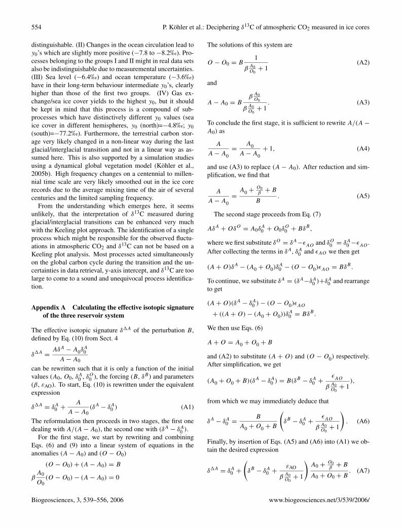
Fig. 1. A compilation of data from Point Barrow (PB), the Law Dome (LD), and theTaylor Dome (TD) ice cores (A: CO2, δ13C; B: Keelingplot). Monthly resolved data (1982−2002) from Point Barrow (Keeling and Whorf, 2005; Keeling et al., 2005). Only times where datain both CO2 andδ13C were available are considered here. For the Keeling plot approach theoriginal data (PB ORG) and detrended timeseries (PB DET) are plotted and analysed. Data from firn and ice at Law Dome cover the last millenium (Francey et al., 1999; Trudingeret al., 1999) which includes the anthropogenic rise in CO2 (LD ANT). Data from the Taylor Dome ice core of the last 30 kyr include theglacial/interglacial transition during Termination I (Smith et al., 1999) with the age model of Brook et al. (2000). Taylor Dome data are splitinto the Holocene (TD HOL), the glacial/interglacial transition (TD GIG), and the LGM (TD LGM).

Biogeosciences, 0000, 0001–24, 2006 www.biogeosciences.net/bg/0000/0001/

Fig. 1. A compilation of data from Point Barrow (PB), the Law Dome (LD), and the Taylor Dome (TD) ice cores ((a): CO2, δ13C; (b):Keeling plot). Monthly resolved data (1982−2002) from Point Barrow (Keeling and Whorf, 2005; Keeling et al., 2005). Only times wheredata in both CO2 and δ13C were available are considered here. For the Keeling plot approach the original data (PB ORG) and detrendedtime series (PB DET) are plotted and analysed. Data from firn and ice at Law Dome cover the last millenium (Francey et al., 1999; Trudingeret al., 1999) which includes the anthropogenic rise in CO2 (LD ANT). Data from the Taylor Dome ice core of the last 30 kyr include theglacial/interglacial transition during Termination I (Smith et al., 1999) with the age model of Brook et al. (2000). Taylor Dome data are splitinto the Holocene (TD HOL), the glacial/interglacial transition (TD GIG), and the LGM (TD LGM).

3 Global CO2 and δ13C time series of different temporalresolution

Fischer et al. (2003) used Keeling plots to analyse theseasonal amplitudes of CO2 and δ13C during the pastfew decades, the anthropogenic rise in CO2 and the con-comitant δ13C decrease since 1750 AD, as well as theirglacial/interglacial variations. As illustrated in Fig. 1, thesethree data sets which cover three completely different tem-poral scales exhibit significantly different behaviour.

As an example we take the seasonality of the atmosphericcarbon records at Point Barrow, Alaska, covering the periodfrom 1982 to 2002 AD (Keeling and Whorf, 2005; Keelinget al., 2005) where the seasonal cycle in CO2 and δ13C ismost pronounced. For the interpretation of this data set, thetime series need to be detrended to separate the seasonalityfrom the simultaneously occurring anthropogenic long-termtrend. Annual variations are then analysed as perturbationsfrom the mean values of the first year of the measurements.

For the anthropogenic variation during the last millenniumwe use the data measured in air enclosures in the Law Domeice core (Francey et al., 1999; Trudinger et al., 1999). Thecomponent Cadd in Eqs. (3)–(5) reflects the exchange of car-bon of an external reservoir with the atmospheric reservoir.The Point Barrow and Law Dome data can be approximatedconsistently with the typical Keeling plot linear regressionfunction (r2

=96% in both). The y-axis intercept y0 increasesfrom the seasonal effects (−25‰) to the anthropogenic im-pact (−13‰) with the mixed signal of the undetrended dataat Point Barrow in-between (−17‰) (Fig. 1b). This increase

is explained by a larger oceanic carbon uptake and a smallerairborne fraction of any atmospheric disturbance in CO2 inthe longer time series from the Law Dome ice core (Fischeret al., 2003).

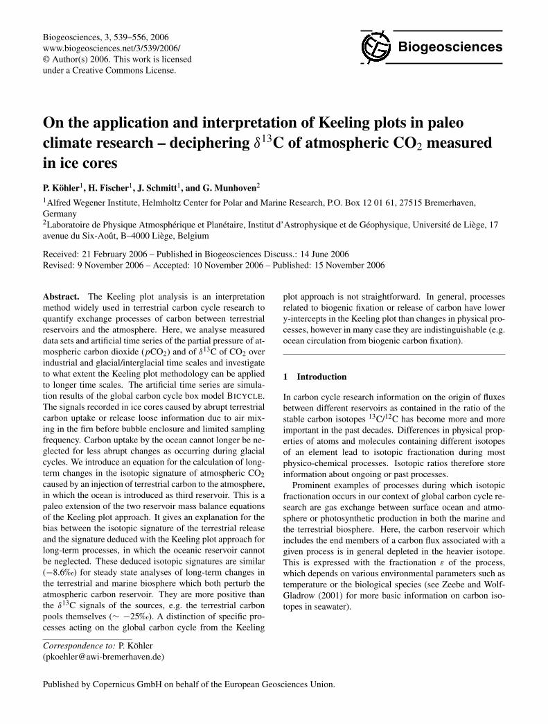
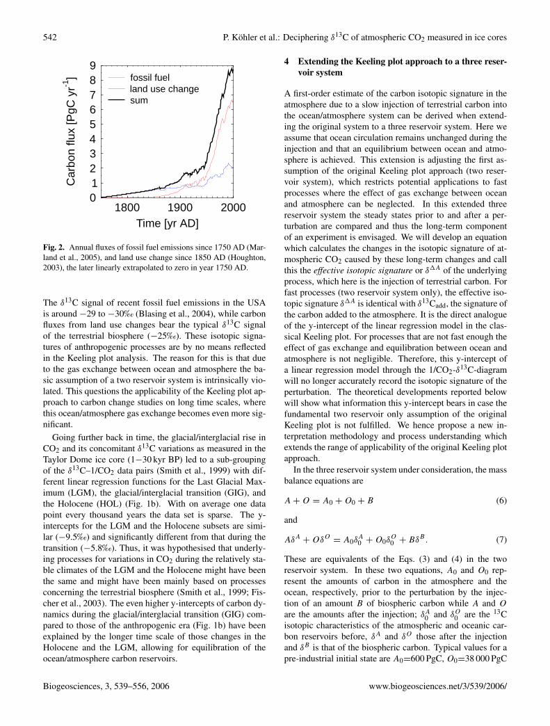
These two examples based on measured data sets are al-ready beyond the scope of Keeling’s original idea as they areno longer based on a two reservoir system and highlight thelimitations of this approach. While the y-intercept of the de-trended data at Point Barrow is consistent with the expectedvalue, the intercept found in the anthropogenic rise in LawDome does not record the δ13C signal of the carbon releasedby anthropogenic activity to the atmosphere. The seasonalamplitude at Point Barrow can be explained with the season-ality of the terrestrial biosphere. Vegetation grows mainly inthe northern hemisphere, and thus CO2 minima occur dur-ing maximum photosynthetic carbon uptake by plants duringnorthern summer. The seasonal fluctuation in CO2 shouldtherefore bear a δ13C signal of the order of −25‰ whichwould account for fractionation during terrestrial photosyn-thesis (Scholze et al., 2003). This δ13C signal of the seasonalcycle is seen in the detrended Point Barrow data in agree-ment with other studies (e.g. Levin et al., 2002). The riseseen in the Law Dome data set is the result of the combina-tion of anthropogenic activities (fossil fuel emissions (Mar-land et al., 2005) and land use changes (Houghton, 2003),Fig. 2), terrestrial carbon sinks due to CO2 fertilisation (Plat-tner et al., 2002), all from which the ocean carbon uptakeduring that time has to be subtracted. Without carbon uptakeby the ocean and the terrestrial reservoirs this would haveled to a rise in atmospheric CO2 by more than 200 ppmv.

www.biogeosciences.net/3/539/2006/ Biogeosciences, 3, 539–556, 2006


P. Kohler et al.: Decipheringδ13C of atmospheric CO2 measured in ice cores 17

1800 1900 2000Time [yr AD]

0123456789

Car

bon

flux

[PgC

yr-1

]

sumland use changefossil fuel

Fig. 2. Annual fluxes of fossil fuel emissions since 1750 AD (Marland et al.,2005), and land use change since 1850 AD (Houghton, 2003),the later linearly extrapolated to zero in year 1750 AD.

www.biogeosciences.net/bg/0000/0001/ Biogeosciences, 0000, 0001–24, 2006

Fig. 2. Annual fluxes of fossil fuel emissions since 1750 AD (Mar-land et al., 2005), and land use change since 1850 AD (Houghton,2003), the later linearly extrapolated to zero in year 1750 AD.

The δ13C signal of recent fossil fuel emissions in the USAis around −29 to −30‰ (Blasing et al., 2004), while carbonfluxes from land use changes bear the typical δ13C signalof the terrestrial biosphere (−25‰). These isotopic signa-tures of anthropogenic processes are by no means reflectedin the Keeling plot analysis. The reason for this is that dueto the gas exchange between ocean and atmosphere the ba-sic assumption of a two reservoir system is intrinsically vio-lated. This questions the applicability of the Keeling plot ap-proach to carbon change studies on long time scales, wherethis ocean/atmosphere gas exchange becomes even more sig-nificant.

Going further back in time, the glacial/interglacial rise inCO2 and its concomitant δ13C variations as measured in theTaylor Dome ice core (1−30 kyr BP) led to a sub-groupingof the δ13C–1/CO2 data pairs (Smith et al., 1999) with dif-ferent linear regression functions for the Last Glacial Max-imum (LGM), the glacial/interglacial transition (GIG), andthe Holocene (HOL) (Fig. 1b). With on average one datapoint every thousand years the data set is sparse. The y-intercepts for the LGM and the Holocene subsets are simi-lar (−9.5‰) and significantly different from that during thetransition (−5.8‰). Thus, it was hypothesised that underly-ing processes for variations in CO2 during the relatively sta-ble climates of the LGM and the Holocene might have beenthe same and might have been mainly based on processesconcerning the terrestrial biosphere (Smith et al., 1999; Fis-cher et al., 2003). The even higher y-intercepts of carbon dy-namics during the glacial/interglacial transition (GIG) com-pared to those of the anthropogenic era (Fig. 1b) have beenexplained by the longer time scale of those changes in theHolocene and the LGM, allowing for equilibration of theocean/atmosphere carbon reservoirs.

4 Extending the Keeling plot approach to a three reser-voir system

A first-order estimate of the carbon isotopic signature in theatmosphere due to a slow injection of terrestrial carbon intothe ocean/atmosphere system can be derived when extend-ing the original system to a three reservoir system. Here weassume that ocean circulation remains unchanged during theinjection and that an equilibrium between ocean and atmo-sphere is achieved. This extension is adjusting the first as-sumption of the original Keeling plot approach (two reser-voir system), which restricts potential applications to fastprocesses where the effect of gas exchange between oceanand atmosphere can be neglected. In this extended threereservoir system the steady states prior to and after a per-turbation are compared and thus the long-term componentof an experiment is envisaged. We will develop an equationwhich calculates the changes in the isotopic signature of at-mospheric CO2 caused by these long-term changes and callthis the effective isotopic signature or δ1A of the underlyingprocess, which here is the injection of terrestrial carbon. Forfast processes (two reservoir system only), the effective iso-topic signature δ1A is identical with δ13Cadd, the signature ofthe carbon added to the atmosphere. It is the direct analogueof the y-intercept of the linear regression model in the clas-sical Keeling plot. For processes that are not fast enough theeffect of gas exchange and equilibration between ocean andatmosphere is not negligible. Therefore, this y-intercept ofa linear regression model through the 1/CO2-δ13C-diagramwill no longer accurately record the isotopic signature of theperturbation. The theoretical developments reported belowwill show what information this y-intercept bears in case thefundamental two reservoir only assumption of the originalKeeling plot is not fulfilled. We hence propose a new in-terpretation methodology and process understanding whichextends the range of applicability of the original Keeling plotapproach.

In the three reservoir system under consideration, the massbalance equations are

A + O = A0 + O0 + B (6)

and

AδA+ OδO

= A0δA0 + O0δ

O0 + BδB . (7)

These are equivalents of the Eqs. (3) and (4) in the tworeservoir system. In these two equations, A0 and O0 rep-resent the amounts of carbon in the atmosphere and theocean, respectively, prior to the perturbation by the injec-tion of an amount B of biospheric carbon while A and O

are the amounts after the injection; δA0 and δO

0 are the 13Cisotopic characteristics of the atmospheric and oceanic car-bon reservoirs before, δA and δO those after the injectionand δB is that of the biospheric carbon. Typical values for apre-industrial initial state are A0=600 PgC, O0=38 000 PgC




0 200 400 600 800 1000

B [PgC]

-10.0

-9.8

-9.6

-9.4

-9.2

-9.0

A[o / o

o]

AO = -8o/oo, = 11.5, A0 = 600 PgC

A

-12 -10 -8 -6 -4 -2 0

AO [o/oo]

13579

1113151719

[-]

A [o/oo] with B = 10 PgC, A0 = 600 PgC

-30-30 -25-25

-20-20 -15-15

-14-14

-13-13

-12-12

-11-11

-10-10-9-9

-8-8

-9.75-9.75

-9.5-9.5

-9.25-9.25

-9-9

-8.75-8.75

-8.5-8.5

-8.25-8.25

-8-8-7.75-7.75B

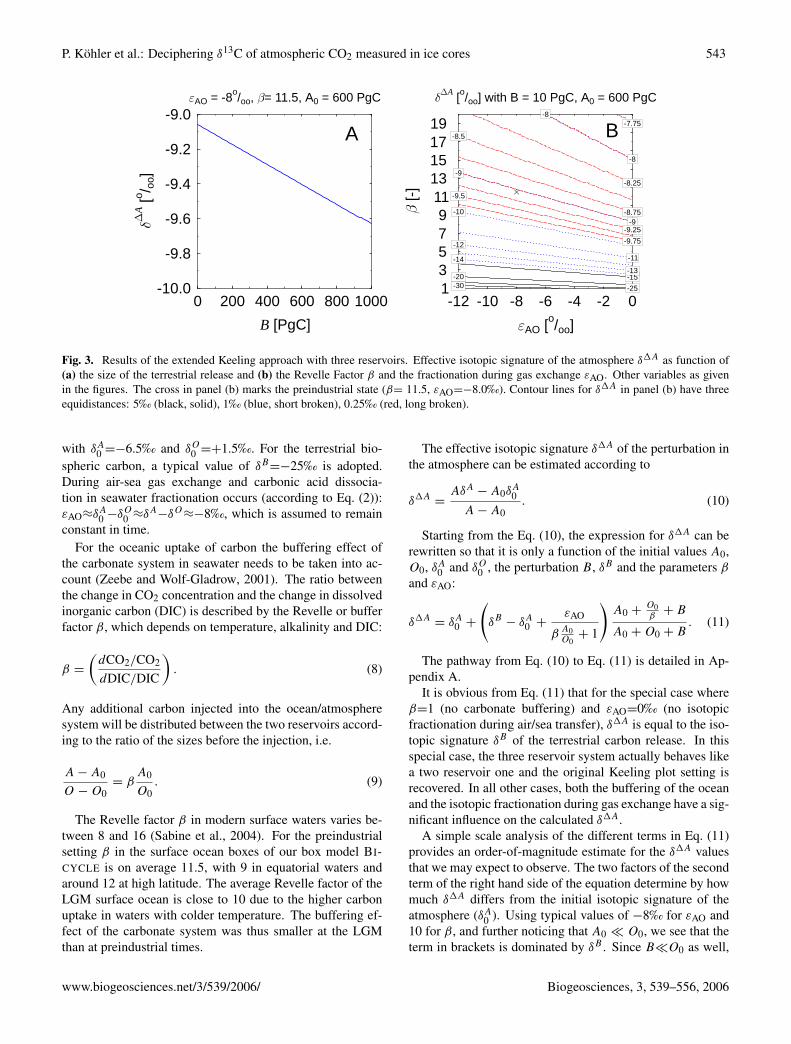
Fig. 3. Results of the extended Keeling approach with three reservoirs. Effective isotopic signature of the atmosphereδ∆A as function of(A) the size of the terrestrial release and(B) the Revelle Factorβ and the fractionation during gas exchangeεAO. Other variable as givenin the figures. The cross in panel (B) marks the preindustrial state (β= 11.5,εAO=−8.0‰). Contour lines forδ∆A in panel (B) have threeequidistances: 5‰ (black, solid), 1‰ (blue, short broken), 0.25‰ (red, long broken).


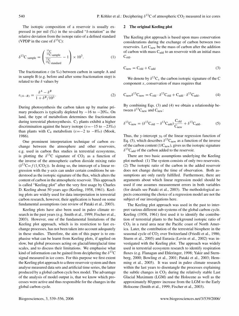
Fig. 3. Results of the extended Keeling approach with three reservoirs. Effective isotopic signature of the atmosphere δ1A as function of(a) the size of the terrestrial release and (b) the Revelle Factor β and the fractionation during gas exchange εAO. Other variables as givenin the figures. The cross in panel (b) marks the preindustrial state (β= 11.5, εAO=−8.0‰). Contour lines for δ1A in panel (b) have threeequidistances: 5‰ (black, solid), 1‰ (blue, short broken), 0.25‰ (red, long broken).

with δA0 =−6.5‰ and δO

0 =+1.5‰. For the terrestrial bio-spheric carbon, a typical value of δB

=−25‰ is adopted.During air-sea gas exchange and carbonic acid dissocia-tion in seawater fractionation occurs (according to Eq. (2)):εAO≈δA

0 −δO0 ≈δA

−δO≈−8‰, which is assumed to remain

constant in time.For the oceanic uptake of carbon the buffering effect of

the carbonate system in seawater needs to be taken into ac-count (Zeebe and Wolf-Gladrow, 2001). The ratio betweenthe change in CO2 concentration and the change in dissolvedinorganic carbon (DIC) is described by the Revelle or bufferfactor β, which depends on temperature, alkalinity and DIC:

β =

(dCO2/CO2

dDIC/DIC

). (8)

Any additional carbon injected into the ocean/atmospheresystem will be distributed between the two reservoirs accord-ing to the ratio of the sizes before the injection, i.e.

A − A0

O − O0= β

A0

O0. (9)

The Revelle factor β in modern surface waters varies be-tween 8 and 16 (Sabine et al., 2004). For the preindustrialsetting β in the surface ocean boxes of our box model BI-CYCLE is on average 11.5, with 9 in equatorial waters andaround 12 at high latitude. The average Revelle factor of theLGM surface ocean is close to 10 due to the higher carbonuptake in waters with colder temperature. The buffering ef-fect of the carbonate system was thus smaller at the LGMthan at preindustrial times.

The effective isotopic signature δ1A of the perturbation inthe atmosphere can be estimated according to

δ1A=

AδA− A0δ

A0

A − A0. (10)

Starting from the Eq. (10), the expression for δ1A can berewritten so that it is only a function of the initial values A0,O0, δA

0 and δO0 , the perturbation B, δB and the parameters β

and εAO:

δ1A= δA

0 +

(δB

− δA0 +

εAO

βA0O0

+ 1

)A0 +

O0β

+ B

A0 + O0 + B. (11)

The pathway from Eq. (10) to Eq. (11) is detailed in Ap-pendix A.

It is obvious from Eq. (11) that for the special case whereβ=1 (no carbonate buffering) and εAO=0‰ (no isotopicfractionation during air/sea transfer), δ1A is equal to the iso-topic signature δB of the terrestrial carbon release. In thisspecial case, the three reservoir system actually behaves likea two reservoir one and the original Keeling plot setting isrecovered. In all other cases, both the buffering of the oceanand the isotopic fractionation during gas exchange have a sig-nificant influence on the calculated δ1A.

A simple scale analysis of the different terms in Eq. (11)provides an order-of-magnitude estimate for the δ1A valuesthat we may expect to observe. The two factors of the secondterm of the right hand side of the equation determine by howmuch δ1A differs from the initial isotopic signature of theatmosphere (δA

0 ). Using typical values of −8‰ for εAO and10 for β, and further noticing that A0 � O0, we see that theterm in brackets is dominated by δB . Since B�O0 as well,



the multiplying factor (A0+O0β

+B)/(A0+O0+B) is of theorder of 1/β. As a consequence δ1A will, in general, deviateby about δB/β or about −2.5‰ from δA

0 .Indeed, when we insert the values for isotopic signatures

and reservoir sizes given above and vary the amount of terres-trial carbon added, the isotopic fractionation during gas ex-change εAO or the Revelle factor β we obtain varying effec-tive isotopic signatures δ1A of the change in the atmosphericcarbon reservoir as shown in Fig. 3. In a typically preindus-trial setting, δ1A varies nearly linearly with B between −9‰and −10‰ (Fig. 3a), reflecting the progressive lightening ofthe overall ocean/atmosphere system when more isotopicallydepleted terrestrial carbon is added. These values are simi-lar to those of Smith et al. (1999) and Fischer et al. (2003)both for the Holocene and the LGM from Taylor Dome icecore data, which have been interpreted as indicative of ter-restrial carbon reservoir changes during these periods. How-ever, from the interpretation of other processes changing theglobal carbon cycle following in Sect. 5.3 it will become ap-parent that there are other processes than the release of ter-restrial carbon that can produce this kind of signal.

There are thus already three preliminary conclusions to bedrawn:

1. The effective isotopic signature δ1A is dependent on theamount of carbon injected and the setting of the systemdescribed by the three reservoirs, their isotopic signa-tures, the fractionation factors, and the Revelle factor.

2. For realistic settings an injection of terrestrial carboninto the atmosphere/ocean produces a δ1A between−8.5 and −10‰. The calculated effective isotopic sig-nature is therefore much more enriched in 13C thanthe carbon released from the terrestrial biosphere withδB

=−25‰. This bias between expectation (δB ) andcalculation (δ1A) is caused by the influence of the oceanand depends only on the system settings described in theprevious conclusion.

3. There exists a limiting value δ1AδB→0 in the effective sig-

nature of the isotopic change in atmospheric δ13C whichis reached if the amount of carbon released to the atmo-sphere converges to zero.

Only for processes that are faster than the equilibration timeof the deep ocean with the atmosphere, substantial amountsof isotopically depleted carbon stay in the atmosphere allow-ing for more negative effective δ1Avalues in the Keeling plot.The latter is seen e.g. for the seasonal variation in CO2 due tothe waxing and waning of the biosphere and, to a smaller ex-tent, also for the input of isotopically depleted anthropogeniccarbon into the atmosphere which operates at typical timescales of decades to centuries.

The effective carbon isotopic signature δ1A based on ourtheoretical consideration as calculated in this section is com-parable with the y0 of a linear regression in a Keeling plot

performed on measured or simulated data sets. This becomesobvious when equation (10) is used to express δA as a func-tion of 1/A:

δA= (δA

0 − δ1A)A0

A+ δ1A, (12)

which is identical to Eq. (5). However, this comparison is,strictly speaking, only valid if the perturbation in the carboncycle is of terrestrial origin. Details in the marine carboncycle, such as spatial variations in the Revelle factor, oceancirculation schemes and the ocean carbon pumps which in-troduce vertical gradients in DIC and 13C in the ocean are notincluded in this analytical approach. This limitation preventsus to apply our theoretical framework directly to discriminatebetween processes of marine origin. Nevertheless, we willuse the linear regression model in the 1/CO2-δ13C-diagramof artificial time series, which were caused by long-term pro-cesses of marine and terrestrial origin to empirically analysehow far these processes can be distinguished by this method.

5 Artificial pCO2 and δ13C times series

Recently, a time-dependent modelling approach gave a quan-titative interpretation of the dynamics of the atmosphericcarbon records over Termination I by forcing the globalocean/atmosphere/biosphere carbon cycle box model BICY-CLE forward in time (Kohler et al., 2005a). The authors iden-tified the impacts of different processes acting on the car-bon cycle on glacial/interglacial time scales and proposed ascenario, which provides an explanation for the evolution ofCO2, δ13C, and 114C over time. The results are in line withvarious other paleo climatic observations.

In the following we will reanalyse the results of Kohleret al. (2005a) by applying the Keeling plot analysis to studywhether this kind of analysis applied on paleo climaticchanges in atmospheric CO2 and δ13C can lead to meaning-ful results. Additional simulations with BICYCLE will beperformed. The advantage of using model-generated artifi-cial time series is, that we know which processes are operat-ing and which process-dependent isotopic fractionations in-fluence the δ13C signals of the results. We highlight how theKeeling plot approach can gain new insights from these datasets and figure out its limitations in paleo climatic research.

Since BICYCLE does not resolve seasonal phenomena weare unable to interpret or, e.g., reconstruct the dynamics ofthe Point Barrow data set of the past few decades. However,we are able to implement the anthropogenic impacts of thelast 250 years as seen in the Law Dome ice core.

5.1 The global carbon cycle box model BICYCLE

The box model of the global carbon cycle BICYCLE consistsof an ocean module with ten homogeneous boxes in threebasins (Atlantic, Southern Ocean, Indo-Pacific) and three dif-ferent vertical layers (surface, intermediate, deep), a glob-




��

��

��

��

��

��

��

��

Box model of the Isotopic Carbon cYCLE BICYCLE

100 m

1000 m

DEEP

SURFACE

MEDIATEINTER−

Rock

carbon

water

C3

FS

SS

NW

W

D

C4

Atmosphere

Atlantic Indo−Pacific

Sediment

40°N50°N 40°S 40°S

SO

Biosphere

16

22

5

10 1

416

96

3 30

9

16

20

1

18

19

15

6

9 9

16 12 5

2

1

3

Fig. 4. A sketch of the BICYCLE model including boundary conditions and preindustrial ocean circulationfluxes (in Sv=106 m2 s−1) in the

ocean module. The globally averaged terrestrial biosphere distinguishes ground vegetation following different photosynthetic pathways (C4,C3), non-woody (NW), and woody (W) parts of trees, and soil compartments (D, FS, SS) with different turnover times.


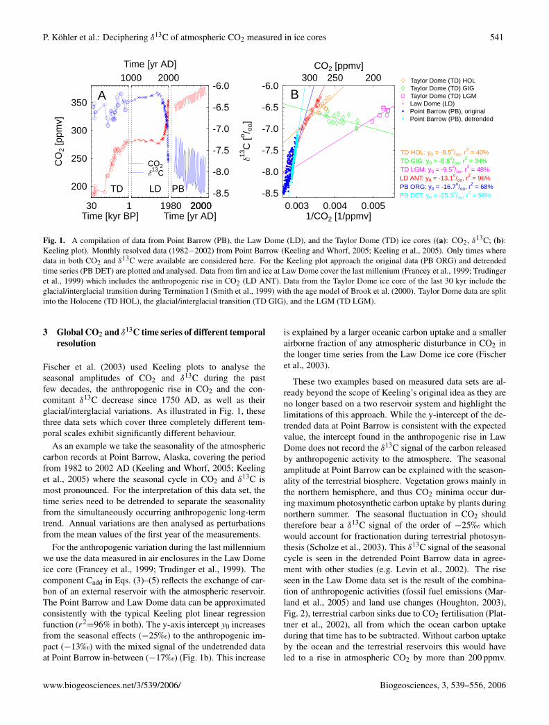
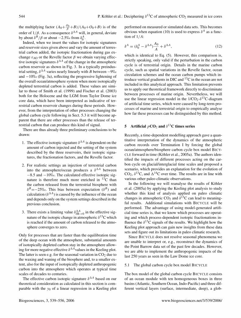
Fig. 4. A sketch of the BICYCLE model including boundary conditions and preindustrial ocean circulation fluxes (in Sv=106 m2 s−1) in theocean module redrawn from Kohler et al. (2006a). The globally averaged terrestrial biosphere distinguishes ground vegetation followingdifferent photosynthetic pathways (C4, C3), non-woody (NW), and woody (W) parts of trees, and soil compartments (D, FS, SS) withdifferent turnover times.

ally averaged atmospheric box and a terrestrial module withseven globally averaged compartments representing groundand tree vegetation and soil carbon with different turnovertimes (Fig. 4). Prognostic variables in the model are DIC,alkalinity, oxygen, phosphate and the carbon isotopes 13Cand 14C in the ocean boxes, and carbon and its carbon iso-topes in the atmosphere and terrestrial reservoirs. The netdifference between sedimentation and dissolution of CaCO3is calculated from variations of the lysocline and determinesthe exchange of DIC and alkalinity between deep ocean andsediment. The model is completely described in Kohler andFischer (2004) and Kohler et al. (2005a). The architectureof BICYCLE is derived from previous box models (Emanuelet al., 1984; Munhoven, 1997). It was adapted to study ques-tions of paleo climate research and uses up-to-date parame-terisations.

We apply disturbances of the climate system throughthe use of forcing functions and paleo climatic records(e.g. changes in temperature, sea level, aeolian dust input inthe Southern Ocean) and prescribe changes in ocean circula-tion over time based on other data- and model-based studies.BICYCLE can then be used to interpret the evolution of at-mospheric CO2, δ13C, and 114C (Kohler et al., 2005a). Itwas further used to simulate variations of atmospheric CO2during the last eight glacial cycles (Wolff et al., 2005; Kohler

and Fischer, 2006), and to analyse the implication of changesin the carbon cycle on atmospheric 114C (Kohler et al.,2006a).

5.2 Anthropogenic emissions – ground truthing of the pa-leo Keeling plot approach

We implement a data-based estimate of the anthropogenicemission since 1750 AD in our model as shown in Fig. 2.BICYCLE calculates pCO2 depending on the dynamics ofthe terrestrial biosphere. In the more realistic case of an ac-tive terrestrial biosphere, which considers an enhanced pho-tosynthesis and thus carbon uptake through CO2 fertilisation,pCO2 in 2000 AD is calculated to 351 µatm (Fig. 5c). A sce-nario with passive terrestrial biosphere, i.e., a constant car-bon storage over time, leads to 388 µatm in the same year(Fig. 5a). In the year 2000 AD the annual mean in the at-mospheric CO2 data at Point Barrow is 371 ppmv, which isapproximately half way between the results of the two dif-ferent simulation scenarios. The scenario with passive ter-restrial biosphere is easier to interpret, since we only haveto consider the anthropogenic carbon flux to the atmosphereand the effect of the oceanic sink. Both scenarios will beanalysed in the following.




260

280

300

320

340

360

380

400pC

O2

[at

m]

13C, -30o/oo

13C, -25o/oo

13C, -20o/oo

pCO2 TB passive

A-10.0

-9.5

-9.0

-8.5

-8.0

-7.5

-7.0

-6.5

13C

[o / oo]

-10.0

-9.5

-9.0

-8.5

-8.0

-7.5

-7.0

-6.5400 350 300

pCO2 [ atm]

13Cant = -20o/ooy0 = -11.8o/oo; r2=99%

13Cant = -25o/ooy0 = -13.7o/oor2=99%

13Cant = -30o/ooy0 = -15.7o/oor2=99%

B

260

280

300

320

340

360

380

400

pCO

2[

atm

]

13C, -30o/oo

13C, -25o/oo

13C, -20o/oo

pCO2 TB active

C1500 1750 2000

Time [yr AD]

-10.0

-9.5

-9.0

-8.5

-8.0

-7.5

-7.0

-6.5

0.0025 0.003 0.00351/pCO2 [1/ atm]

-10.0

-9.5

-9.0

-8.5

-8.0

-7.5

-7.0

-6.5

13C

[o / oo]

13Cant = -20o/ooy0=-9.2o/oo; r2=94%

13Cant = -25o/ooy0=-11.3o/oo; r2=97%

13Cant = -30o/ooy0=-13.5o/oo; r2=98%

D

Fig. 5. Reconstructions of the rise inpCO2 in the atmosphere during the last 500 years with BICYCLE (left: pCO2, δ13C; right: Keelingplot). Anthropogenic fluxes were used as plotted in Fig. 2. Two differentsettings are tested, one with passive terrestrial biosphere TB (top),meaning that carbon storage in the land reservoirs was kept constant, and one with active terrestrial biosphere (bottom), in which a rise inthe internal calculatedpCO2 is enhancing terrestrial carbon uptake via its fertilisation effect. Different simulations with different isotopicsignatures of the anthropogenic emission (−20‰,−25‰,−30‰).


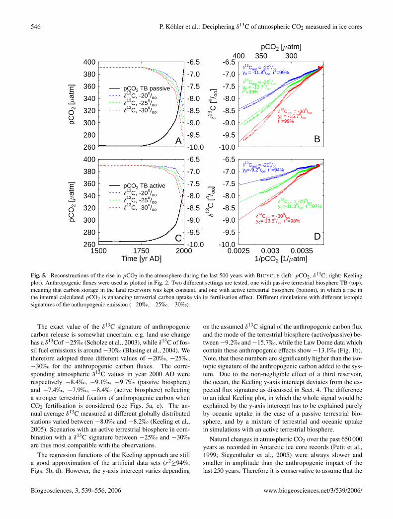
Fig. 5. Reconstructions of the rise in pCO2 in the atmosphere during the last 500 years with BICYCLE (left: pCO2, δ13C; right: Keelingplot). Anthropogenic fluxes were used as plotted in Fig. 2. Two different settings are tested, one with passive terrestrial biosphere TB (top),meaning that carbon storage in the land reservoirs was kept constant, and one with active terrestrial biosphere (bottom), in which a rise inthe internal calculated pCO2 is enhancing terrestrial carbon uptake via its fertilisation effect. Different simulations with different isotopicsignatures of the anthropogenic emission (−20‰, −25‰, −30‰).

The exact value of the δ13C signature of anthropogeniccarbon release is somewhat uncertain, e.g. land use changehas a δ13Cof −25‰ (Scholze et al., 2003), while δ13C of fos-sil fuel emissions is around −30‰ (Blasing et al., 2004). Wetherefore adopted three different values of −20‰, −25‰,−30‰ for the anthropogenic carbon fluxes. The corre-sponding atmospheric δ13C values in year 2000 AD wererespectively −8.4‰, −9.1‰, −9.7‰ (passive biosphere)and −7.4‰, −7.9‰, −8.4‰ (active biosphere) reflectinga stronger terrestrial fixation of anthropogenic carbon whenCO2 fertilisation is considered (see Figs. 5a, c). The an-nual average δ13C measured at different globally distributedstations varied between −8.0‰ and −8.2‰ (Keeling et al.,2005). Scenarios with an active terrestrial biosphere in com-bination with a δ13C signature between −25‰ and −30‰are thus most compatible with the observations.

The regression functions of the Keeling approach are stilla good approximation of the artificial data sets (r2

≥94%,Figs. 5b, d). However, the y-axis intercept varies depending

on the assumed δ13C signal of the anthropogenic carbon fluxand the mode of the terrestrial biosphere (active/passive) be-tween −9.2‰ and −15.7‰, while the Law Dome data whichcontain these anthropogenic effects show −13.1‰ (Fig. 1b).Note, that these numbers are significantly higher than the iso-topic signature of the anthropogenic carbon added to the sys-tem. Due to the non-negligible effect of a third reservoir,the ocean, the Keeling y-axis intercept deviates from the ex-pected flux signature as discussed in Sect. 4. The differenceto an ideal Keeling plot, in which the whole signal would beexplained by the y-axis intercept has to be explained purelyby oceanic uptake in the case of a passive terrestrial bio-sphere, and by a mixture of terrestrial and oceanic uptakein simulations with an active terrestrial biosphere.

Natural changes in atmospheric CO2 over the past 650 000years as recorded in Antarctic ice core records (Petit et al.,1999; Siegenthaler et al., 2005) were always slower andsmaller in amplitude than the anthropogenic impact of thelast 250 years. Therefore it is conservative to assume that the



oceanic uptake of a terrestrial disturbance in the past will al-ways be greater than during the period influenced by humanactivity. We may therefore expect that the y-intercepts of aKeeling plot analysis of these glacial/interglacial processesare closer to the effective isotopic signature calculated fromtheory than the y0 of data for the past few centuries.

5.3 Glacial/interglacial times

There are two factors that make a comparison of artificialtime series with long ice core data sets difficult: First, the airwhich is enclosed in bubbles in the ice can circulate throughthe firn down to the depth where bubble close off occurs(∼ 70−100 m) before it is entrapped in the ice. The bubbleclose off is a slow process with individual bubbles closingat different times and depths. Accordingly the air enclosedin bubbles and in an ice sample is subject to a wide age dis-tribution acting as an efficient low-pass filter on the atmo-spheric record. Therefore, all information from the gaseouscomponents of the ice cores is averaged over a time inter-val of the age of the firn/ice transition zone. This time in-terval is depending on temperature and accumulation rates,but can roughly be estimated by the ratio of the depth ofthe firn/ice transition zone divided by the accumulation rate(Schwander and Stauffer, 1984). At Law Dome, the timeintegral is over a short period only (<20 years) (Etheridgeet al., 1996); at Taylor Dome, it varies between 150 yearsduring the Holocene and 300 years at the LGM (Steig et al.,1998a,b); at EPICA Dome C, where the most recent CO2 andδ13C measurements come from (Monnin et al., 2001; Eyeret al., 2004; Siegenthaler et al., 2005), it ranges between 300and 600 years (Schwander et al., 2001). Second, the CO2and δ13C records retrieved from ice cores are never contin-uous records, but consist of single measurements with large,but irregular gaps in between. In the Taylor Dome ice corethese gaps are on average approximately 1000 years wide. Itwill therefore be of interest to investigate if the temporal res-olution in the data set will be sufficient to resolve informationpotentially retrievable through the Keeling plot approach.

Anthropogenic activities add carbon via land use changeand fossil fuel emissions to the atmosphere. The re-leased carbon is only subsequently absorbed by the ocean.The causes for natural changes in atmospheric CO2 duringglacial/interglacial times were to a large extent located in theocean. Thus, the causes and effects of anthropogenic and nat-ural perturbations of the carbon cycle (including their timing)are in principle different. For the natural glacial/interglacialvariations the carbon content of the atmosphere is determinedby the surface ocean, the atmosphere is also called “slave tothe ocean”, while for the anthropogenic impact the oppositeis the case.

This situation has also consequences for the investigationof different processes causing natural changes in the carboncycle. We concentrate in the following on the individualimpacts of seven important processes. These processes are

changes in terrestrial carbon storage, export production of themarine biota, gas exchange rates and their variation throughvariable sea ice cover, ocean circulation, the physical effectsof variable sea level and ocean temperature, and CaCO3 sedi-mentation and dissolution. Please note, that in these factorialscenarios all processes can be treated un-coupled in our boxmodel, e.g. changes in the circulation scheme will not leadto temperature variations, which might be the case in gen-eral circulation models. A summary of the long-term effectsduring Termination I of all these single process analyses iscompiled in Table 2. Here, however, we discuss only thefirst three processes in greater detail. They are valuable ex-amples of different variability in the carbon cycle: (1) Onlythe changing terrestrial carbon storage strictly resembles theinitial idea of a Keeling plot (addition/subtraction of carbonfrom the atmosphere). (2) Changes in the marine biota illus-trate how variations in the oceanic carbon cycle affects theatmospheric reservoirs. (3) The investigation of the gas ex-change rates, finally, exemplifies a case in which the interfacebetween atmosphere and ocean is perturbed.

5.3.1 Terrestrial biosphere

There are two opposing changes in terrestrial carbon storageto be investigated: carbon uptake and carbon release. Bothmight happen very fast in the course of abrupt climateanomalies, such as so-called Dansgaard/Oeschger events(Dansgaard et al., 1982; Johnsen et al., 1992), duringwhich Greenland temperatures rose and dropped by morethan 15 K in a few decades during the last glacial cycle(Lang et al., 1999; Landais et al., 2004). Terrestrial carbonstorage anomalies during these events were estimated witha dynamic global vegetation model to be of the order of50−100 PgC (Kohler et al., 2005b). The time scales ofthese anomalies are of the order of centuries to millenia.We first analyse a scenario in which 10 PgC are releasedor taken up by the terrestrial pools within one year. Thisshort time frame of one year was chosen to provide baselineexperiments, in which the whole carbon flux is first alteringthe atmospheric reservoir, before oceanic uptake or releaseresponds after year one. The amplitude of the perturbationsis optimised to 10 PgC to guarantee still negligible numericaluncertainties (<0.01‰) in the calculation of the δ13C fluxes.We follow with an experiment of linear carbon release toinvestigate the importance of the time scale for the Keelingplot interpretation. Results of scenarios of carbon uptakeduring Termination I as assumed in Kohler et al. (2005a) arevery similar to the linear experiment and not discussed ingreater detail.

Fast terrestrial carbon release

This is the scenario that comes closest to the originalKeeling plot analysis in terrestrial ecosystem research.There is a source (terrestrial biosphere) which emits CO2



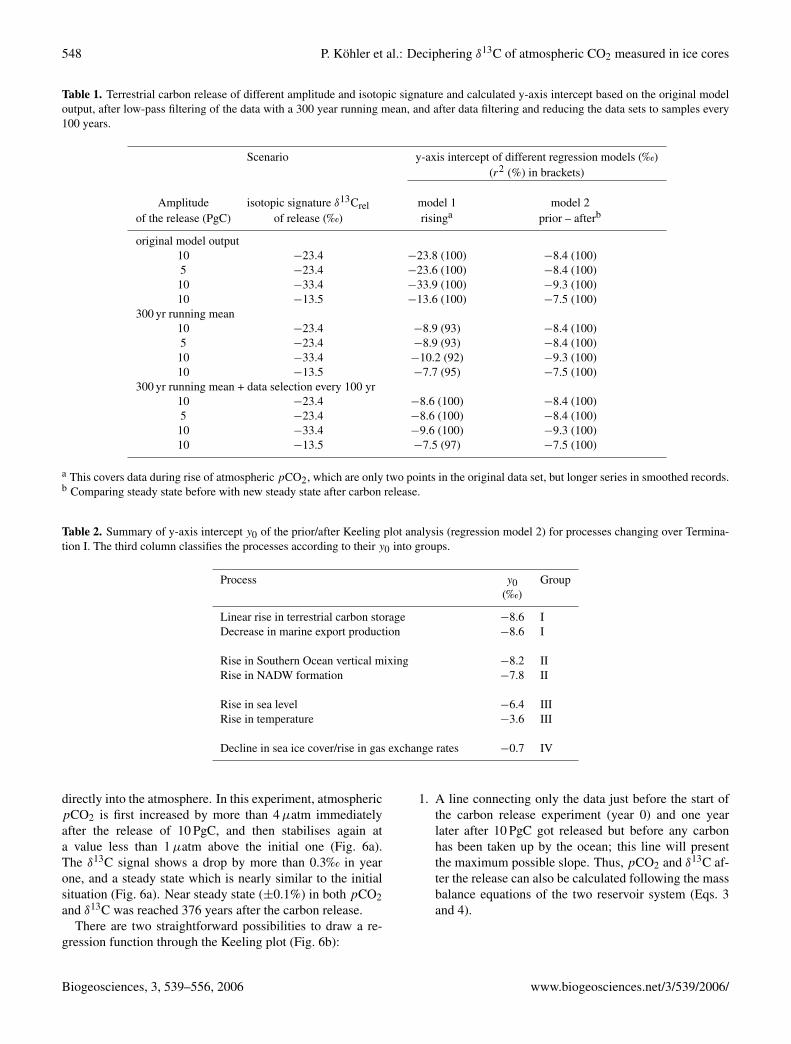
Table 1. Terrestrial carbon release of different amplitude and isotopic signature and calculated y-axis intercept based on the original modeloutput, after low-pass filtering of the data with a 300 year running mean, and after data filtering and reducing the data sets to samples every100 years.

Scenario y-axis intercept of different regression models (‰)(r2 (%) in brackets)

Amplitude isotopic signature δ13Crel model 1 model 2of the release (PgC) of release (‰) risinga prior – afterb

original model output10 −23.4 −23.8 (100) −8.4 (100)5 −23.4 −23.6 (100) −8.4 (100)10 −33.4 −33.9 (100) −9.3 (100)10 −13.5 −13.6 (100) −7.5 (100)

300 yr running mean10 −23.4 −8.9 (93) −8.4 (100)5 −23.4 −8.9 (93) −8.4 (100)10 −33.4 −10.2 (92) −9.3 (100)10 −13.5 −7.7 (95) −7.5 (100)

300 yr running mean + data selection every 100 yr10 −23.4 −8.6 (100) −8.4 (100)5 −23.4 −8.6 (100) −8.4 (100)10 −33.4 −9.6 (100) −9.3 (100)10 −13.5 −7.5 (97) −7.5 (100)

a This covers data during rise of atmospheric pCO2, which are only two points in the original data set, but longer series in smoothed records.b Comparing steady state before with new steady state after carbon release.

Table 2. Summary of y-axis intercept y0 of the prior/after Keeling plot analysis (regression model 2) for processes changing over Termina-tion I. The third column classifies the processes according to their y0 into groups.

Process y0 Group(‰)

Linear rise in terrestrial carbon storage −8.6 IDecrease in marine export production −8.6 I

Rise in Southern Ocean vertical mixing −8.2 IIRise in NADW formation −7.8 II

Rise in sea level −6.4 IIIRise in temperature −3.6 III

Decline in sea ice cover/rise in gas exchange rates −0.7 IV

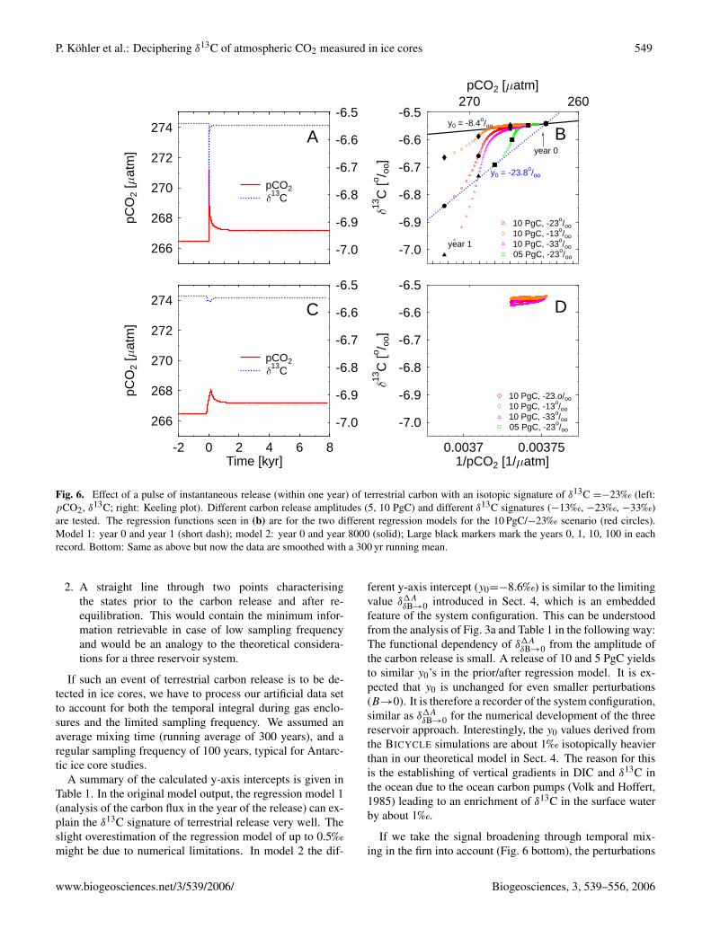
directly into the atmosphere. In this experiment, atmosphericpCO2 is first increased by more than 4 µatm immediatelyafter the release of 10 PgC, and then stabilises again ata value less than 1 µatm above the initial one (Fig. 6a).The δ13C signal shows a drop by more than 0.3‰ in yearone, and a steady state which is nearly similar to the initialsituation (Fig. 6a). Near steady state (±0.1%) in both pCO2and δ13C was reached 376 years after the carbon release.

There are two straightforward possibilities to draw a re-gression function through the Keeling plot (Fig. 6b):

1. A line connecting only the data just before the start ofthe carbon release experiment (year 0) and one yearlater after 10 PgC got released but before any carbonhas been taken up by the ocean; this line will presentthe maximum possible slope. Thus, pCO2 and δ13C af-ter the release can also be calculated following the massbalance equations of the two reservoir system (Eqs. 3and 4).




266

268

270

272

274pC

O2

[at

m]

13CpCO2

A

-7.0

-6.9

-6.8

-6.7

-6.6

-6.5

13C

[o / oo]

-7.0

-6.9

-6.8

-6.7

-6.6

-6.5270 260

pCO2 [ atm]

05 PgC, -23o/oo

10 PgC, -33o/oo

10 PgC, -13o/oo

10 PgC, -23o/oo

y0 = -23.8o/oo

y0 = -8.4o/oo

year 1

year 0

B

266

268

270

272

274

pCO

2[

atm

]

13CpCO2

C

-2 0 2 4 6 8Time [kyr]

-7.0

-6.9

-6.8

-6.7

-6.6

-6.5

13C

[o / oo]

0.0037 0.003751/pCO2 [1/ atm]

-7.0

-6.9

-6.8

-6.7

-6.6

-6.5

05 PgC, -23o/oo

10 PgC, -33o/oo

10 PgC, -13o/oo

10 PgC, -23.o/oo

D

Fig. 6. Effect of a pulse of instantaneous release (within one year) of terrestrial carbon with an isotopic signature ofδ13C =−23‰ (left:pCO2, δ13C; right: Keeling plot). Different carbon release amplitudes (5, 10 PgC)and differentδ13C signatures (−13‰,−23‰,−33‰)are tested. The regression functions seen in(B) are for the two different regression models for the 10 PgC/−23‰ scenario (red circles).Model 1: year 0 and year 1 (short dash); model 2: year 0 and year8000 (solid); Large black markers mark the years 0, 1, 10, 100 in eachrecord. Bottom: Same as above but now the data are smoothed with a 300 yr running mean.


Fig. 6. Effect of a pulse of instantaneous release (within one year) of terrestrial carbon with an isotopic signature of δ13C =−23‰ (left:pCO2, δ13C; right: Keeling plot). Different carbon release amplitudes (5, 10 PgC) and different δ13C signatures (−13‰, −23‰, −33‰)are tested. The regression functions seen in (b) are for the two different regression models for the 10 PgC/−23‰ scenario (red circles).Model 1: year 0 and year 1 (short dash); model 2: year 0 and year 8000 (solid); Large black markers mark the years 0, 1, 10, 100 in eachrecord. Bottom: Same as above but now the data are smoothed with a 300 yr running mean.

2. A straight line through two points characterisingthe states prior to the carbon release and after re-equilibration. This would contain the minimum infor-mation retrievable in case of low sampling frequencyand would be an analogy to the theoretical considera-tions for a three reservoir system.

If such an event of terrestrial carbon release is to be de-tected in ice cores, we have to process our artificial data setto account for both the temporal integral during gas enclo-sures and the limited sampling frequency. We assumed anaverage mixing time (running average of 300 years), and aregular sampling frequency of 100 years, typical for Antarc-tic ice core studies.

A summary of the calculated y-axis intercepts is given inTable 1. In the original model output, the regression model 1(analysis of the carbon flux in the year of the release) can ex-plain the δ13C signature of terrestrial release very well. Theslight overestimation of the regression model of up to 0.5‰might be due to numerical limitations. In model 2 the dif-

ferent y-axis intercept (y0=−8.6‰) is similar to the limitingvalue δ1A

δB→0 introduced in Sect. 4, which is an embeddedfeature of the system configuration. This can be understoodfrom the analysis of Fig. 3a and Table 1 in the following way:The functional dependency of δ1A

δB→0 from the amplitude ofthe carbon release is small. A release of 10 and 5 PgC yieldsto similar y0’s in the prior/after regression model. It is ex-pected that y0 is unchanged for even smaller perturbations(B→0). It is therefore a recorder of the system configuration,similar as δ1A

δB→0 for the numerical development of the threereservoir approach. Interestingly, the y0 values derived fromthe BICYCLE simulations are about 1‰ isotopically heavierthan in our theoretical model in Sect. 4. The reason for thisis the establishing of vertical gradients in DIC and δ13C inthe ocean due to the ocean carbon pumps (Volk and Hoffert,1985) leading to an enrichment of δ13C in the surface waterby about 1‰.

If we take the signal broadening through temporal mix-ing in the firn into account (Fig. 6 bottom), the perturbations




260

280

300

320

340pC

O2

[at

m]

13CpCO2

A

-2 0 2 4 6 8Time [kyr]

-7.0

-6.9

-6.8

-6.7

-6.6

-6.5

13C

[o / oo]

0.003 0.0035 0.0041/pCO2 [1/ atm]

-7.0

-6.9

-6.8

-6.7

-6.6

-6.5350 300 250

pCO2 [ atm]

y0 = -8.6o/oo, r2 = 99%

year 0

year 8000

B

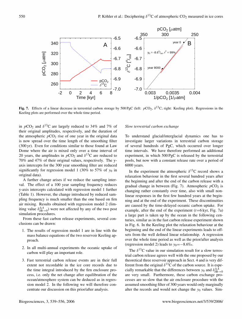
Fig. 7. Effects of a linear decrease in terrestrial carbon storage by 500 PgC (left: pCO2, δ13C; right: Keeling plot). Regressions in theKeeling plots are performed over the whole time period.


Fig. 7. Effects of a linear decrease in terrestrial carbon storage by 500 PgC (left: pCO2, δ13C; right: Keeling plot). Regressions in theKeeling plots are performed over the whole time period.

in pCO2 and δ13C are largely reduced to 34% and 7% oftheir original amplitudes, respectively, and the duration ofthe atmospheric pCO2 rise of one year in the original datais now spread over the time length of the smoothing filter(300 yr). Even for conditions similar to those found at LawDome where the air is mixed only over a time interval of20 years, the amplitudes in pCO2 and δ13C are reduced to70% and 47% of their original values, respectively. The y-axis intercepts for the 300 year smoothing filter are reducedsignificantly for regression model 1 (30% to 57% of y0 inoriginal data).

A further change arises if we reduce the sampling inter-val. The effect of a 100 year sampling frequency reducesy-axis intercepts calculated with regression model 1 further(Table 1). However, the change introduced by reduced sam-pling frequency is much smaller than the one based on firnair mixing. Results obtained with regression model 2 (lim-iting value δ1A

δB→0) were not affected by any of the two postsimulation procedures.

From these fast carbon release experiments, several con-clusions can be drawn:

1. The results of regression model 1 are in line with themass balance equations of the two reservoir Keeling ap-proach.

2. In all multi-annual experiments the oceanic uptake ofcarbon will play an important role.

3. Fast terrestrial carbon release events are in their fullextent not recordable in the ice core records due tothe time integral introduced by the firn enclosure pro-cess, i.e. only the net change after equilibration of theocean/atmosphere system can be deduced as in regres-sion model 2. In the following we will therefore con-centrate our discussion on this prior/after analysis.

Slow terrestrial carbon exchange

To understand glacial/interglacial dynamics one has toinvestigate larger variations in terrestrial carbon storageof several hundreds of PgC, which occurred over longertime intervals. We have therefore performed an additionalexperiment, in which 500 PgC is released by the terrestrialpools, but now with a constant release rate over a period of6000 years.

In the experiment the atmospheric δ13C record shows arelaxation behaviour in the first several hundred years afterthe beginning and after the end of the carbon release with agradual change in between (Fig. 7). Atmospheric pCO2 ischanging rather constantly over time, also with small non-linear responses in the first few hundred years at the begin-ning and at the end of the experiment. These discontinuitiesare caused by the time-delayed oceanic carbon uptake. Forexample, after the end of the experiment (t=6 kyr, Fig. 7a)a large part is taken up by the ocean in the following cen-turies, similar as in the fast carbon release experiment shownin Fig. 6. In the Keeling plot the relaxation behaviour at thebeginning and the end of the linear experiments leads to off-sets from the well defined linear relationship. A regressionover the whole time period as well as the prior/after analysis(regression model 2) leads to y0=−8.6‰.

The δ13C value in our simulation result for a slow terres-trial carbon release agrees well with the one proposed by ourtheoretical three reservoir approach in Sect. 4 and is very dif-ferent from the original δ13C of the carbon source. It is espe-cially remarkable that the differences between y0 and δ1A

δB→0are very small. Furthermore, these carbon exchange pro-cesses are so slow that the air enclosure procedure with theassumed smoothing filter of 300 years would only marginallyalter the records and would not change the y0 values. Sim-




240

250

260

270pC

O2

[at

m]

13CpCO2

A20 18 16 14 12 10

Time [kyr BP]

-6.6

-6.5

-6.4

-6.3

13C

[o / oo]

0.00375 0.0041/pCO2 [1/ atm]

-6.6

-6.5

-6.4

-6.3270 250

pCO2 [ atm]

y0 = -8.6o/oo

20 kyr BP

10 kyr BPB

Fig. 8. Effects of iron fertilisation in the Southern Ocean on atmospheric carbon records with scenario taken from Kohler et al. (2005a) (A:pCO2, δ13C; B: Keeling plot). Blue dots and regression in (B) over the first 50 years during pCO2 rise only.


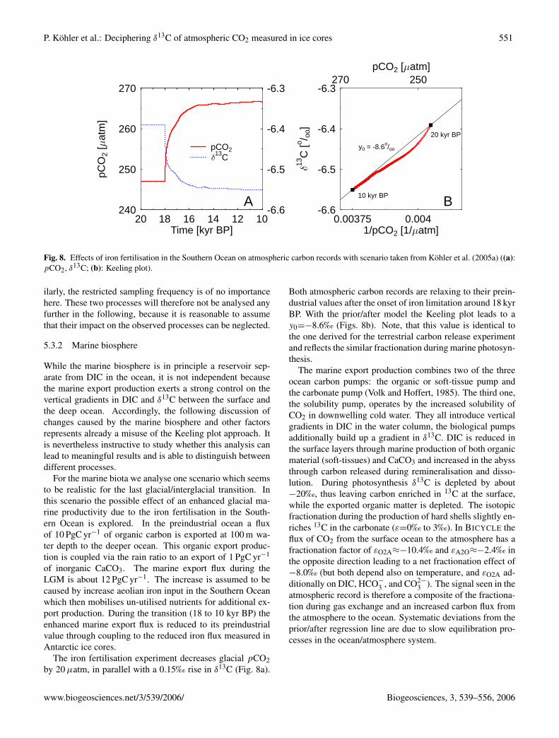
Fig. 8. Effects of iron fertilisation in the Southern Ocean on atmospheric carbon records with scenario taken from Kohler et al. (2005a) ((a):pCO2, δ13C; (b): Keeling plot).

ilarly, the restricted sampling frequency is of no importancehere. These two processes will therefore not be analysed anyfurther in the following, because it is reasonable to assumethat their impact on the observed processes can be neglected.

5.3.2 Marine biosphere

While the marine biosphere is in principle a reservoir sep-arate from DIC in the ocean, it is not independent becausethe marine export production exerts a strong control on thevertical gradients in DIC and δ13C between the surface andthe deep ocean. Accordingly, the following discussion ofchanges caused by the marine biosphere and other factorsrepresents already a misuse of the Keeling plot approach. Itis nevertheless instructive to study whether this analysis canlead to meaningful results and is able to distinguish betweendifferent processes.

For the marine biota we analyse one scenario which seemsto be realistic for the last glacial/interglacial transition. Inthis scenario the possible effect of an enhanced glacial ma-rine productivity due to the iron fertilisation in the South-ern Ocean is explored. In the preindustrial ocean a fluxof 10 PgC yr−1 of organic carbon is exported at 100 m wa-ter depth to the deeper ocean. This organic export produc-tion is coupled via the rain ratio to an export of 1 PgC yr−1

of inorganic CaCO3. The marine export flux during theLGM is about 12 PgC yr−1. The increase is assumed to becaused by increase aeolian iron input in the Southern Oceanwhich then mobilises un-utilised nutrients for additional ex-port production. During the transition (18 to 10 kyr BP) theenhanced marine export flux is reduced to its preindustrialvalue through coupling to the reduced iron flux measured inAntarctic ice cores.

The iron fertilisation experiment decreases glacial pCO2by 20 µatm, in parallel with a 0.15‰ rise in δ13C (Fig. 8a).

Both atmospheric carbon records are relaxing to their prein-dustrial values after the onset of iron limitation around 18 kyrBP. With the prior/after model the Keeling plot leads to ay0=−8.6‰ (Figs. 8b). Note, that this value is identical tothe one derived for the terrestrial carbon release experimentand reflects the similar fractionation during marine photosyn-thesis.

The marine export production combines two of the threeocean carbon pumps: the organic or soft-tissue pump andthe carbonate pump (Volk and Hoffert, 1985). The third one,the solubility pump, operates by the increased solubility ofCO2 in downwelling cold water. They all introduce verticalgradients in DIC in the water column, the biological pumpsadditionally build up a gradient in δ13C. DIC is reduced inthe surface layers through marine production of both organicmaterial (soft-tissues) and CaCO3 and increased in the abyssthrough carbon released during remineralisation and disso-lution. During photosynthesis δ13C is depleted by about−20‰, thus leaving carbon enriched in 13C at the surface,while the exported organic matter is depleted. The isotopicfractionation during the production of hard shells slightly en-riches 13C in the carbonate (ε=0‰ to 3‰). In BICYCLE theflux of CO2 from the surface ocean to the atmosphere has afractionation factor of εO2A≈−10.4‰ and εA2O≈−2.4‰ inthe opposite direction leading to a net fractionation effect of−8.0‰ (but both depend also on temperature, and εO2A ad-ditionally on DIC, HCO−

3 , and CO2−

3 ). The signal seen in theatmospheric record is therefore a composite of the fractiona-tion during gas exchange and an increased carbon flux fromthe atmosphere to the ocean. Systematic deviations from theprior/after regression line are due to slow equilibration pro-cesses in the ocean/atmosphere system.




250

260

270

280

290

300

310pC

O2

[at

m] 13C S only

13C N onlypCO2 S onlypCO2 N only A

-2 0 2 4 6 8Time [kyr]

-6.6

-6.4

-6.2

-6.0

-5.8

-5.6

13C

[o / oo]

0.0033 0.0036 0.00391/pCO2 [1/ atm]

-6.6

-6.4

-6.2

-6.0

-5.8

-5.6

300 280 260pCO2 [ atm]

S onlyN only

y0 = -6.1o/oo

y0 = -23.8o/oo

B

year 0

year 0

year 8000

Fig. 9. Simulated effects of an instantaneous change in sea ice cover from total coverage to preindustrial values in the North Atlantic (Nonly), or the Southern Ocean (S only) (left:pCO2, δ13C; right: Keeling plot).


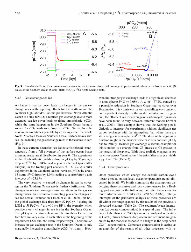
Fig. 9. Simulated effects of an instantaneous change in sea ice cover from total coverage to preindustrial values in the North Atlantic (Nonly), or the Southern Ocean (S only) (left: pCO2, δ13C; right: Keeling plot).

5.3.3 Gas exchange/sea ice

A change in sea ice cover leads to changes in the gas ex-change rates with opposing effects for the northern and thesouthern high latitudes. As the preindustrial North AtlanticOcean is a sink for CO2 a reduced gas-exchange due to moreextended sea ice cover leads to rising atmospheric pCO2,while the same happening in the Southern Ocean being asource for CO2 leads to a drop in pCO2. We explore themaximum amplitudes possible by covering either the wholeNorth Atlantic Ocean or Southern Ocean surface boxes withsea ice, reducing the gas exchange rates in these areas to zero(Fig. 9).

In these extreme scenarios sea ice cover is relaxed instan-taneously from a full coverage of the surface ocean boxesto preindustrial areal distribution in year 0. The experimentin the North Atlantic yields a drop in pCO2 by 35 µatm, adrop in δ13C by 0.04‰, and a y-axis intercept (prior/afteranalysis) in the Keeling plot analysis of −6.1‰. A similarexperiment in the Southern Ocean increases pCO2 by about15 µatm, δ13C drops by 1.0‰ leading to a prior/after y-axisintercept of −23.8‰.

The very negative y0 caused by changes in sea ice cover-age in the Southern Ocean needs further clarification. Thechanges in sea ice coverage cause variations in the gas ex-change rates. In a scenario resampling plausible changes insea ice across Termination I (Kohler et al., 2005a, 2006b),the global exchange flux rises from 52 PgC yr−1 during theLGM to 58 PgC yr−1 at t=10 kyr BP in the scenario, whichconsiders only changes in sea ice in the Southern Ocean.The pCO2 of the atmosphere and the Southern Ocean sur-face box are very close to each other at the beginning of theexperiment (270 and 266 µatm, respectively). Therefore, anincrease in gas exchange rate in the Southern Ocean is onlymarginally increasing atmospheric pCO2(<1 µatm). How-

ever, the stronger gas exchange leads to a significant decreasein atmospheric δ13C by 0.08‰. A y0 of −77.2‰ caused bya plausible reduction in Southern Ocean sea ice cover overTermination I is consistent in our modelling environment,but dependent strongly on the model architecture. In gen-eral, the effects of sea ice coverage on carbon cycle dynamicshave been found to vary between different models (Archeret al., 2003). This example shows, that the Keeling plot isdifficult to interpret for experiments without significant netcarbon exchange with the atmosphere, but where there arestill changes in atmospheric δ13C. The slope of the regressionfunction might in the most extreme case of a constant pCO2rise to infinity. Besides gas exchange a second example forthis situation is a change from C3 grasses to C4 grasses inthe terrestrial biosphere. With these realistic changes in seaice cover across Termination I the prior/after analysis yieldsa y0 of −0.7‰ (Table 2).

5.3.4 Other processes

Other processes which change the oceanic carbon cycle(ocean circulation, sea level, ocean temperature) are not dis-cussed in detail. We briefly summarise the assumptions un-derlying these processes and their consequences for a Keel-ing plot analysis in the following, but refer the readers formore information to Kohler et al. (2005a, 2006b). The y-intercepts of the prior/after analysis of these processes areall within the range spanned by the results of the previouslydiscussed changes (Table 2). The sediment/ocean interac-tion (carbonate compensation) is a special case. The influ-ence of the fluxes of CaCO3 cannot be analysed separatelyas CaCO3 fluxes between deep ocean and sediment are gen-erated by the model as response to changes in the deep oceanCO2−

3 concentration. Carbonate compensation is acting asan amplifier of the results of all other processes with re-



spect to the changes in pCO2. It is therefore not possible tofind a pure signal of carbonate compensation in atmosphericrecords. The impact of this process could in principle be esti-mated by subtracting results of simulations, in which carbon-ate compensation is either on or off from each other, but werefrain from this. All other process analyses (including ter-restrial and marine biota and sea ice) were performed withoutcarbonate compensation.

In general, it has to be said that especially abruptchanges in ocean circulation lead to fast fluctuations inboth atmospheric carbon records and thus also to Keelingplots, which are not easily represented by linear regressionmodels. However, our comparison here is restricted tothe long-term effects, in which atmosphere and ocean arealready equilibrated.

Ocean circulation:Based on evidences from various sediment records andocean general circulation models we assume changes (1)in the strength of the North Atlantic Deep Water (NADW)formation and (2) in the Southern Ocean vertical mixing.(1): NADW formation is increased from its glacial strength(10 Sv) during the LGM to intermediate levels of 16 Sv atthe beginning of the Holocene neglecting potential millennialscale fluctuations during the Bølling/Allerød and YoungerDryas climate anomalies. This leads to a rise in atmosphericpCO2 by 12 µatm and a small drop in δ13C (−0.06‰). Theprior/after analysis in the Keeling plot leads to a y-axis in-tercept of −7.8‰. (2): Southern Ocean vertical mixing raterises from 9 Sv (LGM) to 29 Sv (Holocene) and leads to arise in pCO2 by about 30 µatm and a drop in δ13C by morethan 0.2‰. Here, the Keeling plot interpretation gives us ay-axis intercept of −8.2‰ for the prior/after analysis.

The overturning circulation distributes carbon in theocean. Its effect on the atmospheric carbon reservoirs,however, is opposite to that of the three ocean carbon pumps.While the pumps introduce vertical gradients in DIC andδ13C, the overturning circulation is reducing these verticalgradients again through the ventilation of the deep oceanwhich brings water rich in DIC and depleted in 13C back tothe surface. A weakening of the ventilation reduces theseupwelling processes and leads to lower pCO2 and higherδ13C values as seen in the experiments.

Sea level:Sea level rose from 20 kyr BP to 10 kyr BP by about 85 m.This leads in our model to a drop in pCO2 by about 13 µatmand nearly no change in the δ13C. The y-axis intercept ina Keeling plot with prior/after analysis or regression overwhole time period is −6.4‰.

The rising sea level leads to a dilution of the concentrationof all species in the ocean and a decrease in salinity by about2.3%. The ocean can then store more carbon.

Ocean temperature:The rise of the ocean temperature by 3 to 5 K during the sim-ulated 20 to 10 kyr BP leads to a rise in pCO2 of 32 µatm,and a rise in δ13C of 0.4‰, the latter leading the first byabout 1000 years. The Keeling plot analysis gives us a y0 of−3.6‰ for the regression in the prior/after analysis.

Due to the temperature dependent solubility of CO2 warmwater stores less carbon than cold water. A rise in oceantemperature therefore weakens the solubility pump and leadsto an out-gassing of CO2. The rise in δ13C is mainly causedby the temperature-dependent isotopic fractionation duringgas exchange between the surface ocean and the atmosphere.

6 Conclusions

In this study we analysed processes which alter the atmo-spheric content of carbon dioxide and δ13C of CO2 usingartificial time series produced with a global carbon cycle boxmodel. For the investigation of these artificial time seriesand their potential to be interpreted using the Keeling plotapproach, the absolute validity of our simulation scenariosis not important. By using a simple carbon cycle model webenefit from the fact that individual processes acting on thecarbon cycle can be switched on and off and their hypothet-ical impacts can be analysed individually. We furthermoredeveloped a theoretical framework to extend the applicationof the Keeling plot approach to long-term effects of terres-trial carbon release.

All processes have been analysed with respect to their im-pact to the Keeling plot analysis. A summary is found inTable 2. The y-intercepts of this analysis in the case of ter-restrial carbon release is fundamentally different from the ex-pected value, which should contain the δ13C of the terrestrialsource. The bias can be understood based on theoretical con-siderations of a three reservoir system which also includesoceanic carbon uptake. These considerations are the paleoextension of the Keeling plot approach to envisage long-termeffects of terrestrial processes. From them δ1A is calculated,the long-term change in the isotopic signature of atmosphericCO2 caused by the underlying process, called effective iso-topic signature. δ1A

δB→0 obtained from theory is comparableto the y-axis intercept y0 in a classical Keeling plot. So far,changes in the marine carbon cycle can not be understoodwith our simple three reservoir approach.

However, the comparison of y-intercepts derived from dif-ferent processes is used to investigate if this method can beused to distinguish between different processes operation onlong time scales on the global carbon cycle. The y0’s of theprior/after analysis of our single process analysis vary be-tween −0.7 and −8.6‰. Based on the calculated y0 valuesthe processes can be subdivided into four groups (Table 2):(I) Processes in which the biology is involved (marine andterrestrial) have identical y0’s (−8.6‰) and are therefore in-



distinguishable. (II) Changes in the ocean circulation lead toy0’s which are slightly more positive (−7.8 to −8.2‰). Pro-cesses belonging to the groups I and II might in real data setsalso be indistinguishable due to measuremental uncertainties.(III) Sea level (−6.4‰) and ocean temperature (−3.6‰)have in their long-term behaviour intermediate y0’s, clearlyhigher than those of the first two groups. (IV) Gas ex-change/sea ice cover yields to the highest y0, but it shouldbe kept in mind that this process is a compound of sub-processes which have distinctively different y0 values (seaice cover in different hemispheres, y0 (north)=−4.8‰; y0(south)=−77.2‰). Furthermore, the terrestrial carbon stor-age very likely changed in a non-linear way during the lastglacial/interglacial transition and not in a linear way as as-sumed here. This is also supported by a simulation studiesusing a dynamical global vegetation model (Kohler et al.,2005b). High frequency changes on a centennial to millen-nial time scale are very likely smoothed out in the ice corerecords due to the average mixing time of the air of severalcenturies and the limited sampling frequency.

From the understanding which emerges here, it seemsunlikely, that the interpretation of δ13C measured duringglacial/interglacial transitions can be enhanced very muchwith the Keeling plot approach. The identification of a singleprocess which might be responsible for the observed fluctu-ations in atmospheric CO2 and δ13C can not be based on aKeeling plot analysis. Most processes acted simultaneouslyon the global carbon cycle during the transition and the un-certainties in data retrieval, y-axis intercept, and δ13C are toolarge to come to a sound and unequivocal process identifica-tion.

Appendix A Calculating the effective isotopic signatureof the three reservoir system

The effective isotopic signature δ1A of the perturbation B,defined by Eq. (10) from Sect. 4

δ1A=

AδA− A0δ

A0

A − A0

can be rewritten such that it is only a function of the initialvalues (A0, O0, δA

0 , δO0 ), the forcing (B, δB ) and parameters

(β, εAO). To start, Eq. (10) is rewritten under the equivalentexpression

δ1A= δA

0 +A

A − A0(δA

− δA0 ) (A1)

The reformulation then proceeds in two stages, the first onedealing with A/(A − A0), the second one with (δA

− δA0 ).

For the first stage, we start by rewriting and combiningEqs. (6) and (9) into a linear system of equations in theanomalies (A − A0) and (O − O0)

(O − O0) + (A − A0) = B

βA0

O0(O − O0) − (A − A0) = 0

The solutions of this system are

O − O0 = B1

βA0O0

+ 1(A2)

and

A − A0 = Bβ

A0O0

βA0O0

+ 1. (A3)

To conclude the first stage, it is sufficient to rewrite A/(A −

A0) as

A

A − A0=

A0A − A0

+ 1, (A4)

and use (A3) to replace (A − A0). After reduction and sim-plification, we find that

A

A − A0=

A0 +O0β

+ B

B. (A5)

The second stage proceeds from Eq. (7)

AδA+ OδO

= A0δA0 + O0δ

O0 + BδB ,

where we first substitute δO= δA

−εAO and δO0 = δA

0 −εAO .After collecting the terms in δA, δA

0 and εAO we then get

(A + O)δA− (A0 + O0)δ

A0 − (O − O0)εAO = BδB .

To continue, we substitute δA= (δA

−δA0 )+δA

0 and rearrangeto get

(A + O)(δA− δA

0 ) − (O − O0)εAO

+ ((A + O) − (A0 + O0))δA0 = BδB .

We then use Eqs. (6)

A + O = A0 + O0 + B

and (A2) to substitute (A + O) and (O − O0) respectively.After simplification, we get

(A0 + O0 + B)(δA− δA

0 ) = B(δB− δA

0 +εAO

βA0O0

+ 1),

from which we may immediately deduce that

δA− δA

0 =B

A0 + O0 + B

(δB

− δA0 +

εAO

βA0O0

+ 1

). (A6)

Finally, by insertion of Eqs. (A5) and (A6) into (A1) we ob-tain the desired expression

δ1A= δA

0 +

(δB

− δA0 +

εAO

βA0O0

+ 1

)A0 +

O0β

+ B

A0 + O0 + B. (A7)



Acknowledgements. We thank J. Severinghaus for ideas on thethree box model calculations, J. Freitag for discussions on firnifica-tion and bubble close off, J. Bijma for his editorial effort and twoanonymous referees for their clarifying comments. This study isfunded by the German Ministry of Education and Research throughthe German Climate Research Programme DEKLIM (projectRESPIC). G. Munhoven is a Research Associate with the BelgianNational Fund for Scientific Research (FNRS).

Edited by: J. Bijma

References

Archer, D. E., Martin, P. A., Milovich, J., Brovkin, V., Plattner, G.-K., and Ashendel, C.: Model sensitivity in the effect of Antarcticsea ice and stratification on atmospheric pCO2, Paleoceanogra-phy, 18, 1012, doi:10.1029/2002PA000760, 2003.

Blasing, T. J., Broniak, C., and Marland, G.: Estimates of monthlycarbon dioxide emissions and associated δ13C values from fossil-fuel consumption in the U.S.A, in: Trends: A Compendium ofData on Global Change, Carbon Dioxide Information AnalysisCenter, Oak Ridge National Laboratory, U.S. Department of En-ergy, Oak Ridge, Tenn., USA, 2004.

Bowling, D. R., Tans, P. P., and Monson, R. K.: Partitioning netecosystem carbon exchange with isotopic fluxes of CO2, GlobalChange Biol., 7, 127–145, 2001.

Brook, E. J., Harder, S., Serveringhaus, J., Steig, E. J., and Sucher,C. M.: On the origin and timing of rapid changes in atmosphericmethane during the last glacial period, Global Biogeochem. Cy-cles, 14, 559–572, 2000.

Dansgaard, W., Clausen, H. B., Gundestrup, N., Hammer, C. U.,Johnsen, S. F., Kristinsdottir, P. M., and Reeh, N.: A new Green-land deep ice core, Science, 218, 1273–1277, 1982.

Emanuel, W. R., Killough, G. G., Post, W. M., and Shugart, H. H.:Modeling terrestrial ecosystems in the global carbon cycle withshifts in carbon storage capacity by land-use change, Ecology,65, 970–983, 1984.

Etheridge, D. M., Steele, L. P., Langenfelds, R. L., Francey, R. J.,Barnola, J.-M., and Morgan, V. I.: Natural and anthropogenicchanges in atmospheric CO2 over the last 1000 years from air inAntarctic ice and firn, J. Geophys. Res., D101, 4115–4128, 1996.

Eyer, M., Leuenberger, M., Nyfeler, P., and Stocker, T.: Comparisonof two δ13CO2 records measured on air from the EPICA DomeC and Kohnen Station ice cores, Geophys. Res. Abstr., 6, 01 990,2004.

Fischer, H., Wahlen, M., and Smith, J.: Reconstruction ofglacial/interglacial changes in the global carbon cycle from CO2and δ13CO2 in Antarctic ice cores, Memoirs of the National In-stitute for Polar Research, Special Issue, 57, 121–138, 2003.

Flanagan, L. B. and Ehleringer, J. R.: Ecosystem-atmosphere CO2exchange: interpretating signals of change using stable isotoperatios, Trends in Ecology and Evolution, 13, 10–14, 1998.

Francey, R. J., Allison, C. E., Etheridge, D. M., Trudinger, C. M.,Enting, I. G., Leuenberger, M., Langenfelds, R. L., Michel, E.,and Steele, L. P.: A 1000-year high precision record of δ13C inatmospheric CO2, Tellus, 51B, 170–193, 1999.

Friedli, H., Lotscher, H., Oeschger, H., Siegenthaler, U., and Stauf-fer, B.: Ice core record of the 13C/12C ratio of atmospheric CO2in the past two centuries, Nature, 324, 237–238, 1986.

Hemming, D., Yakir, D., Ambus, P., Aurela, M., Besson, C.,Black, K., Buchmann, N., Burlett, R., Cescatti, A., Clement, R.,Gross, P., Granier, A., Grunwald, T., Havrankova, K., Janous,D., Janssens, I. A., Knohl, A., Kostner, B., Kowalski, A., Lau-rila, T., Mata, C., Marcolla, B., Matteucci, G., Moncrieff, J.,Moors, E. J., Osborne, B., Pereira, J. S., Pihlatie, M., Pile-gaard, K., Ponti, F., Rosova, U., Rossi, F., Scartazza, A., andVesala, T.: Pan-European δ13C values of air and organic matterfrom forest ecosystems, Global Change Biol., 11, 1065–1093,doi:10.1111/j.1365–2486.2005.00 971.x, 2005.

Houghton, R. A.: Revised estimates of the annual net flux of carbonto the atmosphere from changes in land use and land manage-ment 1850–2000, Tellus, 55B, 378–390, 2003.

Johnsen, S. J., Clausen, H. B., Dansgaard, W., Fuhrer, K., Gunde-strup, N., Hammer, C. U., Iversen, P., Jouzel, J., Stauffer, B., andSteffensen, J. P.: Irregular glacial interstadials recorded in a newGreenland ice core, Nature, 359, 311–313, 1992.

Keeling, C. D.: The concentration and isotopic abundance of carbondioxide in rural areas, Geochim. Cosmochim. Acta, 13, 322–334,1958.

Keeling, C. D.: The concentration and isotopic abundance of carbondioxide in rural and marine air, Geochim. Cosmochim. Acta, 24,277–298, 1961.

Keeling, C. D. and Whorf, T. P.: Atmospheric CO2 records fromsites in the SIO air sampling network, in Trends: A Compendiumof Data on Global Change, Carbon Dioxide Information Analy-sis Center, Oak Ridge National Laboratory, U.S. Department ofEnergy, Oak Ridge, Tenn., USA, 2005.

Keeling, C. D., Bollenbacher, A. F., and Whorf, T. P.: Monthlyatmospheric 13C/12C isotopic ratios for 10 SIO stations, in:Trends: A Compendium of Data on Global Change, CarbonDioxide Information Analysis Center, Oak Ridge National Lab-oratory, U.S. Department of Energy, Oak Ridge, Tenn., USA,2005.

Kohler, P. and Fischer, H.: Simulating changes in theterrestrial biosphere during the last glacial/interglacialtransition, Global and Planetary Change, 43, 33–55,doi:10.1016/j.gloplacha.2004.02.005, 2004.

Kohler, P. and Fischer, H.: Simulating low frequency changes inatmospheric CO2 during the last 740 000 years, Clim. Past, 2,57–78, 2006,http://www.clim-past.net/2/57/2006/.

Kohler, P., Fischer, H., Munhoven, G., and Zeebe, R. E.: Quanti-tative interpretation of atmospheric carbon records over the lastglacial termination, Global Biogeochem. Cycles, 19, GB4020,doi:10.1029/2004GB002345, 2005a.

Kohler, P., Joos, F., Gerber, S., and Knutti, R.: Simulated changesin vegetation distribution, land carbon storage, and atmosphericCO2 in response to a collapse of the North Atlantic thermohalinecirculation, Clim. Dyn., 25, 689–708, doi:10.1007/s00 382–005–0058–8, 2005b.

Kohler, P., Muscheler, R., and Fischer, H.: A model-based interpre-tation of low frequency changes in the carbon cycle during thelast 120 000 years and its implications for the reconstruction ofatmospheric 114C, Geochem., Geophys., Geosyst., 7, Q11N06,doi:10.1029/2005GC001228, 2006a.

Kohler, P., Schmitt, J., and Fischer, H.: On the application and in-terpretation of Keeling plots in paleo climatic research — Deci-phering δ13C of atmospheric CO2 measured in ice cores, Bio-


http://www.clim-past.net/2/57/2006/


geosciences Discuss., 3, 513–573, 2006b.Landais, A., Barnola, J. M., Masson-Delmotte, V., Jouzel, J., Chap-

pellaz, J., Caillon, N., Huber, C., Leuenberger, M., and Johnsen,S. J.: A continuous record of temperature evolution over a se-quence of Dansgaard-Oeschger events during Marine IsotopeStage 4 (76 to 62 kyr BP), Geophys. Res. Lett., 31, L22 211,doi:10.1029/2004GL021193, 2004.

Lang, C., Leuenberger, M., Schwander, J., and Johnsen, S.: 16◦Crapid temperature variation in central Greenland 70,000 yearsago, Science, 286, 934–937, 1999.

Levin, I., Ciais, P., Langenfelds, R., Schmidt, M., Ramonet, M.,Sidorov, K., Tchebakova, N., Gloor, M., Heimann, M., Schulze,E.-D., Vygodskaya, N. N., Shibistova, O., and Lloyd, J.: Threeyears of trace gas observations over the EuroSiberian domain de-rived from aircraft sampling – a concerted action, Tellus, 54B,696–712, 2002.

Marland, G., Boden, T., and Andres, R. J.: Global, Regional, andNational CO2 Emissions, in Trends: A Compendium of Data onGlobal Change, Carbon Dioxide Information Analysis Center,Oak Ridge National Laboratory, U.S. Department of Energy, OakRidge, Tenn., USA, 2005.

Monnin, E., Indermuhle, A., Dallenbach, A., Fluckiger, J., Stauffer,B., Stocker, T. F., Raynaud, D., and Barnola, J.-M.: AtmosphericCO2 concentrations over the last glacial termination, Science,291, 112–114, 2001.

Mook, W. G.: 13C in atmospheric CO2, Netherlands J. Sea Res.,20, 211–223, 1986.

Munhoven, G.: Modelling glacial-interglacial atmospheric CO2variations: the role of continental weathering, Ph.D. thesis, Uni-versite de Liege, Liege, Belgium, 1997.

Pataki, D. E., Ehleringer, J. R., Flanagan, L. B., Yakir, D., Bowling,D. R., Still, C. J., Buchmann, N., Kaplan, J. O., and Berry, J. A.:The application and interpretation of Keeling plots in terrestrialcarbon cycle research, Global Biogeochem. Cycles, 17, 1022,doi:10.1029/2001GB001850, 2003.

Petit, J. R., Jouzel, J., Raynaud, D., Barkov, N. I., Barnola, J.-M.,Basile, I., Bender, M., Chappellaz, J., Davis, M., Delaygue, G.,Delmotte, M., Kotlyakov, V. M., Legrand, M., Lipenkov, V. Y.,Lorius, C., Pepin, L., Ritz, C., Saltzman, E., and Stievenard, M.:Climate and atmospheric history of the past 420,000 years fromthe Vostok ice core, Antarctica, Nature, 399, 429–436, 1999.

Plattner, G.-K., Joos, F., and Stocker, T. F.: Revision of the globalcarbon budget due to changing air-sea oxygen fluxes, Global Bio-geochem. Cycles, 16, 1096, doi:10.1029/2001GB001746, 2002.

Sabine, C. L., Feely, R. A., Gruber, N., Key, R. M., Lee, K., Bullis-ter, J. L., Wanninkhof, R., Wong, C. S., Wallace, D. W. R.,Tilbrook, B., Millero, F. J., Peng, T.-H., Kozyr, A., Ono, T., andRios, A. F.: The oceanic sink for anthropogenic CO2, Science,305, 367–371, 2004.

Scholze, M., Kaplan, J. O., Knorr, W., and Heimann,M.: Climate and interannual variability of the atmosphere-biosphere 13CO2 flux, Geophys. Res. Lett., 30, 1097,doi:10.1029/2002GL015631, 2003.

Schwander, J. and Stauffer, B.: Age difference between polar iceand the air trapped in its bubbles, Nature, 311, 45–47, 1984.

Schwander, J., Jouzel, J., Hammer, C. U., Petit, J.-R., Udisti, R., andWolff, E.: A tentative chronology for the EPICA Dome Concor-dia ice core, Geophys. Res. Lett., 28, 4243–4246, 2001.

Siegenthaler, U., Stocker, T. F., Monnin, E., Luthi, D., Schwan-der, J., Stauffer, B., Raynaud, D., Barnola, J.-M., Fischer, H.,Masson-Delmotte, V., and Jouzel, J.: Stable carbon cycle-climaterelationship during the late Pleistocene, Science, 310, 1313–1317, doi:10.1126/science.1120130, 2005.

Smith, H. J., Fischer, H., Wahlen, M., Mastroianni, D., and Deck,B.: Dual modes of the carbon cycle since the Last Glacial Maxi-mum, Nature, 400, 248–250, 1999.

Steig, E. J., Brook, E. J., White, J. W. C., Sucher, C. M., Bender,M. L., Lehman, S. J., Morse, D. L., Waddington, E. D., and Clow,G. D.: Synchronous climate change in Antarctica and North At-lantic, Science, 282, 92–95, 1998a.

Steig, E. J., Morse, D. L., Waddington, E. D., and Polissar, P. J.:Using the sunspot cycle to date ice cores, Geophys. Res. Lett.,25, 163–166, 1998b.

Sturm, P., Leuenberger, M., and Schmidt, M.: Atmospheric O2,CO2 and δ13C observations from the remote sites Jungfraujoch,Switzerland, and Puy de Dome, France, Geophys. Res. Lett., 32,L17 811, doi:10.1029/2005GL023304, 2005.

Trudinger, C. M., Enting, I. G., Francey, R. J., Etheridge, D. M., andRayner, P. J.: Long-term variability in the global carbon cycleinferred from a high-precision CO2 and δ13C ice-core record,Tellus, 51B, 233–248, 1999.

Volk, T. and Hoffert, M. I.: Ocean carbon pumps: analysis of rela-tive strengths and efficiencies in ocean-driven atmospheric CO2changes, in: The carbon cycle and atmospheric CO2: Naturalvariations archean and present, edited by: Sundquist, E. T. andBroecker, W. S., Geophys. Monograph, 32, 99–110, AmericanGeophysical Union, Washington, D.C., USA, 1985.

Wolff, E. W., Kull, C., Chappellaz, J., Fischer, H., Miller, H.,Stocker, T. F., Watson, A. J., Flower, B., Joos, F., Kohler, P.,Matsumoto, K., Monnin, E., Mudelsee, M., Paillard, D., andShackleton, N.: Modeling past atmospheric CO2: results of achallenge, EOS, 86(38), 341, 345, 2005.

Yakir, D. and Sternberg, L. D. S. L.: The use of stabile isotopes tostudy ecosystem gas exchange, Oecologia, 123, 297–311, 2000.

Zeebe, R. E. and Wolf-Gladrow, D. A.: CO2 in Seawater: Equi-librium, Kinetics, Isotopes, Elsevier Oceanography Book Series,vol. 65, Elsevier Science Publishing, Amsterdam, The Nether-lands, 2001.


On the application and interpretation of Keeling plots in ... · paleo extension of the two...

Documents

Transcript of On the application and interpretation of Keeling plots in ... · paleo extension of the two...