On Magnus integrators for time-dependentSchrodinger equations

Marlis Hochbruck, University of Dusseldorf, Germany

Christian Lubich, University of Tubingen, Germany

FoCM conference, August 2002

Outline

• Time dependent Schrodinger equations

i dψdt = H(t)ψ, ψ(t0) = ψ0

• Magnus integrators

• Error bounds for Magnus integrators of order 2 and 4

• Sketch of general procedure for deriving these bounds

• Numerical experiment

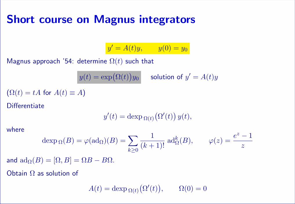
Short course on Magnus integrators

y′ = A(t)y, y(0) = y0

Magnus approach ’54: determine Ω(t) such that

y(t) = exp(Ω(t)

)y0 solution of y′ = A(t)y

(Ω(t) = tA for A(t) ≡ A)

Differentiate

y′(t) = dexp Ω(t)

(Ω′(t)

)y(t),

where

dexp Ω(B) = ϕ(adΩ)(B) =∑k≥0

1(k + 1)!

adkΩ(B), ϕ(z) =ez − 1z

and adΩ(B) = [Ω, B] = ΩB −BΩ.

Obtain Ω as solution of

A(t) = dexp Ω(t)

(Ω′(t)

), Ω(0) = 0

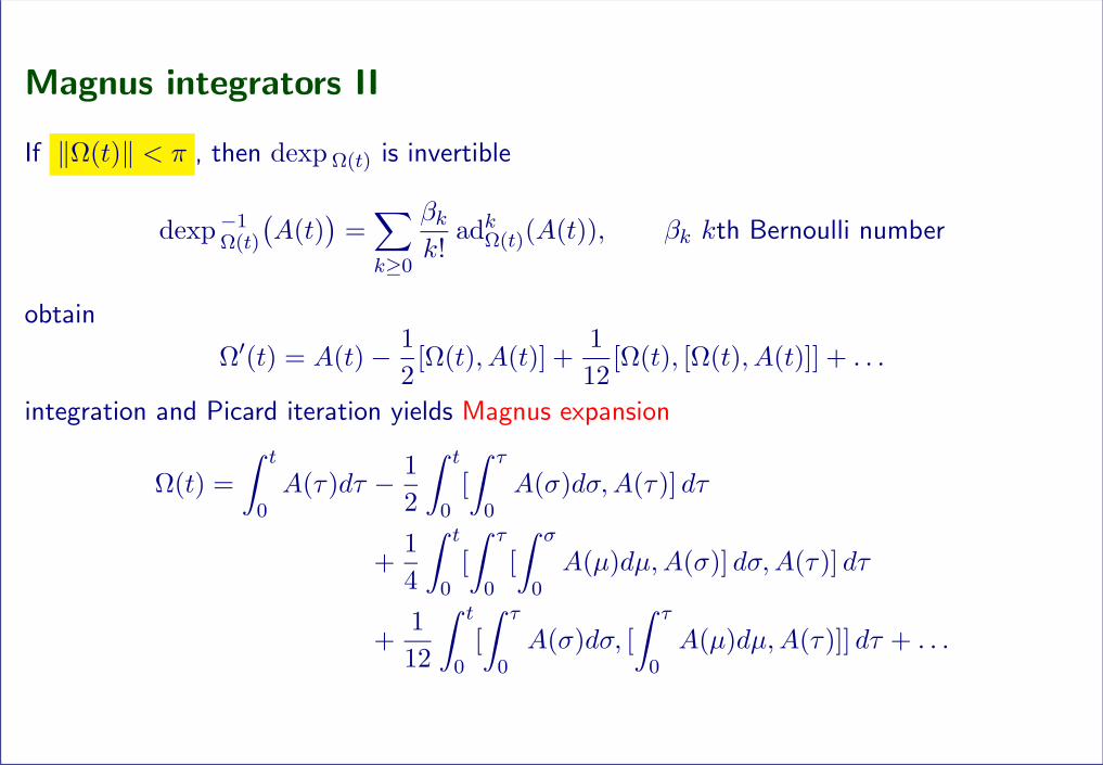
Magnus integrators II

If ‖Ω(t)‖ < π , then dexp Ω(t) is invertible

dexp−1Ω(t)

(A(t)

)=∑k≥0

βkk!

adkΩ(t)(A(t)), βk kth Bernoulli number

obtain

Ω′(t) = A(t)− 12

[Ω(t), A(t)] +112

[Ω(t), [Ω(t), A(t)]] + . . .

integration and Picard iteration yields Magnus expansion

Ω(t) =∫ t

0A(τ)dτ − 1

2

∫ t

0[∫ τ

0A(σ)dσ,A(τ)] dτ

+14

∫ t

0[∫ τ

0[∫ σ

0A(µ)dµ,A(σ)] dσ,A(τ)] dτ

+112

∫ t

0[∫ τ

0A(σ)dσ, [

∫ τ

0A(µ)dµ,A(τ)]] dτ + . . .

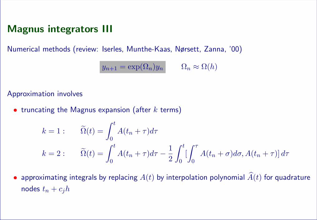
Magnus integrators III

Numerical methods (review: Iserles, Munthe-Kaas, Nørsett, Zanna, ’00)

yn+1 = exp(Ωn)yn Ωn ≈ Ω(h)

Approximation involves

• truncating the Magnus expansion (after k terms)

k = 1 : Ω(t) =∫ t

0A(tn + τ)dτ

k = 2 : Ω(t) =∫ t

0A(tn + τ)dτ − 1

2

∫ t

0[∫ τ

0A(tn + σ)dσ,A(tn + τ)] dτ

• approximating integrals by replacing A(t) by interpolation polynomial A(t) for quadrature

nodes tn + cjh

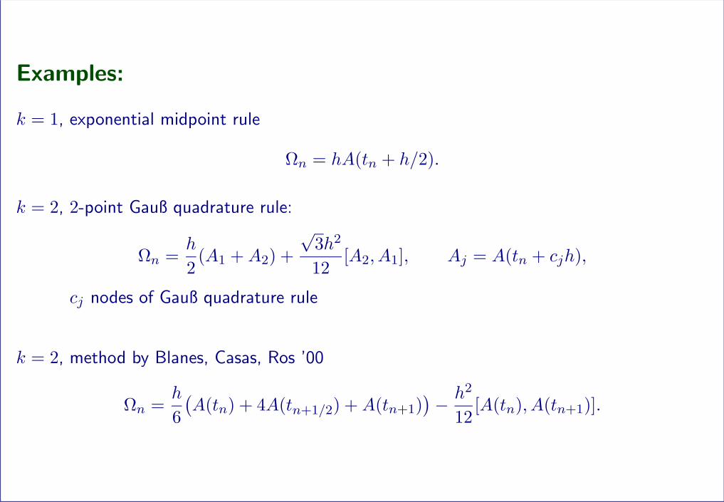
Examples:

k = 1, exponential midpoint rule

Ωn = hA(tn + h/2).

k = 2, 2-point Gauß quadrature rule:

Ωn =h

2(A1 +A2) +

√3h2

12[A2, A1], Aj = A(tn + cjh),

cj nodes of Gauß quadrature rule

k = 2, method by Blanes, Casas, Ros ’00

Ωn =h

6(A(tn) + 4A(tn+1/2) +A(tn+1)

)− h2

12[A(tn), A(tn+1)].

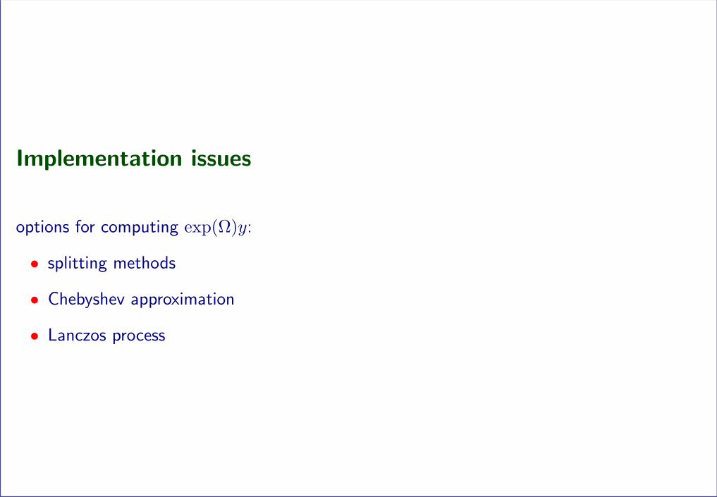
Implementation issues

options for computing exp(Ω)y:

• splitting methods

• Chebyshev approximation

• Lanczos process

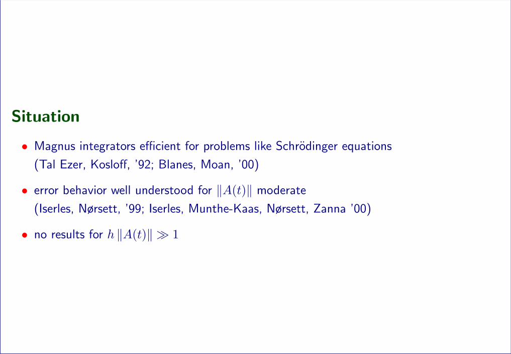
Situation

• Magnus integrators efficient for problems like Schrodinger equations

(Tal Ezer, Kosloff, ’92; Blanes, Moan, ’00)

• error behavior well understood for ‖A(t)‖ moderate

(Iserles, Nørsett, ’99; Iserles, Munthe-Kaas, Nørsett, Zanna ’00)

• no results for h ‖A(t)‖ 1

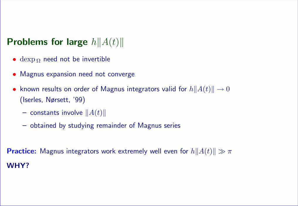
Problems for large h‖A(t)‖• dexp Ω need not be invertible

• Magnus expansion need not converge

• known results on order of Magnus integrators valid for h‖A(t)‖ → 0(Iserles, Nørsett, ’99)

– constants involve ‖A(t)‖

– obtained by studying remainder of Magnus series

Practice: Magnus integrators work extremely well even for h‖A(t)‖ π

WHY?

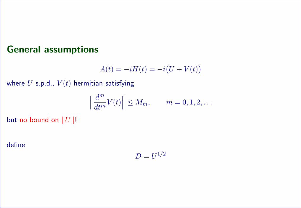
General assumptions

A(t) = −iH(t) = −i(U + V (t)

)where U s.p.d., V (t) hermitian satisfying∥∥∥ dm

dtmV (t)

∥∥∥ ≤Mm, m = 0, 1, 2, . . .

but no bound on ‖U‖!

define

D = U1/2

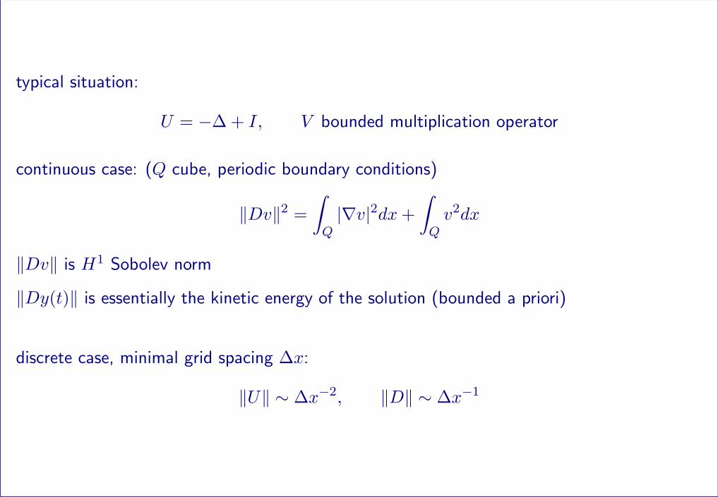
typical situation:

U = −∆ + I, V bounded multiplication operator

continuous case: (Q cube, periodic boundary conditions)

‖Dv‖2 =∫Q|∇v|2dx+

∫Qv2dx

‖Dv‖ is H1 Sobolev norm

‖Dy(t)‖ is essentially the kinetic energy of the solution (bounded a priori)

discrete case, minimal grid spacing ∆x:

‖U‖ ∼ ∆x−2, ‖D‖ ∼ ∆x−1

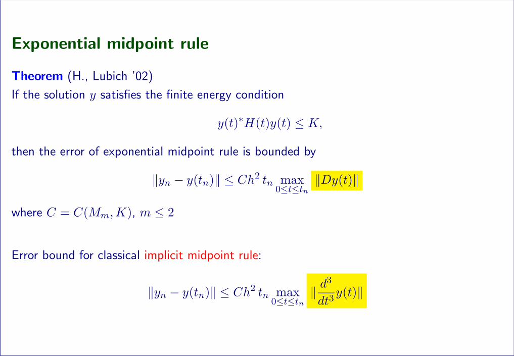
Exponential midpoint rule

Theorem (H., Lubich ’02)

If the solution y satisfies the finite energy condition

y(t)∗H(t)y(t) ≤ K,

then the error of exponential midpoint rule is bounded by

‖yn − y(tn)‖ ≤ Ch2 tn max0≤t≤tn

‖Dy(t)‖

where C = C(Mm,K), m ≤ 2

Error bound for classical implicit midpoint rule:

‖yn − y(tn)‖ ≤ Ch2 tn max0≤t≤tn

‖ d3

dt3y(t)‖

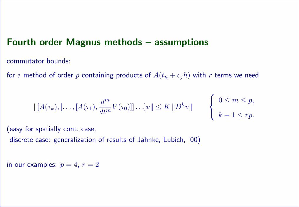
Fourth order Magnus methods – assumptions

commutator bounds:

for a method of order p containing products of A(tn + cjh) with r terms we need

‖[A(τk), [. . . , [A(τ1),dm

dtmV (τ0)]] . . .]v‖ ≤ K ‖Dkv‖

0 ≤ m ≤ p,

k + 1 ≤ rp.

(easy for spatially cont. case,

discrete case: generalization of results of Jahnke, Lubich, ’00)

in our examples: p = 4, r = 2

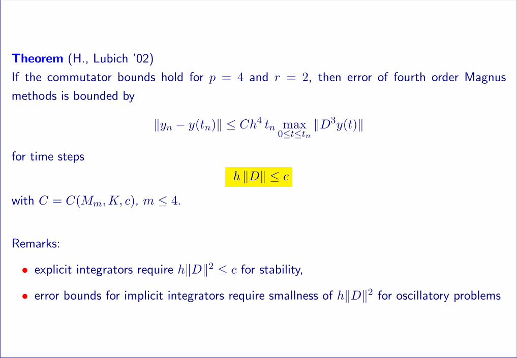
Theorem (H., Lubich ’02)

If the commutator bounds hold for p = 4 and r = 2, then error of fourth order Magnus

methods is bounded by

‖yn − y(tn)‖ ≤ Ch4 tn max0≤t≤tn

‖D3y(t)‖

for time steps

h ‖D‖ ≤ c

with C = C(Mm,K, c), m ≤ 4.

Remarks:

• explicit integrators require h‖D‖2 ≤ c for stability,

• error bounds for implicit integrators require smallness of h‖D‖2 for oscillatory problems

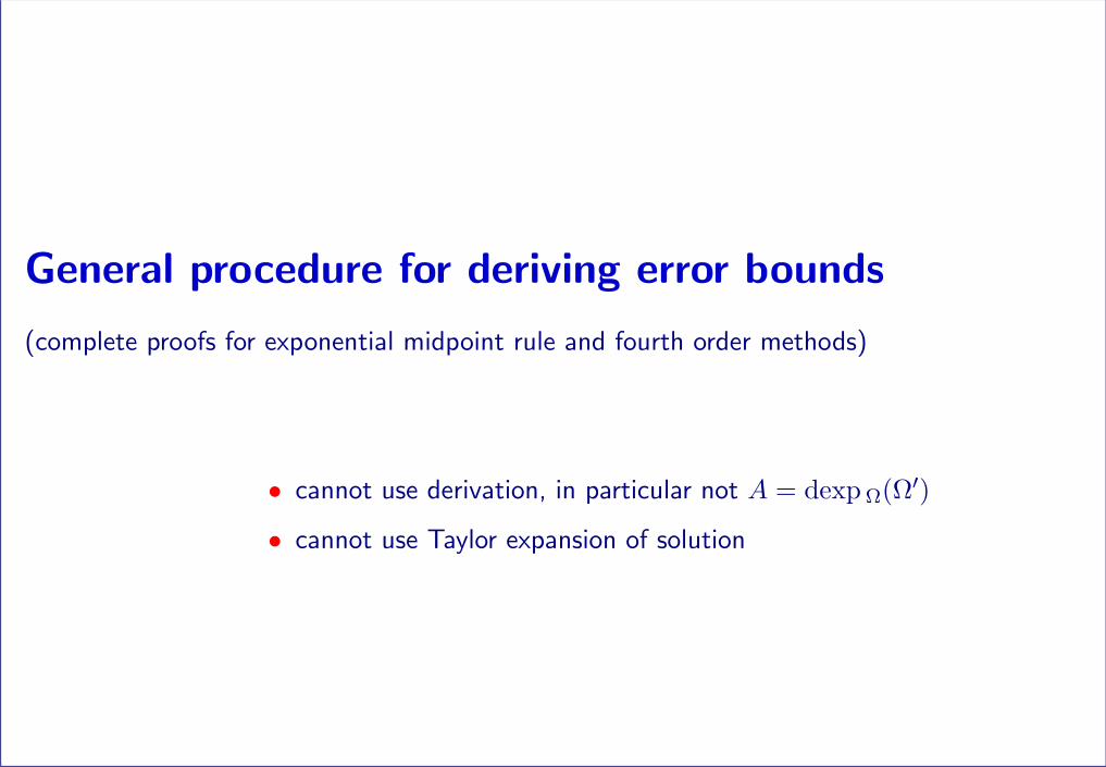
General procedure for deriving error bounds

(complete proofs for exponential midpoint rule and fourth order methods)

• cannot use derivation, in particular not A = dexp Ω(Ω′)

• cannot use Taylor expansion of solution

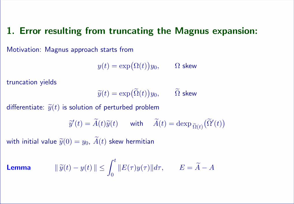
1. Error resulting from truncating the Magnus expansion:

Motivation: Magnus approach starts from

y(t) = exp(Ω(t)

)y0, Ω skew

truncation yields

y(t) = exp(Ω(t)

)y0, Ω skew

differentiate: y(t) is solution of perturbed problem

y′(t) = A(t)y(t) with A(t) = dexpΩ(t)

(Ω′(t)

)with initial value y(0) = y0, A(t) skew hermitian

Lemma ‖ y(t)− y(t) ‖ ≤∫ t

0‖E(τ)y(τ)‖dτ , E = A−A

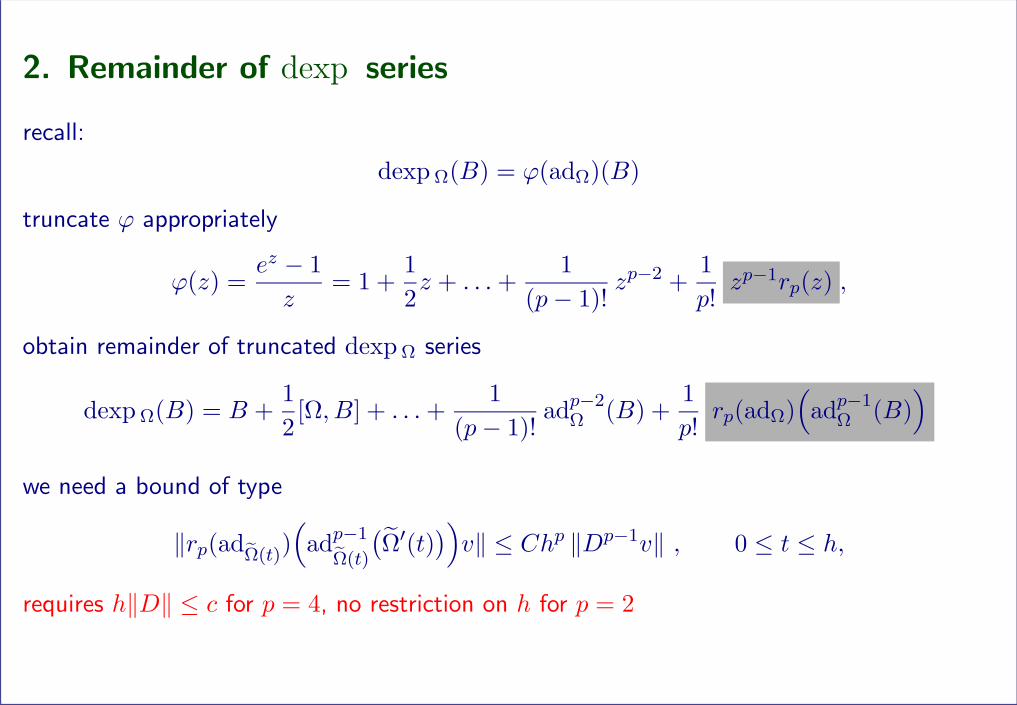
2. Remainder of dexp series

recall:

dexp Ω(B) = ϕ(adΩ)(B)

truncate ϕ appropriately

ϕ(z) =ez − 1z

= 1 +12z + . . .+

1(p− 1)!

zp−2 +1p!

zp−1rp(z) ,

obtain remainder of truncated dexp Ω series

dexp Ω(B) = B +12

[Ω, B] + . . .+1

(p− 1)!adp−2

Ω (B) +1p!

rp(adΩ)(

adp−1Ω (B)

)we need a bound of type

‖rp(adΩ(t)

)(

adp−1

Ω(t)

(Ω′(t)

))v‖ ≤ Chp ‖Dp−1v‖ , 0 ≤ t ≤ h,

requires h‖D‖ ≤ c for p = 4, no restriction on h for p = 2

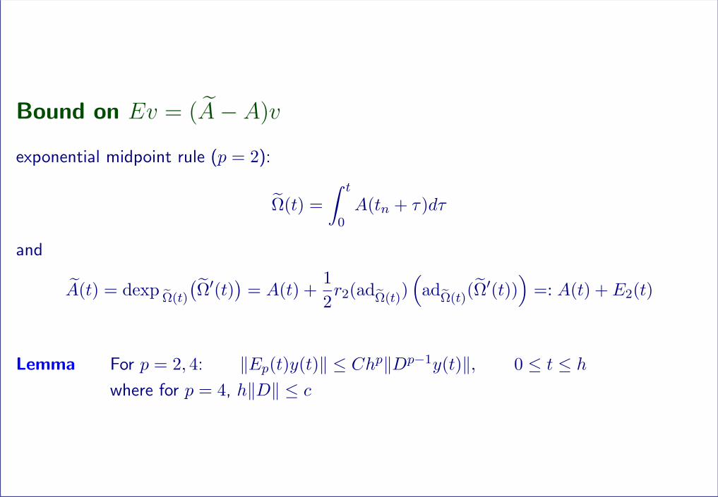
Bound on Ev = (A− A)v

exponential midpoint rule (p = 2):

Ω(t) =∫ t

0A(tn + τ)dτ

and

A(t) = dexpΩ(t)

(Ω′(t)

)= A(t) +

12r2(ad

Ω(t))(

adΩ(t)

(Ω′(t)))

=: A(t) + E2(t)

Lemma For p = 2, 4: ‖Ep(t)y(t)‖ ≤ Chp‖Dp−1y(t)‖, 0 ≤ t ≤ hwhere for p = 4, h‖D‖ ≤ c

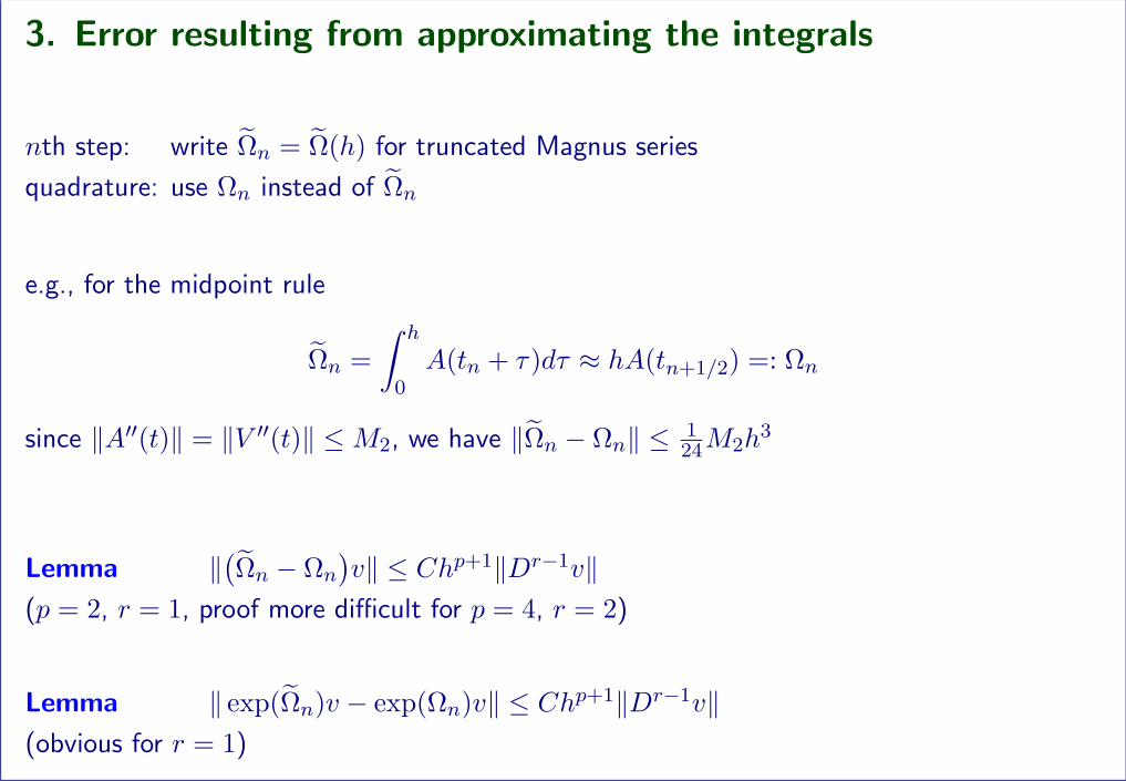
3. Error resulting from approximating the integrals

nth step: write Ωn = Ω(h) for truncated Magnus series

quadrature: use Ωn instead of Ωn

e.g., for the midpoint rule

Ωn =∫ h

0A(tn + τ)dτ ≈ hA(tn+1/2) =: Ωn

since ‖A′′(t)‖ = ‖V ′′(t)‖ ≤M2, we have ‖Ωn − Ωn‖ ≤ 124M2h

3

Lemma ‖(Ωn − Ωn

)v‖ ≤ Chp+1‖Dr−1v‖

(p = 2, r = 1, proof more difficult for p = 4, r = 2)

Lemma ‖ exp(Ωn)v − exp(Ωn)v‖ ≤ Chp+1‖Dr−1v‖(obvious for r = 1)

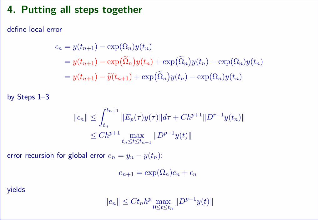
4. Putting all steps together

define local error

εn = y(tn+1)− exp(Ωn)y(tn)

= y(tn+1)− exp(Ωn

)y(tn) + exp

(Ωn

)y(tn)− exp(Ωn)y(tn)

= y(tn+1)− y(tn+1) + exp(Ωn

)y(tn)− exp(Ωn)y(tn)

by Steps 1–3

‖εn‖ ≤∫ tn+1

tn

‖Ep(τ)y(τ)‖dτ + Chp+1‖Dr−1y(tn)‖

≤ Chp+1 maxtn≤t≤tn+1

‖Dp−1y(t)‖

error recursion for global error en = yn − y(tn):

en+1 = exp(Ωn)en + εn

yields

‖en‖ ≤ Ctnhp max0≤t≤tn

‖Dp−1y(t)‖

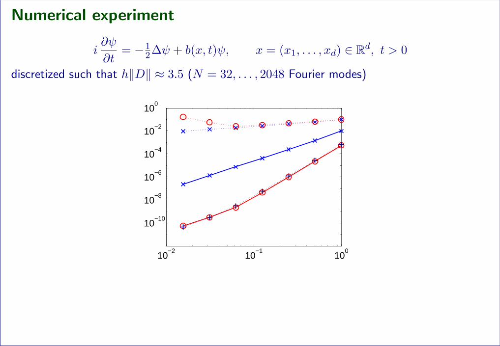
Numerical experiment

i∂ψ

∂t= −1

2∆ψ + b(x, t)ψ, x = (x1, . . . , xd) ∈ Rd, t > 0

discretized such that h‖D‖ ≈ 3.5 (N = 32, . . . , 2048 Fourier modes)

10−2

10−1

100

10−10

10−8

10−6

10−4

10−2

100

Summary

Known in practice: Magnus methods work well for time-dependent Schrodinger equations

here: theoretical explanation for this behavior, in particular

• presented optimal-order error estimates for problems where h‖H(t)‖ is large

• developed new mechanisms which lead to such bounds