OLYNOMIALS P HEBYSHEV C (I) R - McMaster Universityms.mcmaster.ca/~bprotas/MATH745a/spectr_03.pdfin...
30
Chebyshev Spectral Methods 102 C HEBYSHEV P OLYNOMIALS — R EVIEW (I) • General properties of orthogonal polynomials – Suppose I =[a, b] is a given interval. Let ϖ : I → R + be a weight function which is positive and continuous on I – Let L 2 ϖ (I ) denote the space of measurable functions v such that kvk ϖ = Z I |v(x)| 2 ϖ(x) dx 1 2 < ∞ – L 2 ϖ (I ) is a Hilbert space with the scalar products (u, v) ϖ = Z I u(x) v(x)ϖ(x) dx • Chebyshev polynomials are obtained by setting – the weight: ϖ(x)=(1 - x 2 ) - 1 2 – the interval: I =[-1, 1] – Chebyshev polynomials of degree k are expressed as T k (x)= cos(k cos -1 x), k = 0, 1, 2,...
Transcript of OLYNOMIALS P HEBYSHEV C (I) R - McMaster Universityms.mcmaster.ca/~bprotas/MATH745a/spectr_03.pdfin...
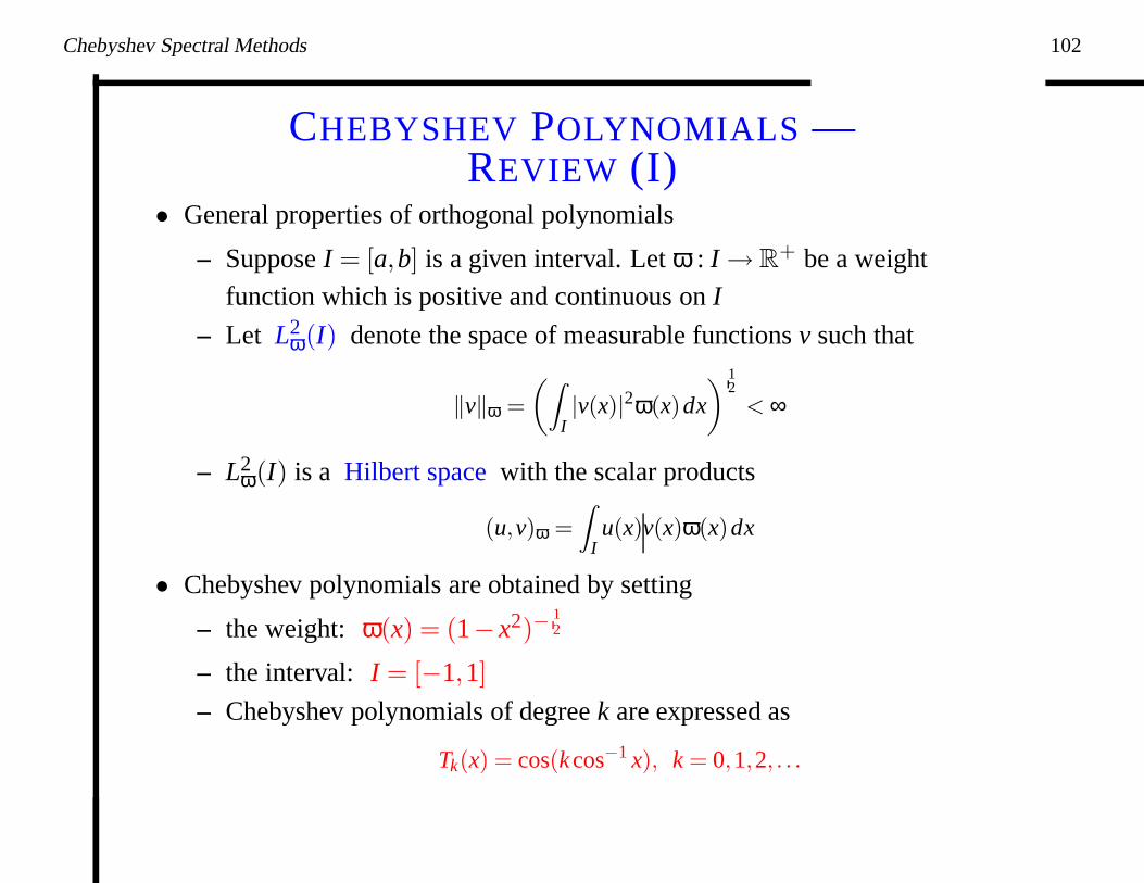
Chebyshev Spectral Methods 102
CHEBYSHEV POLYNOMIALS —REVIEW (I)
• General properties of orthogonal polynomials
– Suppose I = [a,b] is a given interval. Let ω : I → R+ be a weight
function which is positive and continuous on I
– Let L2ω(I) denote the space of measurable functions v such that
‖v‖ω =
(
Z
I|v(x)|2ω(x)dx
)12
< ∞
– L2ω(I) is a Hilbert space with the scalar products
(u,v)ω =Z
Iu(x)v(x)ω(x)dx
• Chebyshev polynomials are obtained by setting
– the weight: ω(x) = (1− x2)−12
– the interval: I = [−1,1]
– Chebyshev polynomials of degree k are expressed as
Tk(x) = cos(k cos−1 x), k = 0,1,2, . . .
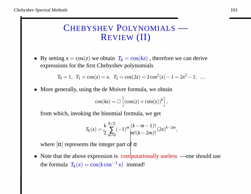
Chebyshev Spectral Methods 103
CHEBYSHEV POLYNOMIALS —REVIEW (II)
• By setting x = cos(z) we obtain Tk = cos(kz) , therefore we can deriveexpressions for the first Chebyshev polynomials
T0 = 1, T1 = cos(z) = x, T2 = cos(2z) = 2cos2(z)−1 = 2x2 −1, . . .
• More generally, using the de Moivre formula, we obtain
cos(kz) = ℜ[
(cos(z)+ isin(z))k]
,
from which, invoking the binomial formula, we get
Tk(x) =k2
[k/2]
∑m=0
(−1)m (k−m−1)!m!(k−2m)!
(2x)k−2m,
where [α] represents the integer part of α
• Note that the above expression is computationally useless — one should use
the formula Tk(x) = cos(k cos−1 x) instead!
Chebyshev Spectral Methods 104
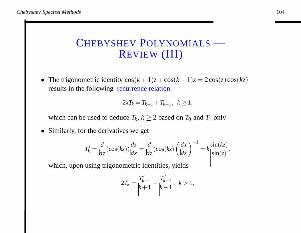
CHEBYSHEV POLYNOMIALS —REVIEW (III)
• The trigonometric identity cos(k +1)z+ cos(k−1)z = 2cos(z)cos(kz)results in the following recurrence relation
2xTk = Tk+1 +Tk−1, k ≥ 1,
which can be used to deduce Tk, k ≥ 2 based on T0 and T1 only
• Similarly, for the derivatives we get
T ′k =
ddz
(cos(kz))dzdx
=ddz
(cos(kz)
(
dxdz
)−1
= ksin(kz)sin(z)
,
which, upon using trigonometric identities, yields
2Tk =T ′
k+1
k +1−
T ′k−1
k−1, k > 1,
Chebyshev Spectral Methods 105
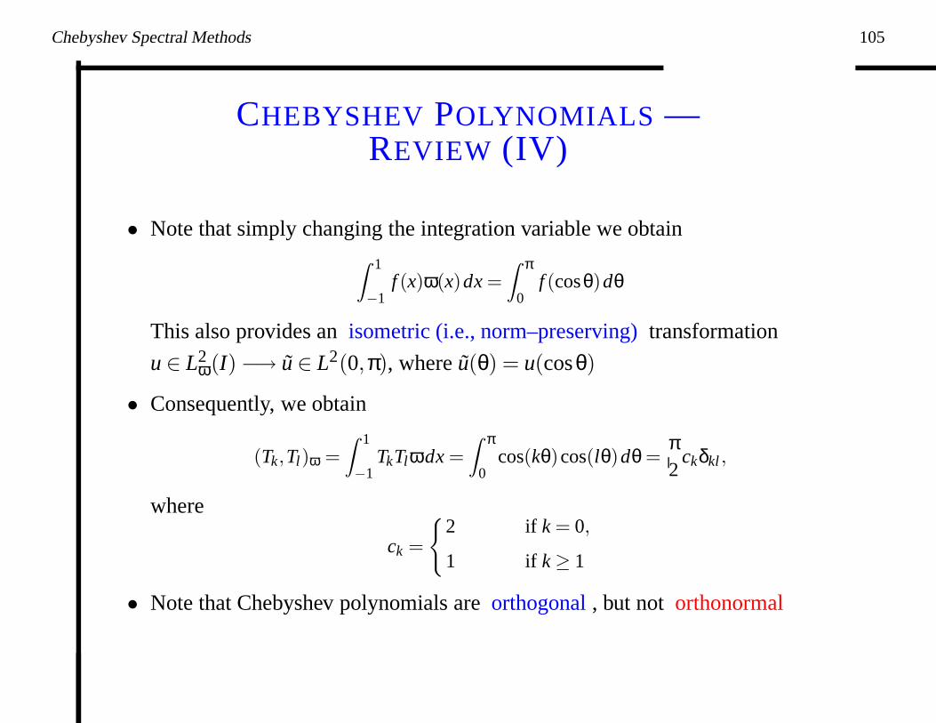
CHEBYSHEV POLYNOMIALS —REVIEW (IV)
• Note that simply changing the integration variable we obtainZ 1
−1f (x)ω(x)dx =
Z π
0f (cosθ)dθ
This also provides an isometric (i.e., norm–preserving) transformation
u ∈ L2ω(I) −→ u ∈ L2(0,π), where u(θ) = u(cosθ)
• Consequently, we obtain
(Tk,Tl)ω =
Z 1
−1TkTlωdx =
Z π
0cos(kθ)cos(lθ)dθ =
π2
ckδkl ,
where
ck =
2 if k = 0,
1 if k ≥ 1
• Note that Chebyshev polynomials are orthogonal , but not orthonormal
Chebyshev Spectral Methods 106
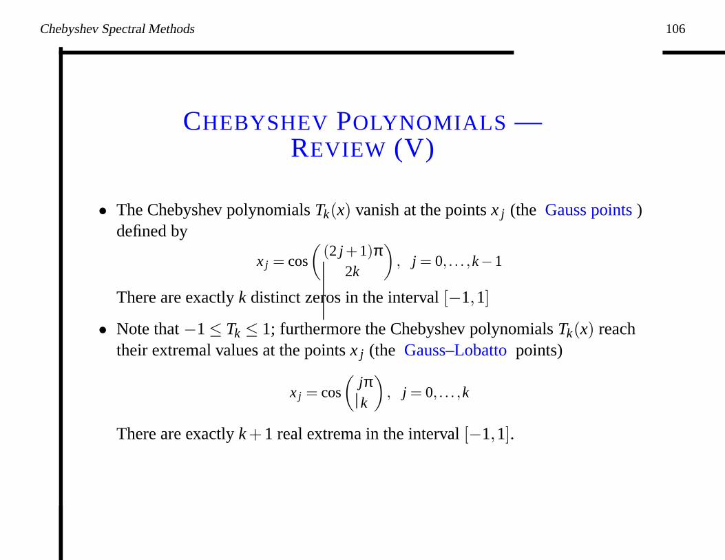
CHEBYSHEV POLYNOMIALS —REVIEW (V)
• The Chebyshev polynomials Tk(x) vanish at the points x j (the Gauss points )defined by
x j = cos
(
(2 j +1)π2k
)
, j = 0, . . . ,k−1
There are exactly k distinct zeros in the interval [−1,1]
• Note that −1 ≤ Tk ≤ 1; furthermore the Chebyshev polynomials Tk(x) reachtheir extremal values at the points x j (the Gauss–Lobatto points)
x j = cos
(
jπk
)
, j = 0, . . . ,k
There are exactly k +1 real extrema in the interval [−1,1].
Chebyshev Spectral Methods 107
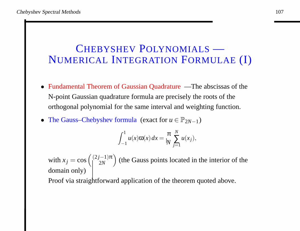
CHEBYSHEV POLYNOMIALS —NUMERICAL INTEGRATION FORMULAE (I)
• Fundamental Theorem of Gaussian Quadrature — The abscissas of the
N-point Gaussian quadrature formula are precisely the roots of the
orthogonal polynomial for the same interval and weighting function.
• The Gauss–Chebyshev formula (exact for u ∈ P2N−1)
Z 1
−1u(x)ω(x)dx =
πN
N
∑j=1
u(x j),
with x j = cos(
(2 j−1)π2N
)
(the Gauss points located in the interior of the
domain only)
Proof via straightforward application of the theorem quoted above.
Chebyshev Spectral Methods 108
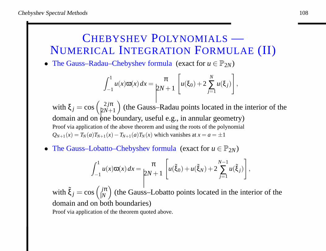
CHEBYSHEV POLYNOMIALS —NUMERICAL INTEGRATION FORMULAE (II)
• The Gauss–Radau–Chebyshev formula (exact for u ∈ P2N )
Z 1
−1u(x)ω(x)dx =
π2N +1
[
u(ξ0)+2N
∑j=1
u(ξ j)
]
,
with ξ j = cos(
2 jπ2N+1
)
(the Gauss–Radau points located in the interior of the
domain and on one boundary, useful e.g., in annular geometry)Proof via application of the above theorem and using the roots of the polynomialQN+1(x) = TN(a)TN+1(x)−TN+1(a)TN(x) which vanishes at x = a = ±1
• The Gauss–Lobatto–Chebyshev formula (exact for u ∈ P2N )
Z 1
−1u(x)ω(x)dx =
π2N +1
[
u(ξ0)+u(ξN)+2N−1
∑j=1
u(ξ j)
]
,
with ξ j = cos(
jπN
)
(the Gauss–Lobatto points located in the interior of the
domain and on both boundaries)Proof via application of the theorem quoted above.
Chebyshev Spectral Methods 109
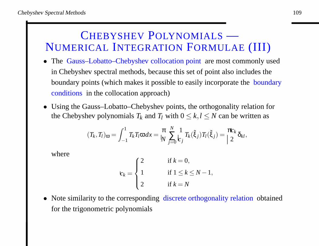
CHEBYSHEV POLYNOMIALS —NUMERICAL INTEGRATION FORMULAE (III)• The Gauss–Lobatto–Chebyshev collocation point are most commonly used
in Chebyshev spectral methods, because this set of point also includes the
boundary points (which makes it possible to easily incorporate the boundary
conditions in the collocation approach)
• Using the Gauss–Lobatto–Chebyshev points, the orthogonality relation forthe Chebyshev polynomials Tk and Tl with 0 ≤ k, l ≤ N can be written as
(Tk,Tl)ω =Z 1
−1TkTlωdx =
πN
N
∑j=0
1c j
Tk(ξ j)Tl(ξ j) =πck
2δkl ,
where
ck =
2 if k = 0,
1 if 1 ≤ k ≤ N −1,
2 if k = N
• Note similarity to the corresponding discrete orthogonality relation obtained
for the trigonometric polynomials
Chebyshev Spectral Methods 110
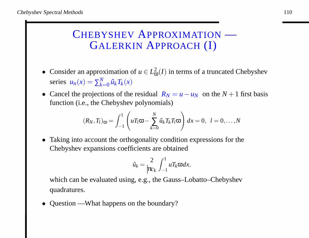
CHEBYSHEV APPROXIMATION —GALERKIN APPROACH (I)
• Consider an approximation of u ∈ L2ω(I) in terms of a truncated Chebyshev
series un(x) = ∑Nk=0 ukTk(x)
• Cancel the projections of the residual RN = u−uN on the N +1 first basisfunction (i.e., the Chebyshev polynomials)
(RN ,Tl)ω =Z 1
−1
(
uTlω−N
∑k=0
ukTkTlω
)
dx = 0, l = 0, . . . ,N
• Taking into account the orthogonality condition expressions for theChebyshev expansions coefficients are obtained
uk =2
πck
Z 1
−1uTkωdx,
which can be evaluated using, e.g., the Gauss–Lobatto–Chebyshev
quadratures.
• Question — What happens on the boundary?
Chebyshev Spectral Methods 111
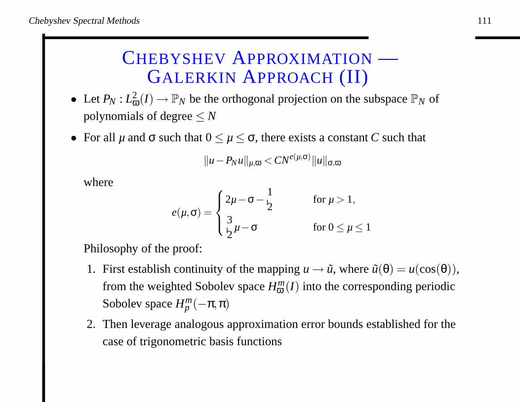
CHEBYSHEV APPROXIMATION —GALERKIN APPROACH (II)
• Let PN : L2ω(I) → PN be the orthogonal projection on the subspace PN of
polynomials of degree ≤ N
• For all µ and σ such that 0 ≤ µ ≤ σ, there exists a constant C such that
‖u−PN u‖µ,ω < CNe(µ,σ)‖u‖σ,ω
where
e(µ,σ) =
2µ−σ−12
for µ > 1,
32
µ−σ for 0 ≤ µ ≤ 1
Philosophy of the proof:
1. First establish continuity of the mapping u → u, where u(θ) = u(cos(θ)),
from the weighted Sobolev space Hmω (I) into the corresponding periodic
Sobolev space Hmp (−π,π)
2. Then leverage analogous approximation error bounds established for the
case of trigonometric basis functions
Chebyshev Spectral Methods 112
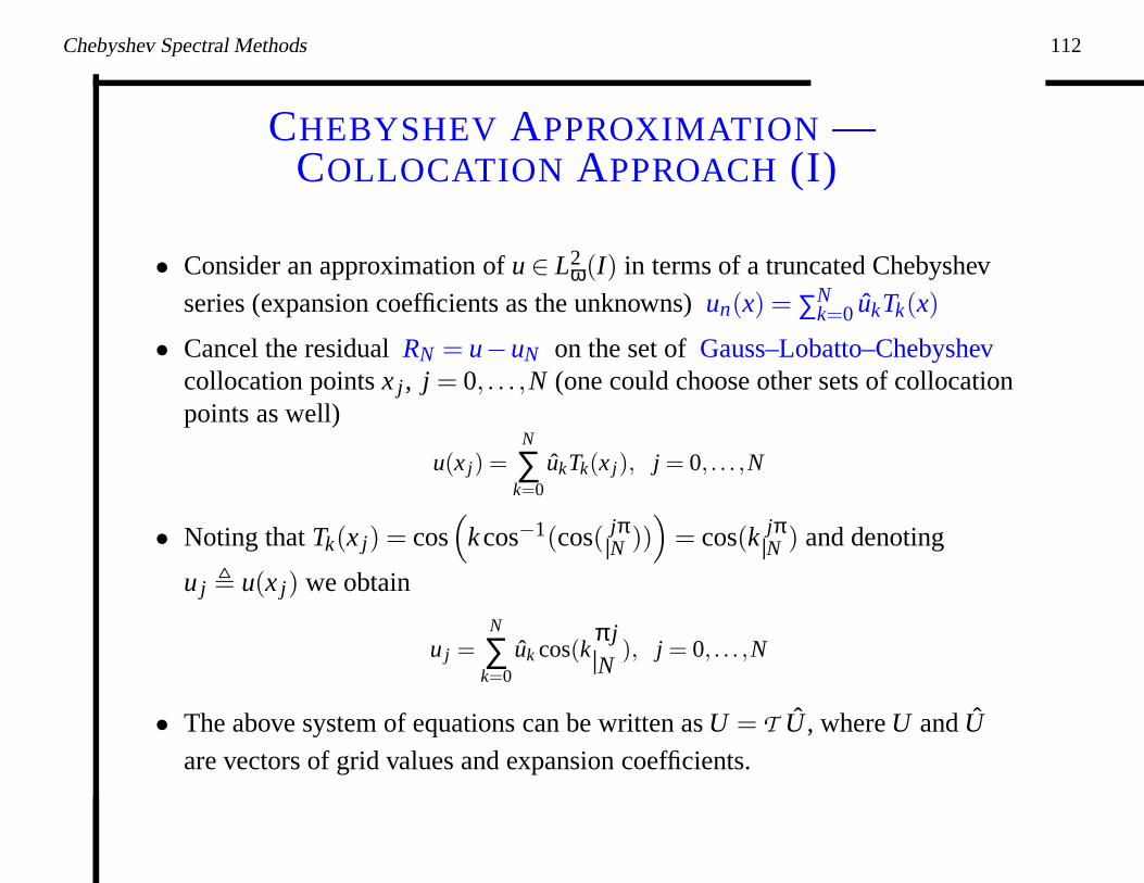
CHEBYSHEV APPROXIMATION —COLLOCATION APPROACH (I)
• Consider an approximation of u ∈ L2ω(I) in terms of a truncated Chebyshev
series (expansion coefficients as the unknowns) un(x) = ∑Nk=0 ukTk(x)
• Cancel the residual RN = u−uN on the set of Gauss–Lobatto–Chebyshevcollocation points x j, j = 0, . . . ,N (one could choose other sets of collocationpoints as well)
u(x j) =N
∑k=0
ukTk(x j), j = 0, . . . ,N
• Noting that Tk(x j) = cos(
k cos−1(cos( jπN )))
= cos(k jπN ) and denoting
u j , u(x j) we obtain
u j =N
∑k=0
uk cos(kπ jN
), j = 0, . . . ,N
• The above system of equations can be written as U = T U , where U and U
are vectors of grid values and expansion coefficients.
Chebyshev Spectral Methods 113
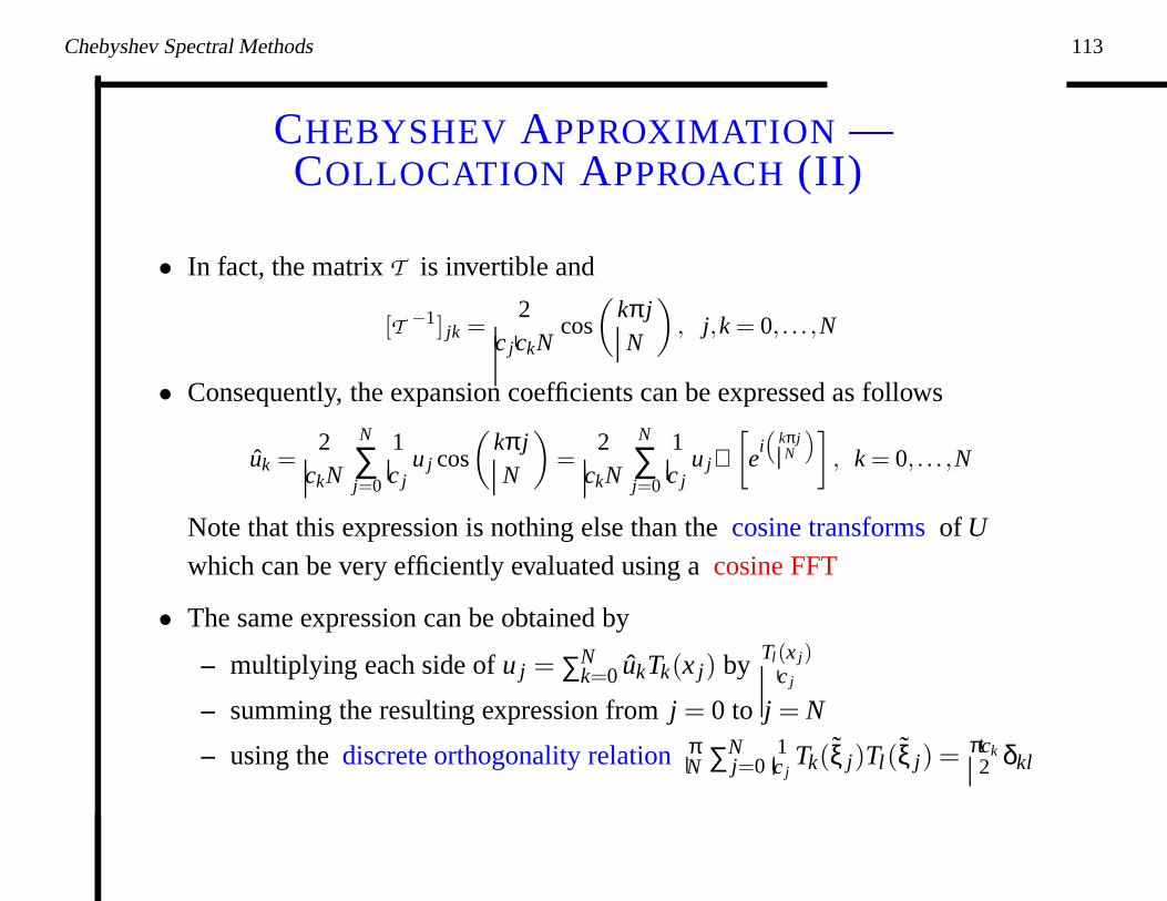
CHEBYSHEV APPROXIMATION —COLLOCATION APPROACH (II)
• In fact, the matrix T is invertible and
[T −1] jk =2
c jckNcos
(
kπ jN
)
, j,k = 0, . . . ,N
• Consequently, the expansion coefficients can be expressed as follows
uk =2
ckN
N
∑j=0
1c j
u j cos
(
kπ jN
)
=2
ckN
N
∑j=0
1c j
u jℜ[
ei(
kπ jN
)]
, k = 0, . . . ,N
Note that this expression is nothing else than the cosine transforms of U
which can be very efficiently evaluated using a cosine FFT
• The same expression can be obtained by
– multiplying each side of u j = ∑Nk=0 ukTk(x j) by Tl(x j)
c j
– summing the resulting expression from j = 0 to j = N
– using the discrete orthogonality relation πN ∑N
j=01c j
Tk(ξ j)Tl(ξ j) = πck2 δkl
Chebyshev Spectral Methods 114
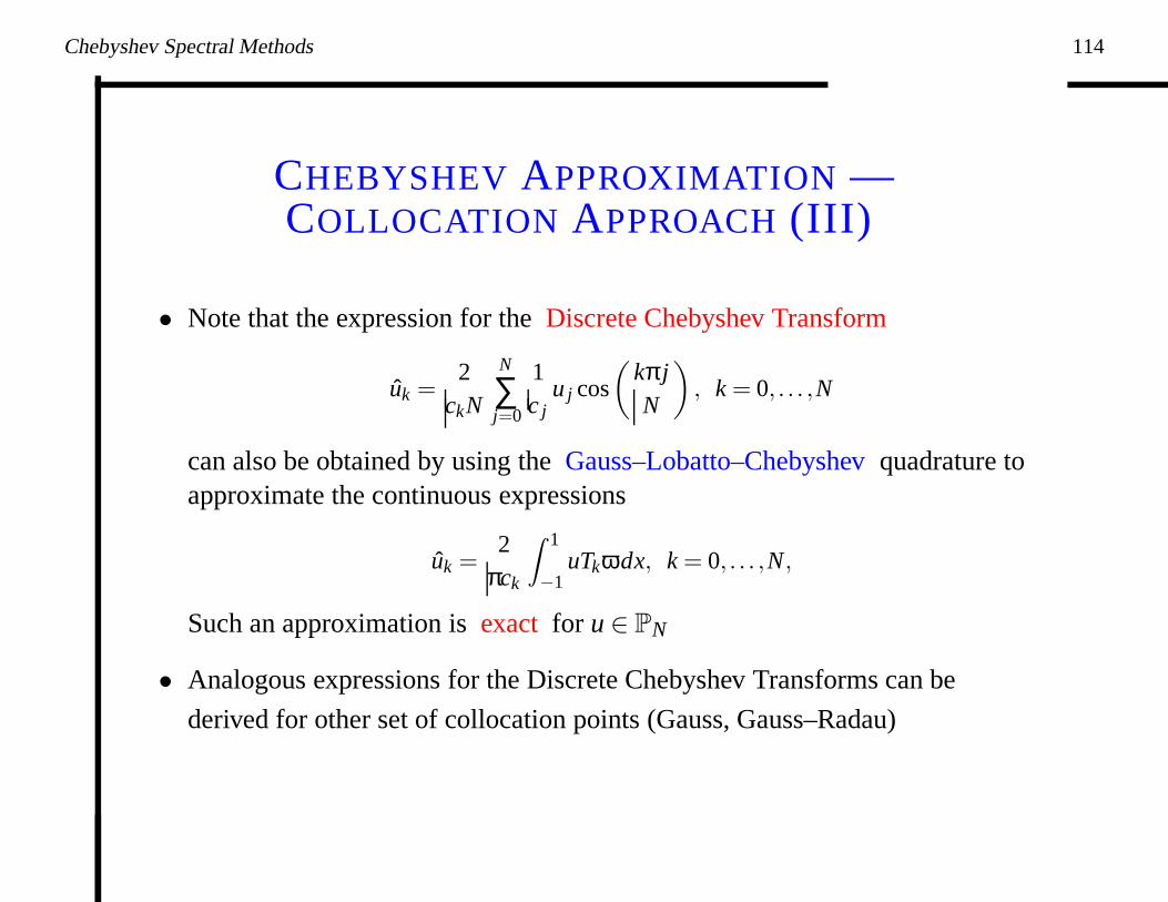
CHEBYSHEV APPROXIMATION —COLLOCATION APPROACH (III)
• Note that the expression for the Discrete Chebyshev Transform
uk =2
ckN
N
∑j=0
1c j
u j cos
(
kπ jN
)
, k = 0, . . . ,N
can also be obtained by using the Gauss–Lobatto–Chebyshev quadrature toapproximate the continuous expressions
uk =2
πck
Z 1
−1uTkωdx, k = 0, . . . ,N,
Such an approximation is exact for u ∈ PN
• Analogous expressions for the Discrete Chebyshev Transforms can be
derived for other set of collocation points (Gauss, Gauss–Radau)
Chebyshev Spectral Methods 115
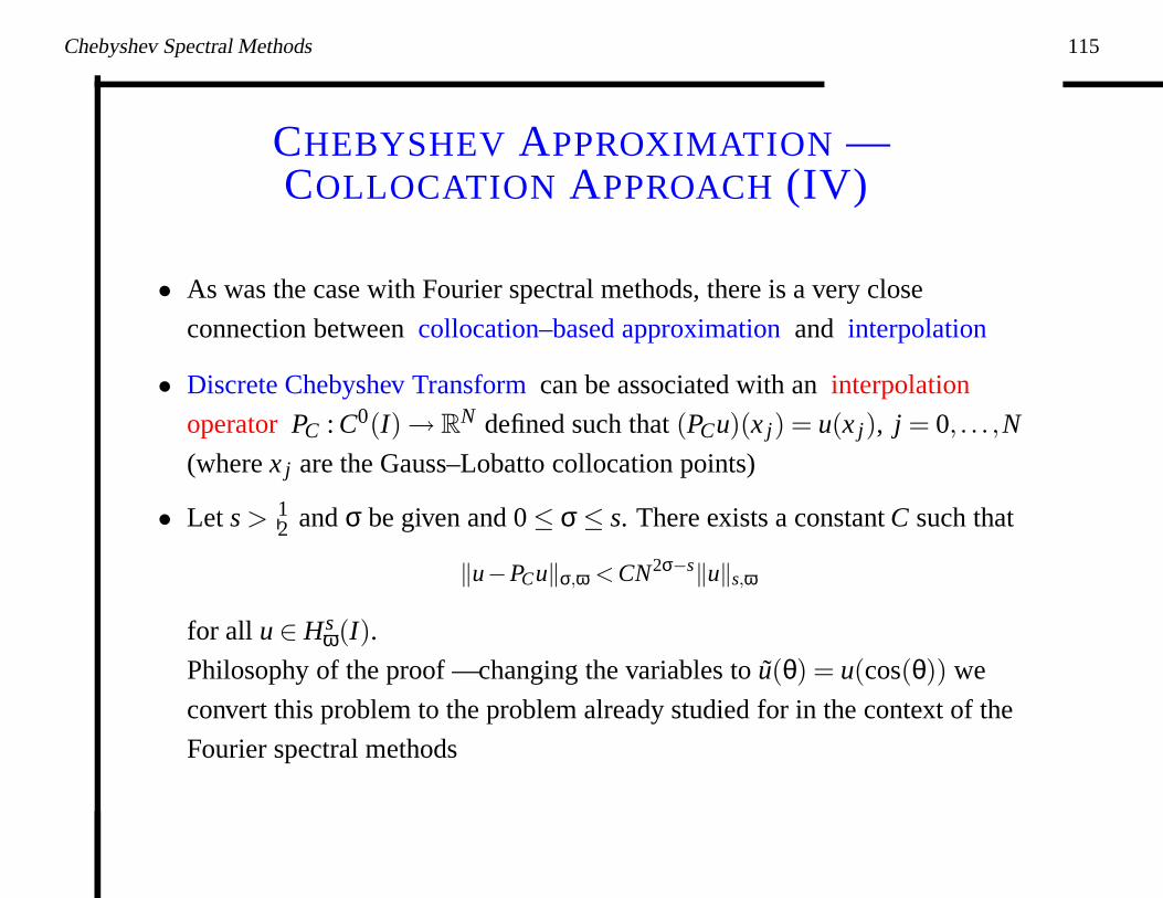
CHEBYSHEV APPROXIMATION —COLLOCATION APPROACH (IV)
• As was the case with Fourier spectral methods, there is a very close
connection between collocation–based approximation and interpolation
• Discrete Chebyshev Transform can be associated with an interpolation
operator PC : C0(I) → RN defined such that (PCu)(x j) = u(x j), j = 0, . . . ,N
(where x j are the Gauss–Lobatto collocation points)
• Let s > 12 and σ be given and 0 ≤ σ ≤ s. There exists a constant C such that
‖u−PCu‖σ,ω < CN2σ−s‖u‖s,ω
for all u ∈ Hsω(I).
Philosophy of the proof — changing the variables to u(θ) = u(cos(θ)) we
convert this problem to the problem already studied for in the context of the
Fourier spectral methods
Chebyshev Spectral Methods 116
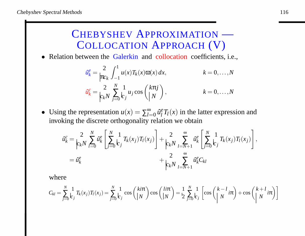
CHEBYSHEV APPROXIMATION —COLLOCATION APPROACH (V)
• Relation between the Galerkin and collocation coefficients, i.e.,
uek =
2πck
Z 1
−1u(x)Tk(x)ω(x)dx, k = 0, . . . ,N
uck =
2ckN
N
∑j=0
1c j
u j cos
(
kπ jN
)
, k = 0, . . . ,N
• Using the representation u(x) = ∑∞l=0 ue
l Tl(x) in the latter expression andinvoking the discrete orthogonality relation we obtain
uck =
2ckN
N
∑l=0
uek
[
N
∑j=0
1c j
Tk(x j)Tl(x j)
]
+2
ckN
∞
∑l=N+1
uek
[
N
∑j=0
1c j
Tk(x j)Tl(x j)
]
,
= uek +
2ckN
∞
∑l=N+1
uekCkl
where
Ckl =N
∑j=0
1c j
Tk(x j)Tl(x j)=N
∑j=0
1c j
cos
(
kiπN
)
cos
(
liπN
)
=12
N
∑j=0
1c j
[
cos
(
k− lN
iπ)
+ cos
(
k + lN
iπ)]
Chebyshev Spectral Methods 117
CHEBYSHEV APPROXIMATION —COLLOCATION APPROACH (VI)
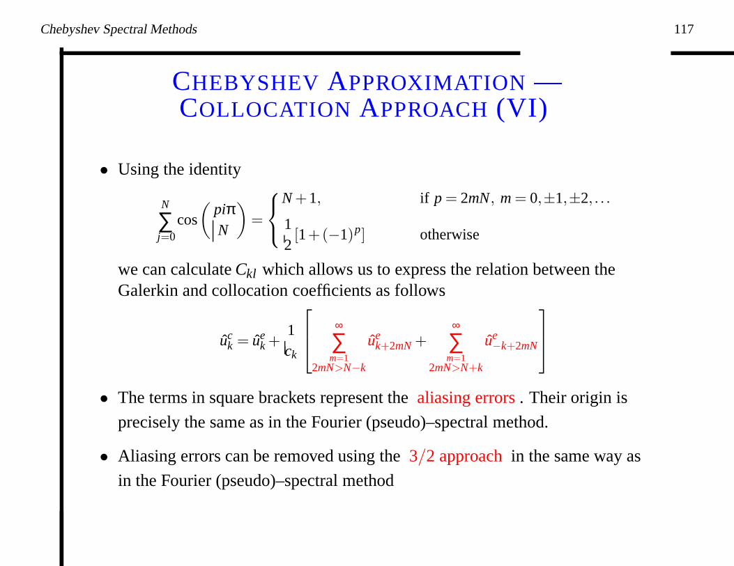
• Using the identity
N
∑j=0
cos
(
piπN
)
=
N +1, if p = 2mN, m = 0,±1,±2, . . .
12[1+(−1)p] otherwise
we can calculate Ckl which allows us to express the relation between theGalerkin and collocation coefficients as follows
uck = ue
k +1ck
∞
∑m=1
2mN>N−k
uek+2mN +
∞
∑m=1
2mN>N+k
ue−k+2mN
• The terms in square brackets represent the aliasing errors . Their origin is
precisely the same as in the Fourier (pseudo)–spectral method.
• Aliasing errors can be removed using the 3/2 approach in the same way as
in the Fourier (pseudo)–spectral method
Chebyshev Spectral Methods 118
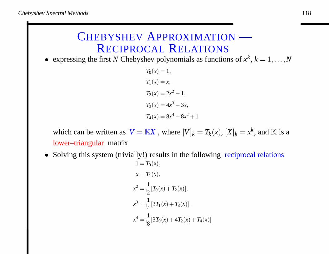
CHEBYSHEV APPROXIMATION —RECIPROCAL RELATIONS
• expressing the first N Chebyshev polynomials as functions of xk, k = 1, . . . ,N
T0(x) = 1,
T1(x) = x,
T2(x) = 2x2 −1,
T3(x) = 4x3 −3x,
T4(x) = 8x4 −8x2 +1
which can be written as V = KX , where [V ]k = Tk(x), [X ]k = xk, and K is a
lower–triangular matrix
• Solving this system (trivially!) results in the following reciprocal relations1 = T0(x),
x = T1(x),
x2 =12
[T0(x)+T2(x)],
x3 =14
[3T1(x)+T3(x)],
x4 =18
[3T0(x)+4T2(x)+T4(x)]
Chebyshev Spectral Methods 119
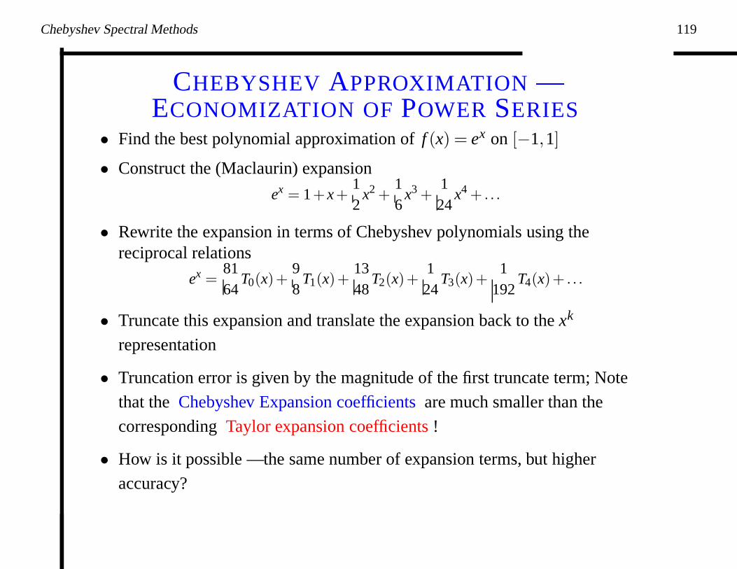
CHEBYSHEV APPROXIMATION —ECONOMIZATION OF POWER SERIES
• Find the best polynomial approximation of f (x) = ex on [−1,1]
• Construct the (Maclaurin) expansion
ex = 1+ x+12
x2 +16
x3 +124
x4 + . . .
• Rewrite the expansion in terms of Chebyshev polynomials using thereciprocal relations
ex =8164
T0(x)+98
T1(x)+1348
T2(x)+124
T3(x)+1
192T4(x)+ . . .
• Truncate this expansion and translate the expansion back to the xk
representation
• Truncation error is given by the magnitude of the first truncate term; Note
that the Chebyshev Expansion coefficients are much smaller than the
corresponding Taylor expansion coefficients !
• How is it possible — the same number of expansion terms, but higher
accuracy?
Chebyshev Spectral Methods 120
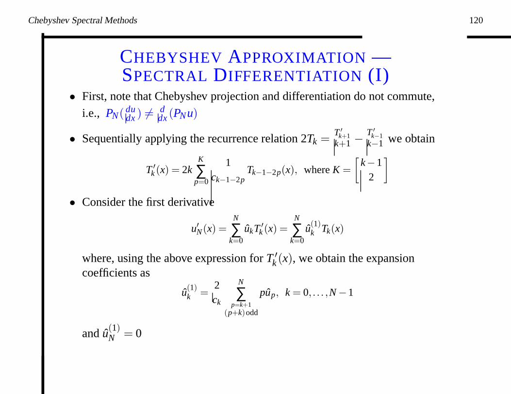
CHEBYSHEV APPROXIMATION —SPECTRAL DIFFERENTIATION (I)
• First, note that Chebyshev projection and differentiation do not commute,
i.e., PN( dudx ) 6= d
dx (PNu)
• Sequentially applying the recurrence relation 2Tk =T ′
k+1k+1 −
T ′k−1
k−1 we obtain
T ′k (x) = 2k
K
∑p=0
1ck−1−2p
Tk−1−2p(x), where K =
[
k−12
]
• Consider the first derivative
u′N(x) =N
∑k=0
ukT ′k (x) =
N
∑k=0
u(1)k Tk(x)
where, using the above expression for T ′k (x), we obtain the expansion
coefficients as
u(1)k =
2ck
N
∑p=k+1
(p+k)odd
pup, k = 0, . . . ,N −1
and u(1)N = 0
Chebyshev Spectral Methods 121
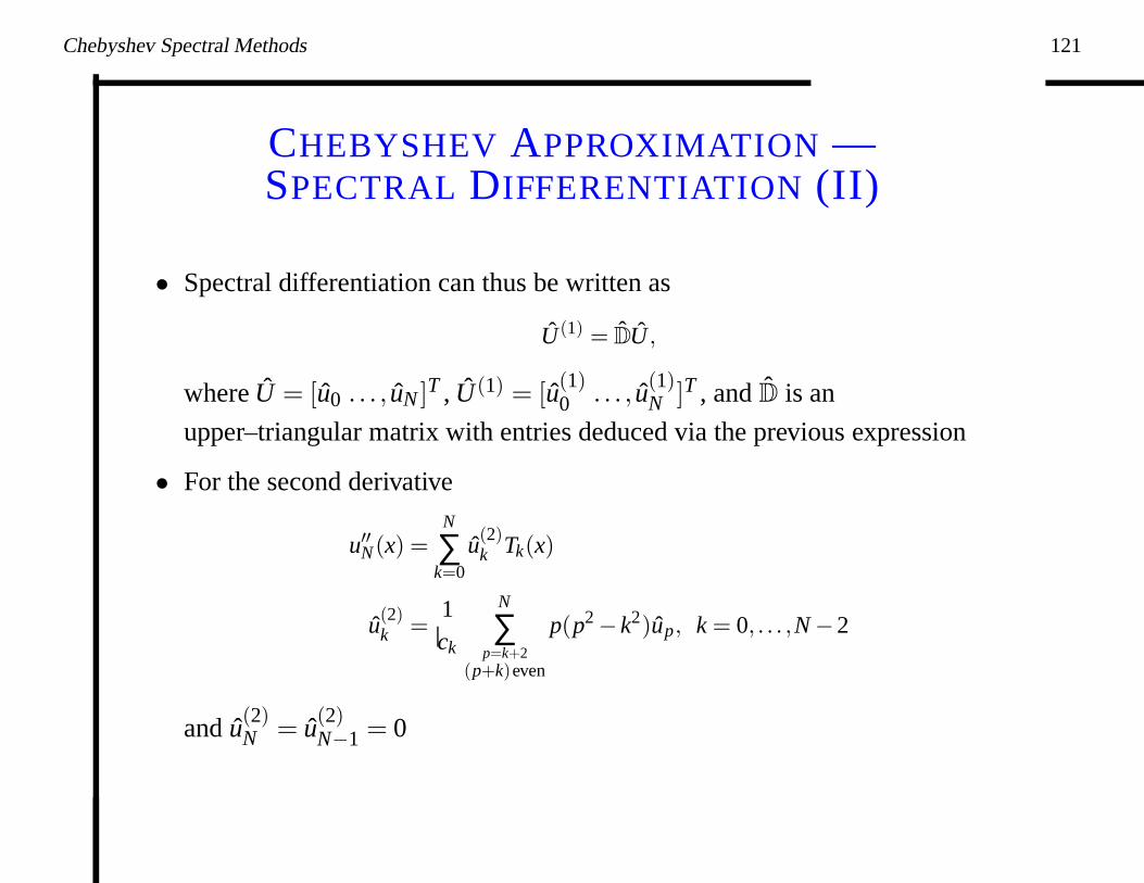
CHEBYSHEV APPROXIMATION —SPECTRAL DIFFERENTIATION (II)
• Spectral differentiation can thus be written as
U (1) = DU ,
where U = [u0 . . . , uN ]T , U (1) = [u(1)0 . . . , u(1)
N ]T , and D is an
upper–triangular matrix with entries deduced via the previous expression
• For the second derivative
u′′N(x) =N
∑k=0
u(2)k Tk(x)
u(2)k =
1ck
N
∑p=k+2
(p+k)even
p(p2 − k2)up, k = 0, . . . ,N −2
and u(2)N = u(2)
N−1 = 0
Chebyshev Spectral Methods 122
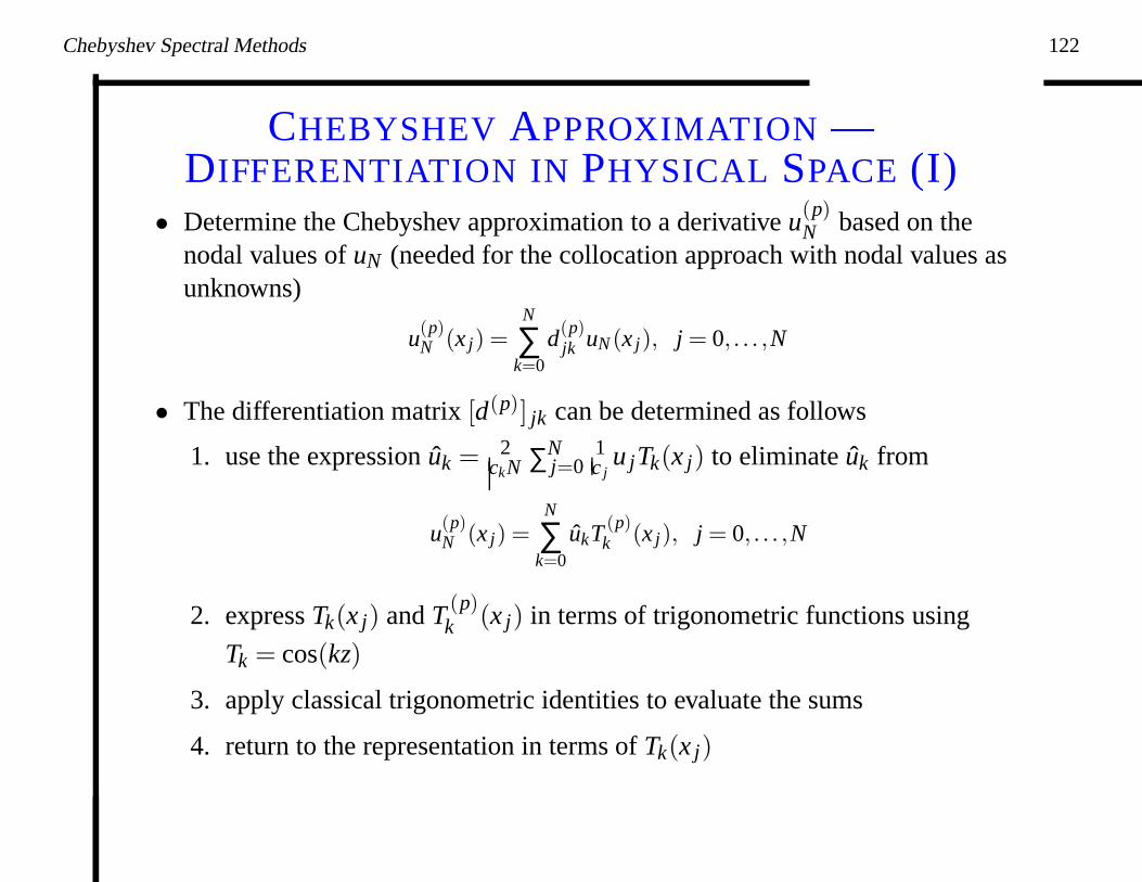
CHEBYSHEV APPROXIMATION —DIFFERENTIATION IN PHYSICAL SPACE (I)
• Determine the Chebyshev approximation to a derivative u(p)N based on the
nodal values of uN (needed for the collocation approach with nodal values asunknowns)
u(p)N (x j) =
N
∑k=0
d(p)jk uN(x j), j = 0, . . . ,N
• The differentiation matrix [d(p)] jk can be determined as follows
1. use the expression uk = 2ckN ∑N
j=01c j
u jTk(x j) to eliminate uk from
u(p)N (x j) =
N
∑k=0
ukT (p)k (x j), j = 0, . . . ,N
2. express Tk(x j) and T (p)k (x j) in terms of trigonometric functions using
Tk = cos(kz)
3. apply classical trigonometric identities to evaluate the sums
4. return to the representation in terms of Tk(x j)

Chebyshev Spectral Methods 123
CHEBYSHEV APPROXIMATION —DIFFERENTIATION IN PHYSICAL SPACE (II)
• Expressions for the entries of d(1)jk at the the Gauss–Lobatto–Chebyshev
collocation points
d(1)jk =
c j
ck
(−1) j+k
x j − xk, 0 ≤ j,k ≤ N, j 6= k,
d(1)j j = −
x j
2(1− x2j )
, 1 ≤ j ≤ N −1,
d(1)00 = −d(1)
NN =2N2 +1
6,
• ThusU (1) = DU
Chebyshev Spectral Methods 124
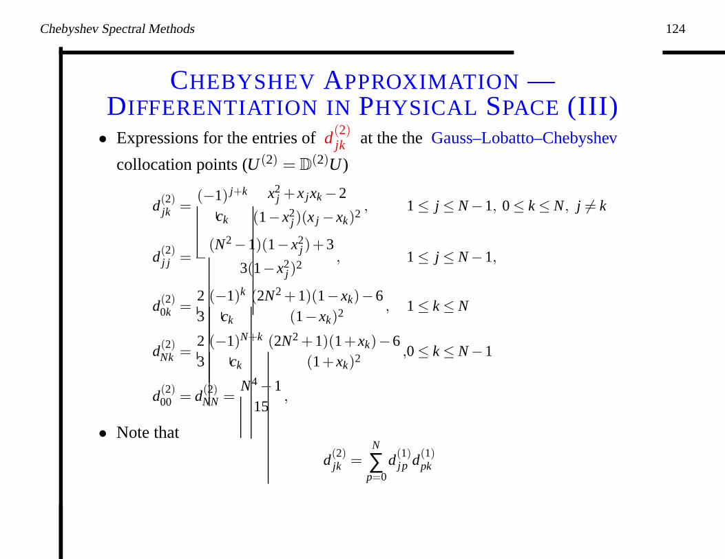
CHEBYSHEV APPROXIMATION —DIFFERENTIATION IN PHYSICAL SPACE (III)• Expressions for the entries of d(2)
jk at the the Gauss–Lobatto–Chebyshev
collocation points (U (2) = D(2)U)
d(2)jk =
(−1) j+k
ck
x2j + x jxk −2
(1− x2j)(x j − xk)2
, 1 ≤ j ≤ N −1, 0 ≤ k ≤ N, j 6= k
d(2)j j = −
(N2 −1)(1− x2j)+3
3(1− x2j )
2, 1 ≤ j ≤ N −1,
d(2)0k =
23
(−1)k
ck
(2N2 +1)(1− xk)−6(1− xk)2 , 1 ≤ k ≤ N
d(2)Nk =
23
(−1)N+k
ck
(2N2 +1)(1+ xk)−6(1+ xk)2 ,0 ≤ k ≤ N −1
d(2)00 = d(2)
NN =N4 −1
15,
• Note that
d(2)jk =
N
∑p=0
d(1)jp d(1)
pk
Chebyshev Spectral Methods 125
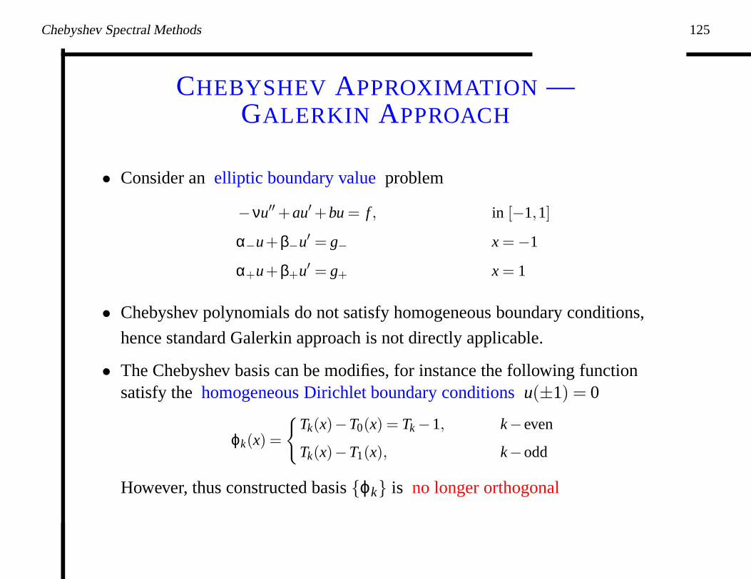
CHEBYSHEV APPROXIMATION —GALERKIN APPROACH
• Consider an elliptic boundary value problem
−νu′′ +au′ +bu = f , in [−1,1]
α−u+β−u′ = g− x = −1
α+u+β+u′ = g+ x = 1
• Chebyshev polynomials do not satisfy homogeneous boundary conditions,
hence standard Galerkin approach is not directly applicable.
• The Chebyshev basis can be modifies, for instance the following functionsatisfy the homogeneous Dirichlet boundary conditions u(±1) = 0
ϕk(x) =
Tk(x)−T0(x) = Tk −1, k− even
Tk(x)−T1(x), k−odd
However, thus constructed basis ϕk is no longer orthogonal
Chebyshev Spectral Methods 126
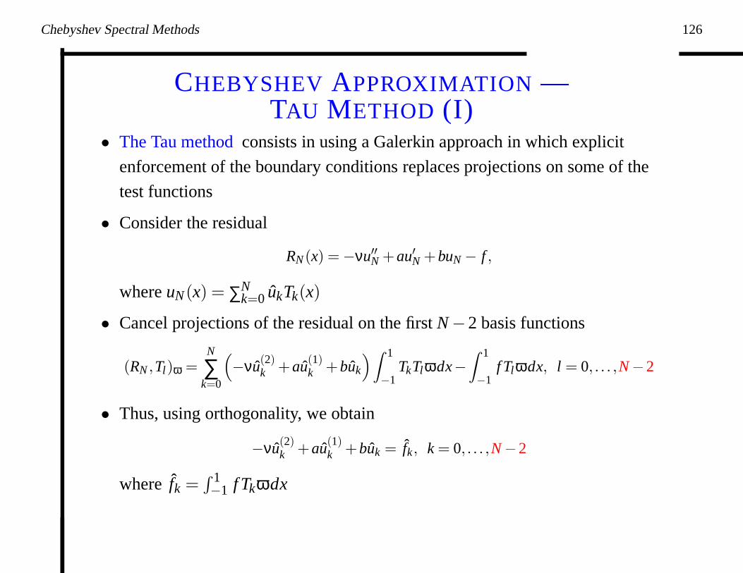
CHEBYSHEV APPROXIMATION —TAU METHOD (I)
• The Tau method consists in using a Galerkin approach in which explicit
enforcement of the boundary conditions replaces projections on some of the
test functions
• Consider the residual
RN(x) = −νu′′N +au′N +buN − f ,
where uN(x) = ∑Nk=0 ukTk(x)
• Cancel projections of the residual on the first N −2 basis functions
(RN ,Tl)ω =N
∑k=0
(
−νu(2)k +au(1)
k +buk
)
Z 1
−1TkTlωdx−
Z 1
−1f Tlωdx, l = 0, . . . ,N −2
• Thus, using orthogonality, we obtain
−νu(2)k +au(1)
k +buk = fk, k = 0, . . . ,N −2
where fk =R 1−1 f Tkωdx
Chebyshev Spectral Methods 127
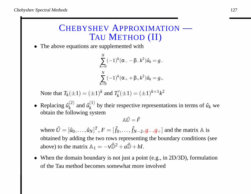
CHEBYSHEV APPROXIMATION —TAU METHOD (II)
• The above equations are supplemented with
N
∑k=0
(−1)k(α−−β−k2)uk = g−
N
∑k=0
(−1)k(α+ +β+k2)uk = g+
Note that Tk(±1) = (±1)k and T ′k (±1) = (±1)k+1k2
• Replacing u(2)k and u(1)
k by their respective representations in terms of uk weobtain the following system
AU = F
where U = [u0, . . . , uN ]T , F = [ f0, . . . , fN−2,g−,g+] and the matrix A is
obtained by adding the two rows representing the boundary conditions (see
above) to the matrix A1 = −νD2 +aD+bI.
• When the domain boundary is not just a point (e.g., in 2D/3D), formulation
of the Tau method becomes somewhat more involved
Chebyshev Spectral Methods 128
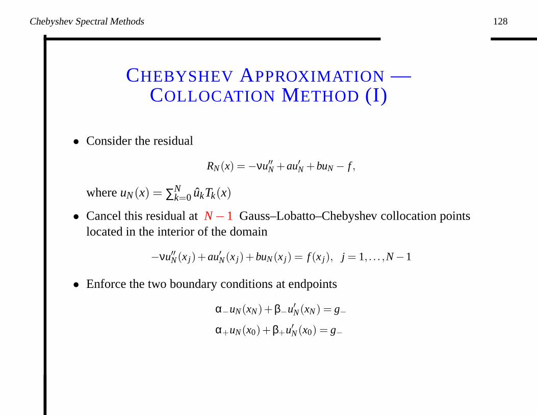
CHEBYSHEV APPROXIMATION —COLLOCATION METHOD (I)
• Consider the residual
RN(x) = −νu′′N +au′N +buN − f ,
where uN(x) = ∑Nk=0 ukTk(x)
• Cancel this residual at N −1 Gauss–Lobatto–Chebyshev collocation pointslocated in the interior of the domain
−νu′′N(x j)+au′N(x j)+buN(x j) = f (x j), j = 1, . . . ,N −1
• Enforce the two boundary conditions at endpoints
α−uN(xN)+β−u′N(xN) = g−
α+uN(x0)+β+u′N(x0) = g−
Chebyshev Spectral Methods 129
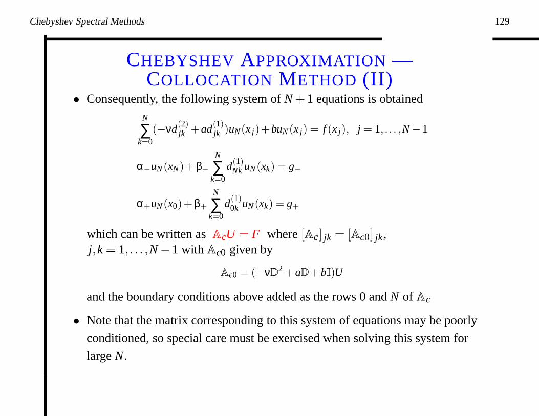
CHEBYSHEV APPROXIMATION —COLLOCATION METHOD (II)
• Consequently, the following system of N +1 equations is obtained
N
∑k=0
(−νd(2)jk +ad(1)
jk )uN(x j)+buN(x j) = f (x j), j = 1, . . . ,N −1
α−uN(xN)+β−
N
∑k=0
d(1)Nk uN(xk) = g−
α+uN(x0)+β+
N
∑k=0
d(1)0k uN(xk) = g+
which can be written as AcU = F where [Ac] jk = [Ac0] jk,j,k = 1, . . . ,N −1 with Ac0 given by
Ac0 = (−νD2 +aD+bI)U
and the boundary conditions above added as the rows 0 and N of Ac
• Note that the matrix corresponding to this system of equations may be poorly
conditioned, so special care must be exercised when solving this system for
large N.
Chebyshev Spectral Methods 130
CHEBYSHEV APPROXIMATION —NONCONSTANT COEFFICIENTS AND NONLINEAR
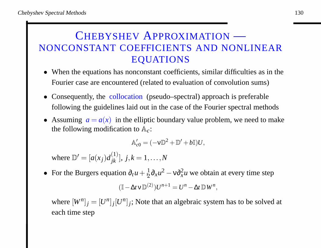
EQUATIONS• When the equations has nonconstant coefficients, similar difficulties as in the
Fourier case are encountered (related to evaluation of convolution sums)
• Consequently, the collocation (pseudo–spectral) approach is preferable
following the guidelines laid out in the case of the Fourier spectral methods
• Assuming a = a(x) in the elliptic boundary value problem, we need to makethe following modification to Ac:
A′c0 = (−νD
2 +D′ +bI)U,
where D′ = [a(x j)d
(1)jk ], j,k = 1, . . . ,N
• For the Burgers equation ∂tu+ 12 ∂xu2 −ν∂2
xu we obtain at every time step
(I−∆t νD(2))Un+1 = Un −∆t DW n,
where [W n] j = [Un] j[Un] j; Note that an algebraic system has to be solved at
each time step
Chebyshev Spectral Methods 131
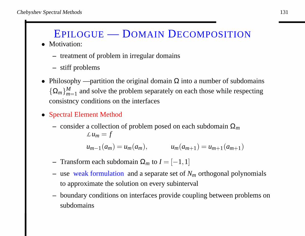
EPILOGUE — DOMAIN DECOMPOSITION• Motivation:
– treatment of problem in irregular domains
– stiff problems
• Philosophy — partition the original domain Ω into a number of subdomains
ΩmMm=1 and solve the problem separately on each those while respecting
consistncy conditions on the interfaces
• Spectral Element Method
– consider a collection of problem posed on each subdomain ΩmLum = f
um−1(am) = um(am), um(am+1) = um+1(am+1)
– Transform each subdomain Ωm to I = [−1,1]
– use weak formulation and a separate set of Nm orthogonal polynomials
to approximate the solution on every subinterval
– boundary conditions on interfaces provide coupling between problems on
subdomains