Ocean Mixed Layer Dynamics and its Impact on Climate Variability

Michael Alexander Earth System Research Lab

http://www.cdc.noaa.gov/people/ michael.alexander/

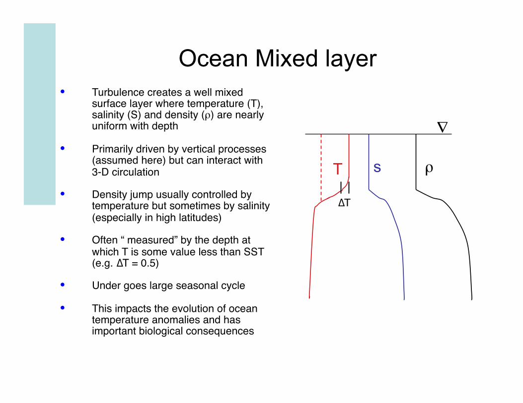
Ocean Mixed layer •  Turbulence creates a well mixed

surface layer where temperature (T), salinity (S) and density (ρ) are nearly uniform with depth

•  Primarily driven by vertical processes (assumed here) but can interact with 3-D circulation

•  Density jump usually controlled by temperature but sometimes by salinity (especially in high latitudes)

•  Often “ measured” by the depth at which T is some value less than SST (e.g. ∆T = 0.5)

•  Under goes large seasonal cycle

•  This impacts the evolution of ocean temperature anomalies and has important biological consequences

∇

T s ρ

∆T

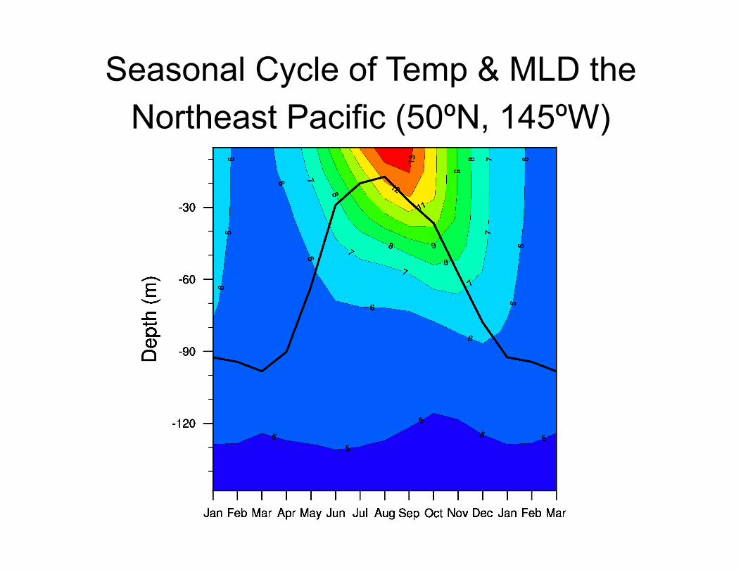
Seasonal Cycle of Temp & MLD the Northeast Pacific (50ºN, 145ºW)

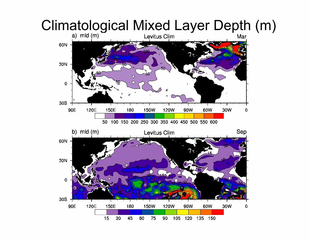
Climatological Mixed Layer Depth (m)

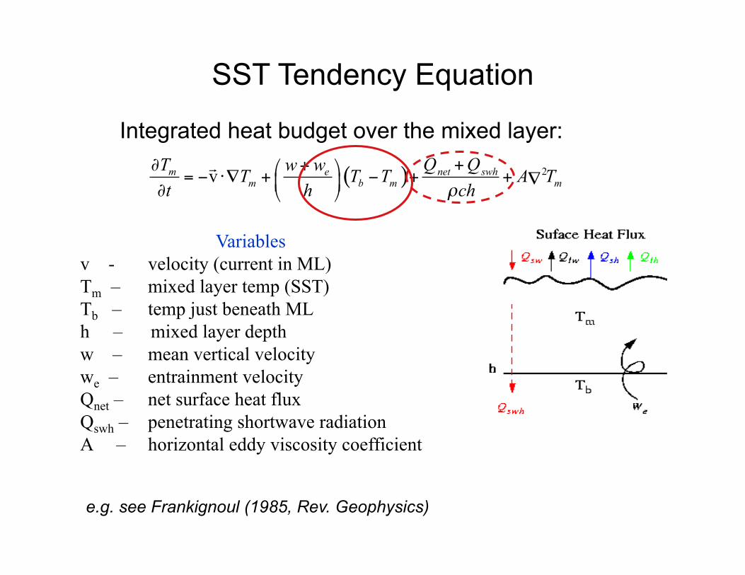
SST Tendency Equation

Variables v - velocity (current in ML) Tm – mixed layer temp (SST) Tb – temp just beneath ML h – mixed layer depth w – mean vertical velocity we – entrainment velocity Qnet – net surface heat flux Qswh – penetrating shortwave radiation A – horizontal eddy viscosity coefficient

( ) 2vm e net swhm b m m

Q QT w wT T T A Tt h chρ

+∂ + = − ⋅∇ + − + + ∇ ∂

e.g. see Frankignoul (1985, Rev. Geophysics)

Integrated heat budget over the mixed layer:

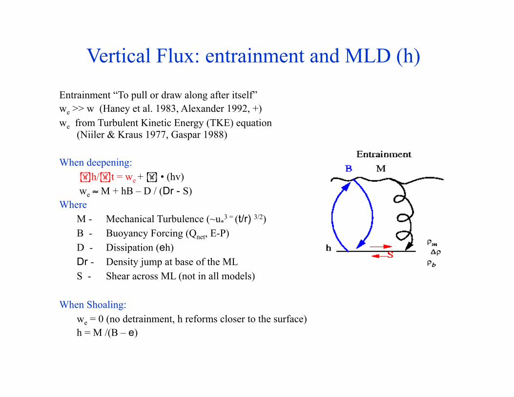
Vertical Flux: entrainment and MLD (h)

Entrainment “To pull or draw along after itself” we >> w (Haney et al. 1983, Alexander 1992, +) we from Turbulent Kinetic Energy (TKE) equation

(Niiler & Kraus 1977, Gaspar 1988)

When deepening: h/t = we + • (hv) we ≈ M + hB – D / (Dr - S) Where M - Mechanical Turbulence (~u*

3 = (t/r) 3/2)

B - Buoyancy Forcing (Qnet, E-P) D - Dissipation (eh) Dr - Density jump at base of the ML S - Shear across ML (not in all models)

When Shoaling: we = 0 (no detrainment, h reforms closer to the surface) h = M /(B – e)

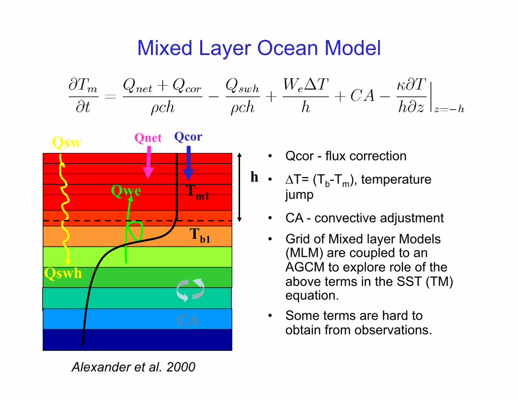
Mixed Layer Ocean Model

h

Tb1

Tm1

Qnet Qcor

Qswh

Qwe

CA

Alexander et al. 2000

Qsw •  Qcor - flux correction

•  ∆T= (Tb-Tm), temperature jump

•  CA - convective adjustment •  Grid of Mixed layer Models

(MLM) are coupled to an AGCM to explore role of the above terms in the SST (TM) equation.

•  Some terms are hard to obtain from observations.

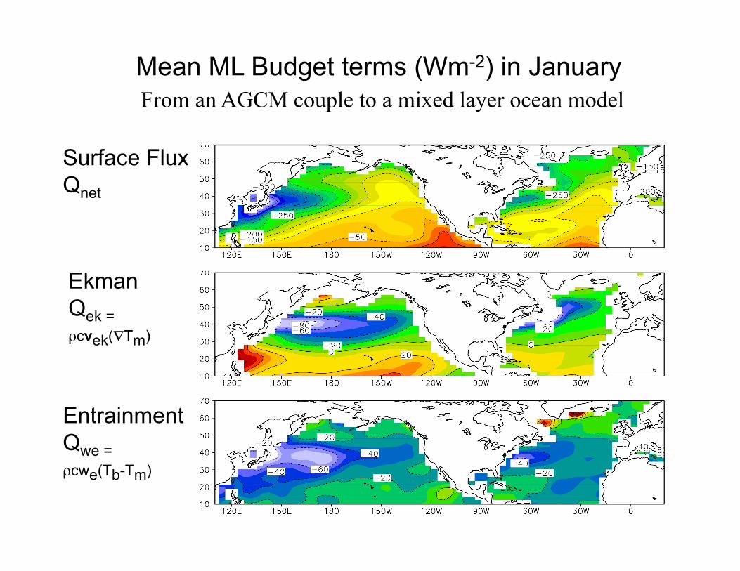
Mean ML Budget terms (Wm-2) in January From an AGCM couple to a mixed layer ocean model

Entrainment Qwe = ρcwe(Tb-Tm)

Ekman Qek = ρcvek(∇Tm)

Surface Flux Qnet

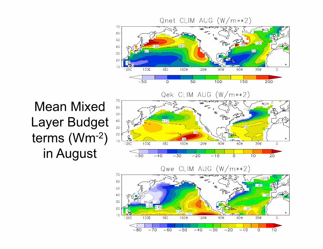
Mean Mixed Layer Budget terms (Wm-2)

in August

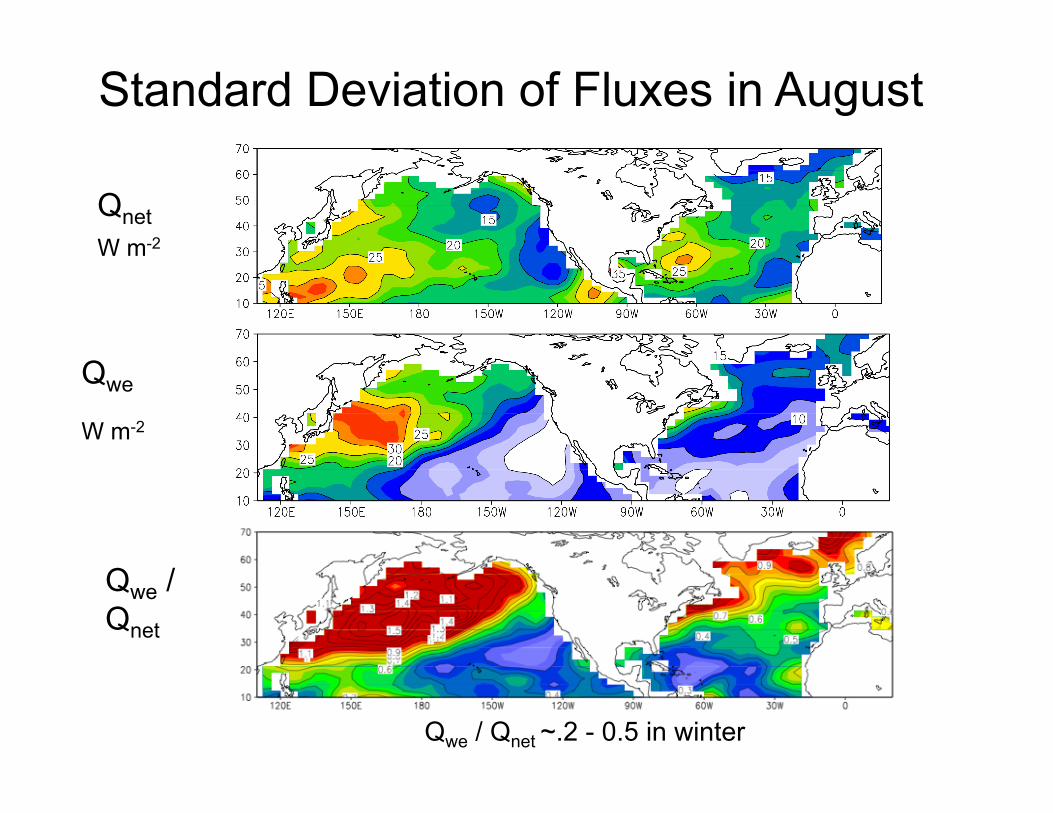
Standard Deviation of Fluxes in August

Qwe

W m-2

Qnet W m-2

Qwe / Qnet

Qwe / Qnet ~.2 - 0.5 in winter

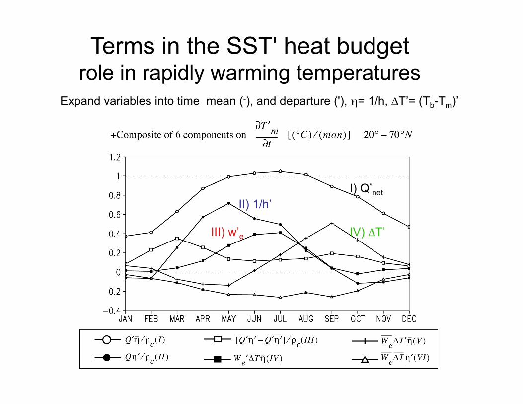
Terms in the SST' heat budget role in rapidly warming temperatures

Expand variables into time mean (-), and departure ('), η= 1/h, ∆T’= (Tb-Tm)’

I) Q’net II) 1/h’

III) w’e IV) ΔT’

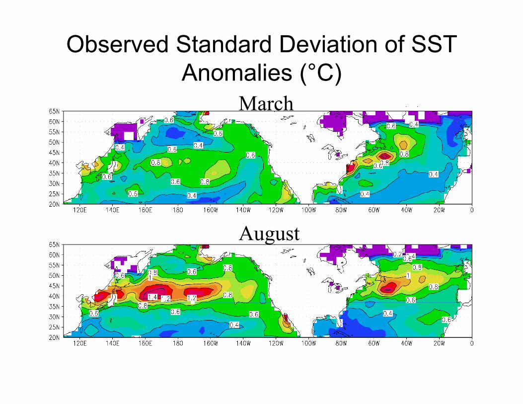
Observed Standard Deviation of SST Anomalies (°C)

August

March

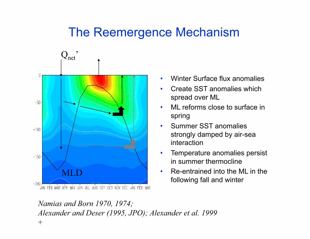
The Reemergence Mechanism

•  Winter Surface flux anomalies •  Create SST anomalies which

spread over ML •  ML reforms close to surface in

spring •  Summer SST anomalies

strongly damped by air-sea interaction

•  Temperature anomalies persist in summer thermocline

•  Re-entrained into the ML in the following fall and winter

Namias and Born 1970, 1974; Alexander and Deser (1995, JPO); Alexander et al. 1999 +

Qnet’

MLD

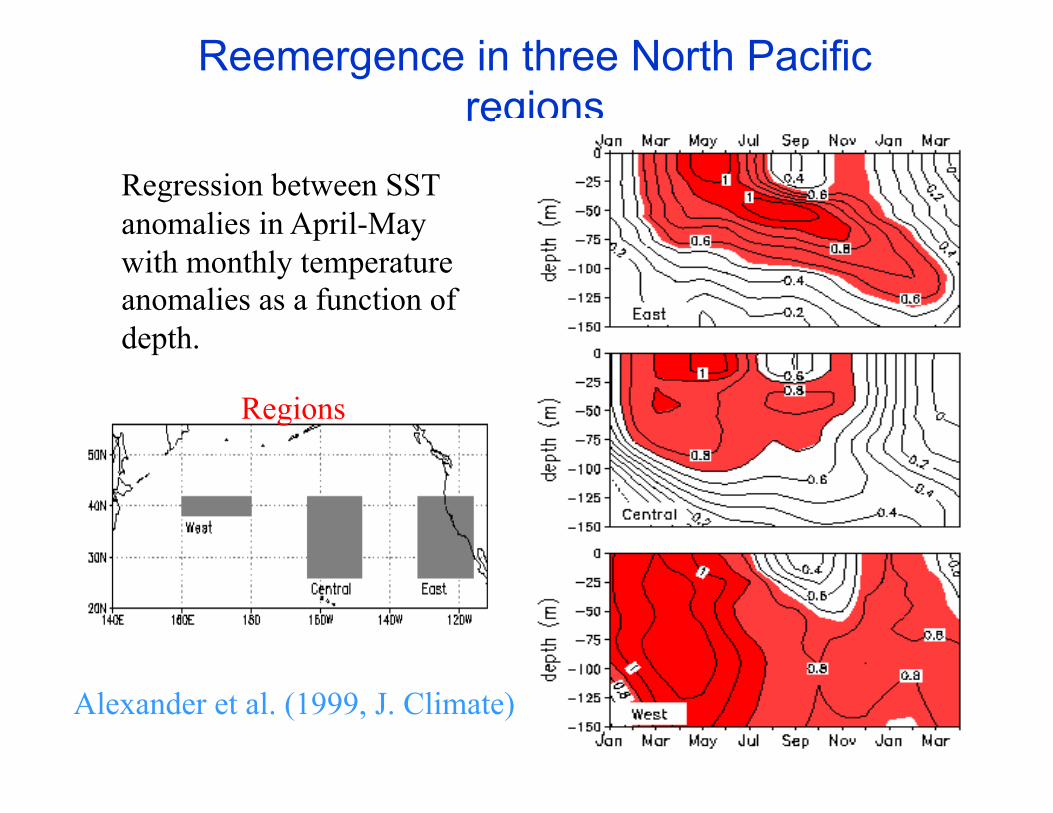
Reemergence in three North Pacific regions

Regression between SST anomalies in April-May with monthly temperature anomalies as a function of depth.

Regions

Alexander et al. (1999, J. Climate)

Reg 2 - Northeast Atlantic (47%)

Timlin, Alexander, Deser, 2002, J.Climate

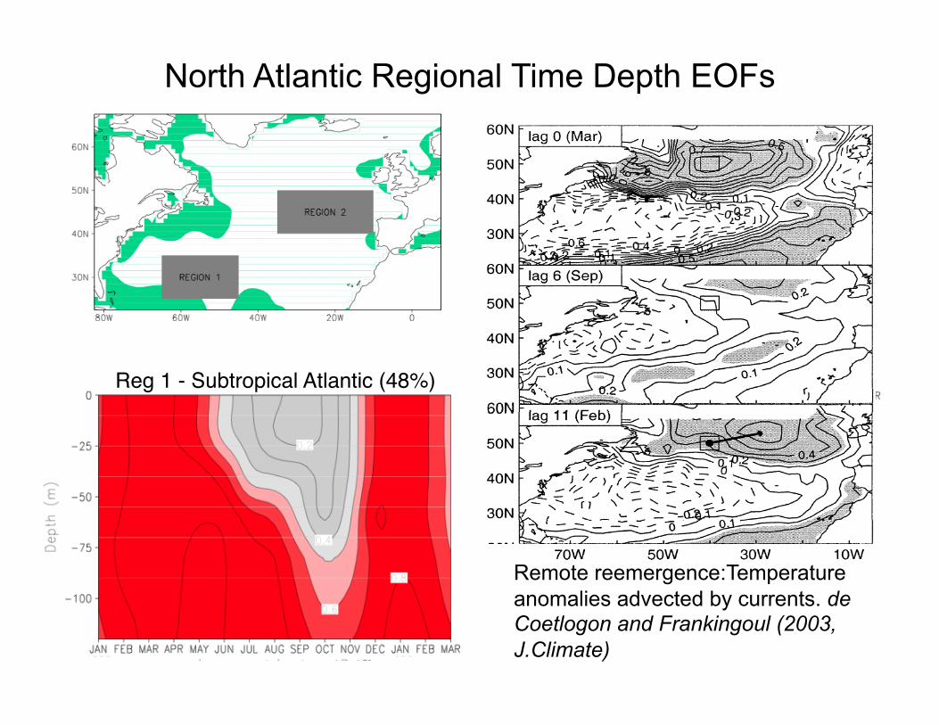
North Atlantic Regional Time Depth EOFs

Reg 1 - Subtropical Atlantic (48%)

Remote reemergence:Temperature anomalies advected by currents. de Coetlogon and Frankingoul (2003, J.Climate)

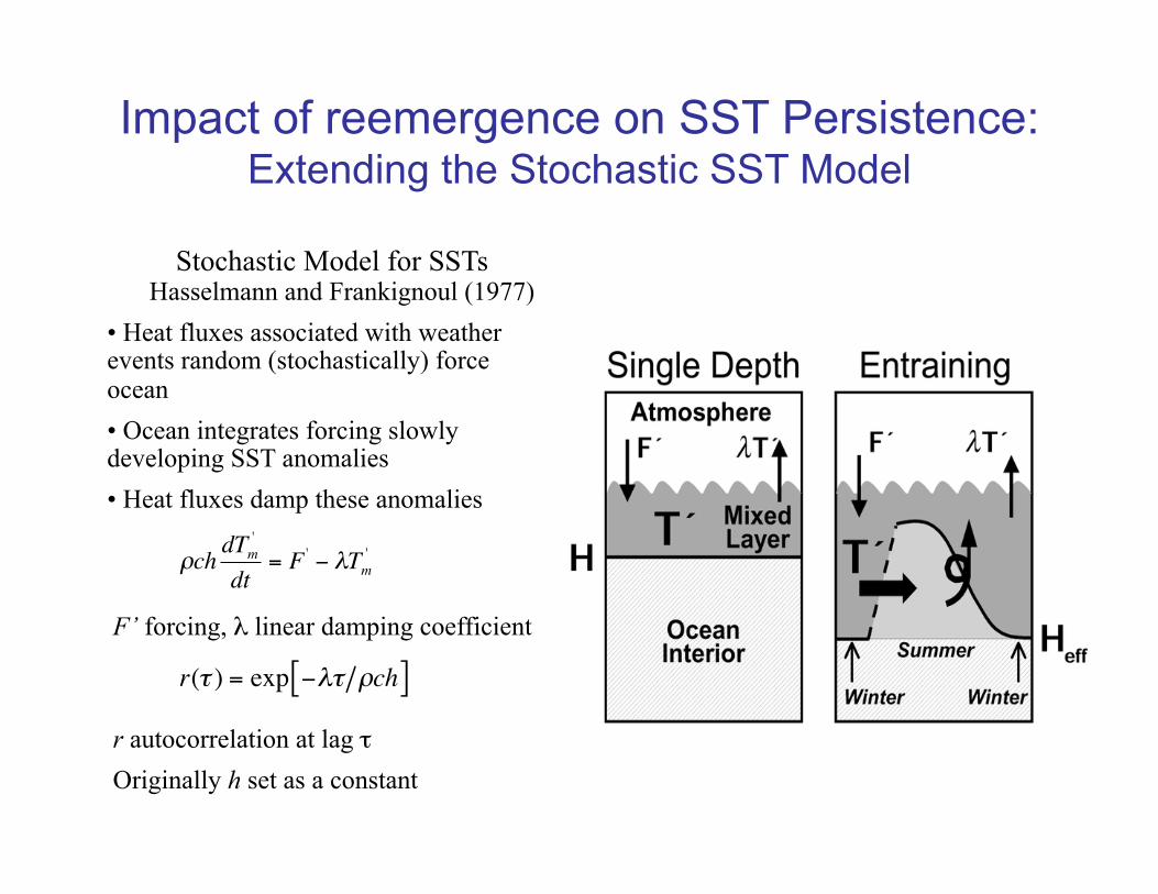
Stochastic Model for SSTs Hasselmann and Frankignoul (1977)

•  Heat fluxes associated with weather events random (stochastically) force ocean •  Ocean integrates forcing slowly developing SST anomalies •  Heat fluxes damp these anomalies

F’ forcing, λ linear damping coefficient

r autocorrelation at lag τ Originally h set as a constant

Impact of reemergence on SST Persistence: Extending the Stochastic SST Model

ρchdTm

'

dt= F ' − λTm

'

r(τ ) = exp −λτ ρch[ ]

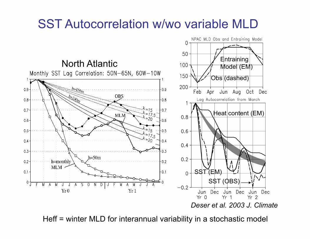
SST Autocorrelation w/wo variable MLD

North Atlantic

Heff = winter MLD for interannual variability in a stochastic model

Deser et al. 2003 J. Climate

Heat content (EM)

Obs (dashed)

Entraining Model (EM)

SST (EM) SST (OBS)

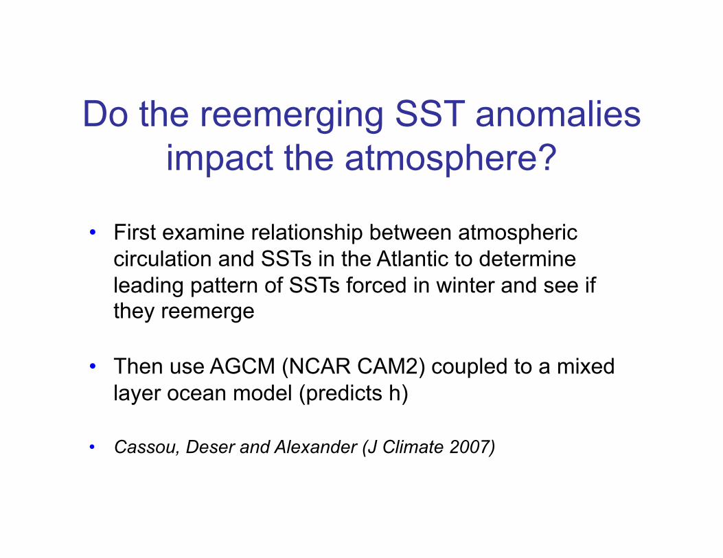
Do the reemerging SST anomalies impact the atmosphere?

•  First examine relationship between atmospheric circulation and SSTs in the Atlantic to determine leading pattern of SSTs forced in winter and see if they reemerge

•  Then use AGCM (NCAR CAM2) coupled to a mixed layer ocean model (predicts h)

•  Cassou, Deser and Alexander (J Climate 2007)

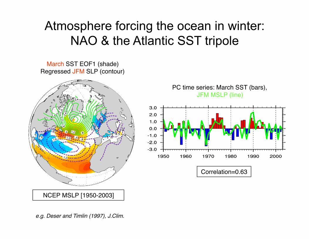
March SST EOF1 (shade) Regressed JFM SLP (contour)

PC time series: March SST (bars), JFM MSLP (line)

NCEP MSLP [1950-2003]

Correlation=0.63

e.g. Deser and Timlin (1997), J.Clim.

Atmosphere forcing the ocean in winter: NAO & the Atlantic SST tripole

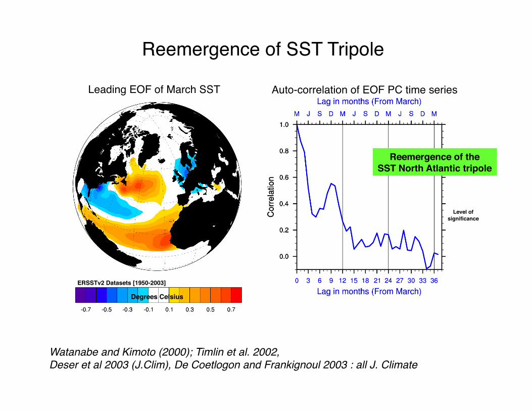
Watanabe and Kimoto (2000); Timlin et al. 2002, Deser et al 2003 (J.Clim), De Coetlogon and Frankignoul 2003 : all J. Climate

Auto-correlation of EOF PC time series

Level of significance

Degrees Celsius

Reemergence of the SST North Atlantic tripole

Leading EOF of March SST

ERSSTv2 Datasets [1950-2003]

Reemergence of SST Tripole

Temperature (Degrees C)

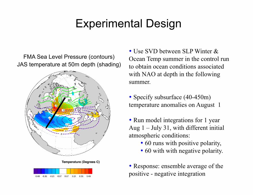
FMA Sea Level Pressure (contours) JAS temperature at 50m depth (shading)

•  Use SVD between SLP Winter & Ocean Temp summer in the control run to obtain ocean conditions associated with NAO at depth in the following summer.

•  Specify subsurface (40-450m) temperature anomalies on August 1

•  Run model integrations for 1 year Aug 1 – July 31, with different initial atmospheric conditions:

•  60 runs with positive polarity, •  60 with with negative polarity.

•  Response: ensemble average of the positive - negative integration

Experimental Design

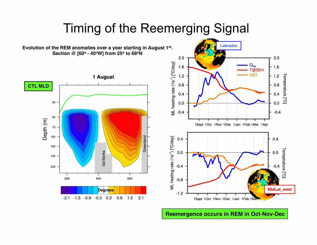
CTL MLD

Labrador

MidLat_west

Reemergence occurs in REM in Oct-Nov-Dec

Degrees

Evolution of the REM anomalies over a year starting in August 1st. Section @ [60o - 40oW] from 25o to 68oN

Timing of the Reemerging Signal

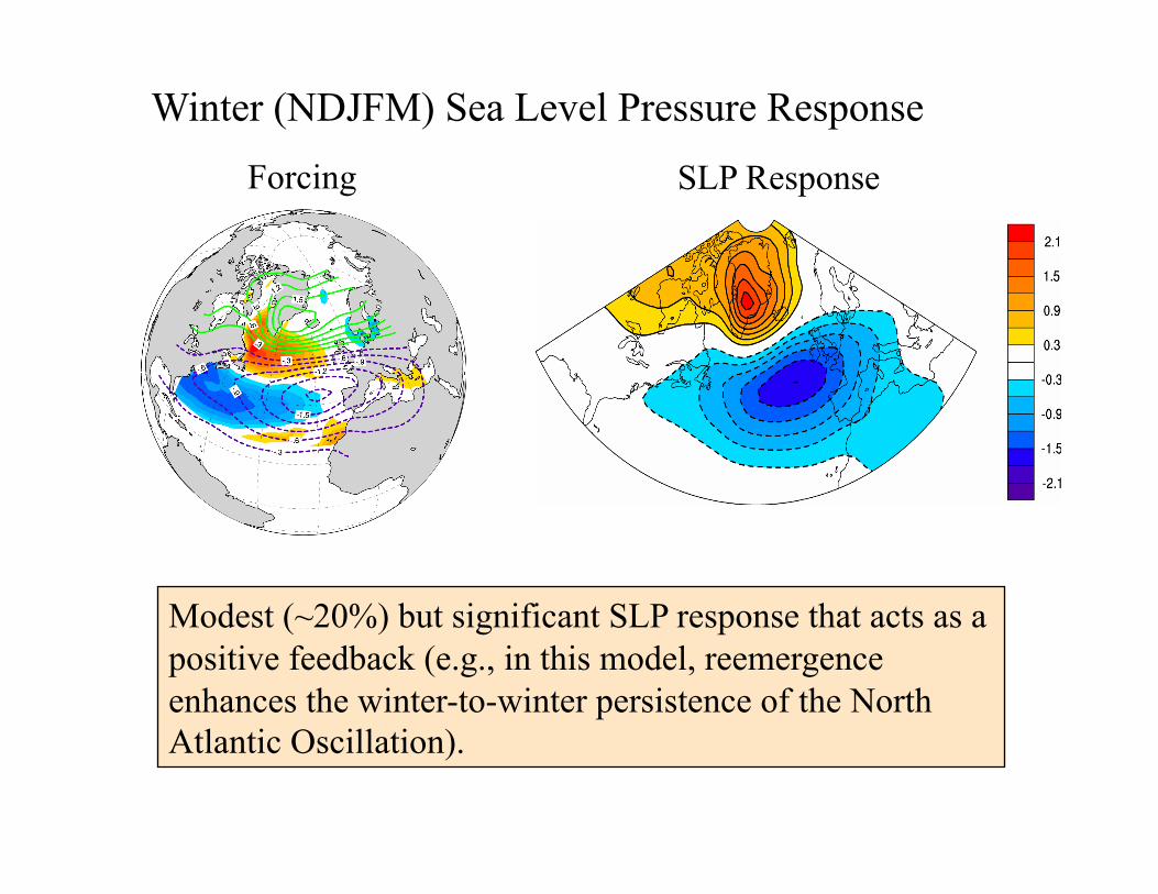
Modest (~20%) but significant SLP response that acts as a positive feedback (e.g., in this model, reemergence enhances the winter-to-winter persistence of the North Atlantic Oscillation).

Forcing

Winter (NDJFM) Sea Level Pressure Response

SLP Response

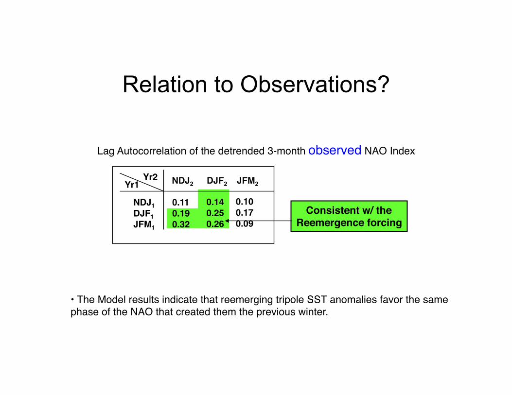
•  The Model results indicate that reemerging tripole SST anomalies favor the same phase of the NAO that created them the previous winter.

Yr1

NDJ1 DJF1 JFM1

NDJ2 DJF2 JFM2

0.11 0.19 0.32

0.14 0.25 0.26

0.10 0.17 0.09

Yr2

Lag Autocorrelation of the detrended 3-month observed NAO Index

Consistent w/ the Reemergence forcing

Relation to Observations?

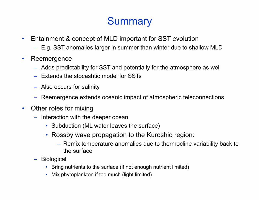
Summary •  Entainment & concept of MLD important for SST evolution

–  E.g. SST anomalies larger in summer than winter due to shallow MLD

•  Reemergence –  Adds predictability for SST and potentially for the atmosphere as well –  Extends the stocashtic model for SSTs

–  Also occurs for salinity

–  Reemergence extends oceanic impact of atmospheric teleconnections

•  Other roles for mixing –  Interaction with the deeper ocean

•  Subduction (ML water leaves the surface) •  Rossby wave propagation to the Kuroshio region:

– Remix temperature anomalies due to thermocline variability back to the surface

–  Biological •  Bring nutrients to the surface (if not enough nutrient limited) •  Mix phytoplankton if too much (light limited)

Additional Slides

• More on the experiment of reemergence in the Atlantic

• Rossby waves that are

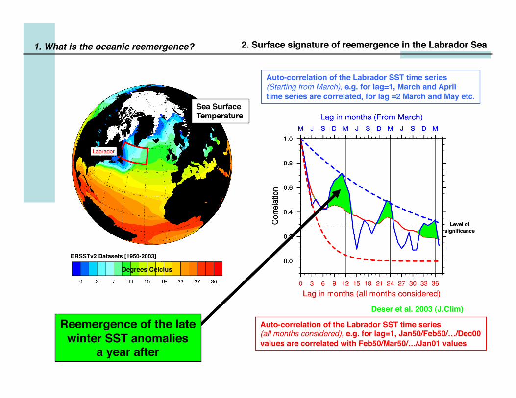
1. What is the oceanic reemergence? 2. Surface signature of reemergence in the Labrador Sea

Sea Surface Temperature

e-folding = ~ 4 mths

Auto-correlation of the Labrador SST time series (all months considered), e.g. for lag=1, Jan50/Feb50/…/Dec00 values are correlated with Feb50/Mar50/…/Jan01 values

e-folding = ~ 36 mths

e-folding = ~ 4 mths

Auto-correlation of the Labrador SST time series (Starting from March), e.g. for lag=1, March and April time series are correlated, for lag =2 March and May etc.

Reemergence of the late winter SST anomalies

a year after

Deser et al. 2003 (J.Clim)

ERSSTv2 Datasets [1950-2003]

Degrees Celcius

Level of significance

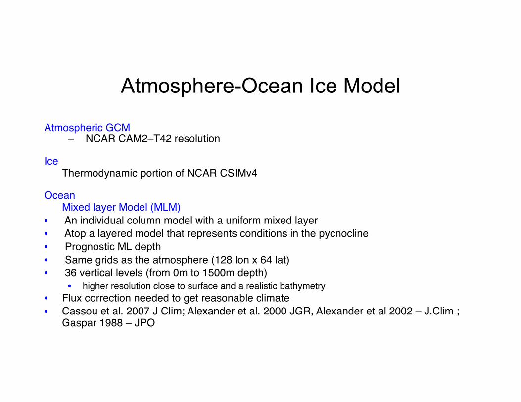
Atmosphere-Ocean Ice Model

Atmospheric GCM –  NCAR CAM2–T42 resolution

Ice Thermodynamic portion of NCAR CSIMv4

Ocean Mixed layer Model (MLM) •  An individual column model with a uniform mixed layer •  Atop a layered model that represents conditions in the pycnocline •  Prognostic ML depth •  Same grids as the atmosphere (128 lon x 64 lat) •  36 vertical levels (from 0m to 1500m depth)

•  higher resolution close to surface and a realistic bathymetry •  Flux correction needed to get reasonable climate •  Cassou et al. 2007 J Clim; Alexander et al. 2000 JGR, Alexander et al 2002 – J.Clim ;

Gaspar 1988 – JPO

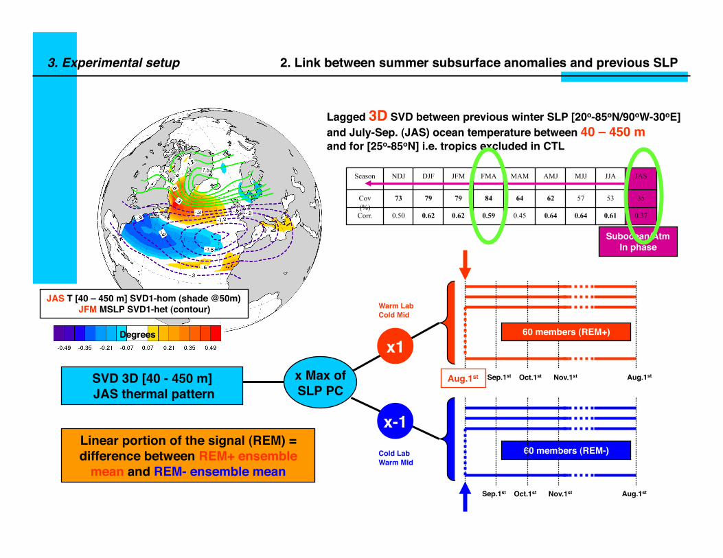
3. Experimental setup 2. Link between summer subsurface anomalies and previous SLP

Lagged 3D SVD between previous winter SLP [20o-85oN/90oW-30oE] and July-Sep. (JAS) ocean temperature between 40 – 450 m and for [25o-85oN] i.e. tropics excluded in CTL

0.37 0.61 0.64 0.64 0.45 0.59 0.62 0.62 0.50 Corr.

35 53 57 62 64 84 79 79 73 Cov (%)

JAS JJA MJJ AMJ MAM FMA JFM DJF NDJ Season

Subocean/Atm In phase

Linear portion of the signal (REM) = difference between REM+ ensemble

mean and REM- ensemble mean

x-1

Sep.1st Oct.1st Aug.1st

60 members (REM-)

Nov.1st

Cold Lab Warm Mid

x1 Aug.1st

60 members (REM+)

Warm Lab Cold Mid

Sep.1st Oct.1st Aug.1st Nov.1st SVD 3D [40 - 450 m] JAS thermal pattern

x Max of SLP PC

Degrees

JAS T [40 – 450 m] SVD1-hom (shade @50m) JFM MSLP SVD1-het (contour)

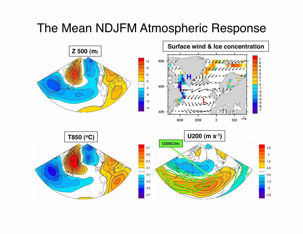
T850 (oC) U200 (m s-1) U200Clim

Z 500 (m) Surface wind & Ice concentration

The Mean NDJFM Atmospheric Response

H

L

Degrees (C°)

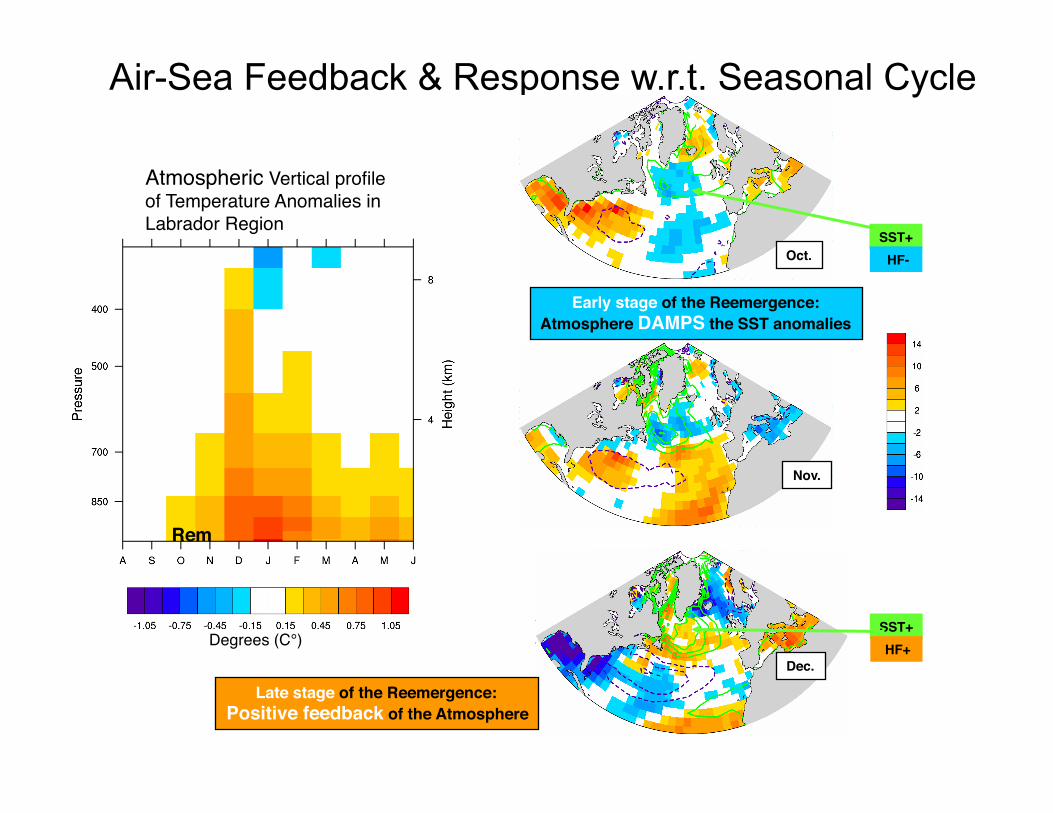
Atmospheric Vertical profile of Temperature Anomalies in Labrador Region

Rem

Air-Sea Feedback & Response w.r.t. Seasonal Cycle

Oct.

Nov.

Early stage of the Reemergence: Atmosphere DAMPS the SST anomalies

SST+ HF-

Color=REM total heat flux (W m-2) Contour =REMSST (oC)

Dec.

Late stage of the Reemergence: Positive feedback of the Atmosphere

SST+ HF+

DEC

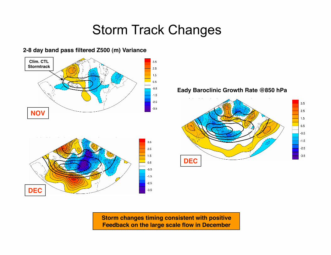
Storm changes timing consistent with positive Feedback on the large scale flow in December

Storm Track Changes

Eady Baroclinic Growth Rate @850 hPa

DEC

2-8 day band pass filtered Z500 (m) Variance

Clim. CTL Stormtrack

NOV

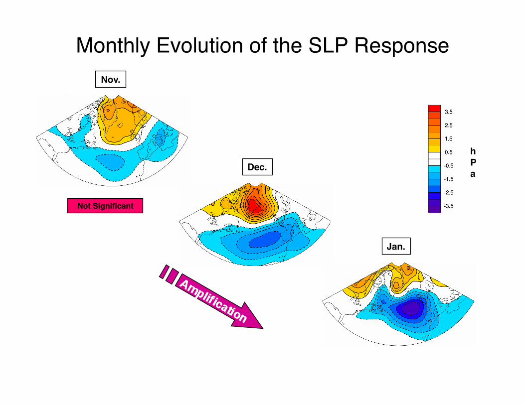
Nov.

Dec.

Jan.

h P a

Not Significant

Monthly Evolution of the SLP Response

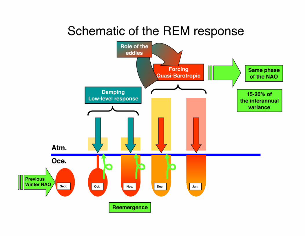
Sept.

Reemergence

Oct. Nov.

Damping Low-level response

Dec. Jan.

Forcing Quasi-Barotropic

Role of the eddies

Previous Winter NAO

Atm.

Oce.

Same phase of the NAO

15-20% of the interannual

variance

Schematic of the REM response

Additional Topics

•  The flux components and their variability •  Schematic of the mixed layer model •  Pattern of atmospheric circulation (SLP) and the

underlying fluxes) •  Basin-wide reemergence •  The Pacific Decadal Oscillation •  Wind generated Rossby waves and its relation to

SSTs •  The Latif and Barnett mechanism for the PDO and

“problems” with this mechanism

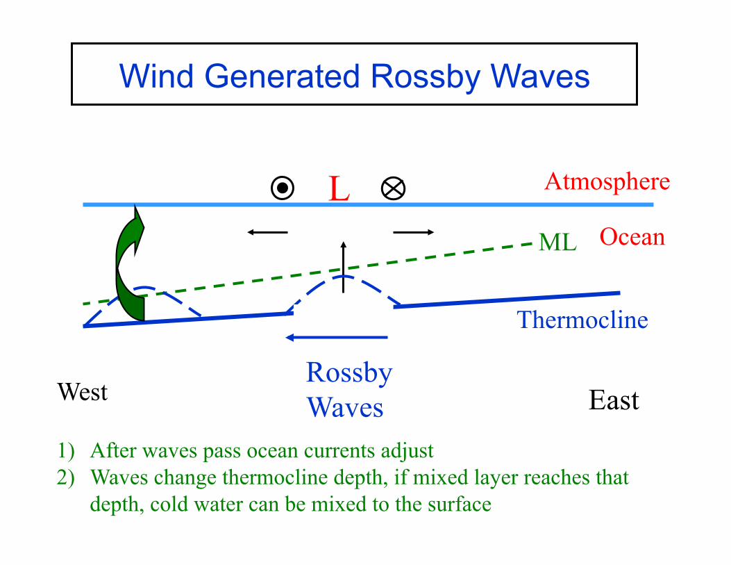
Wind Generated Rossby Waves

West East

Atmosphere

Ocean

Thermocline

ML

L

Rossby Waves

1)  After waves pass ocean currents adjust 2)  Waves change thermocline depth, if mixed layer reaches that

depth, cold water can be mixed to the surface

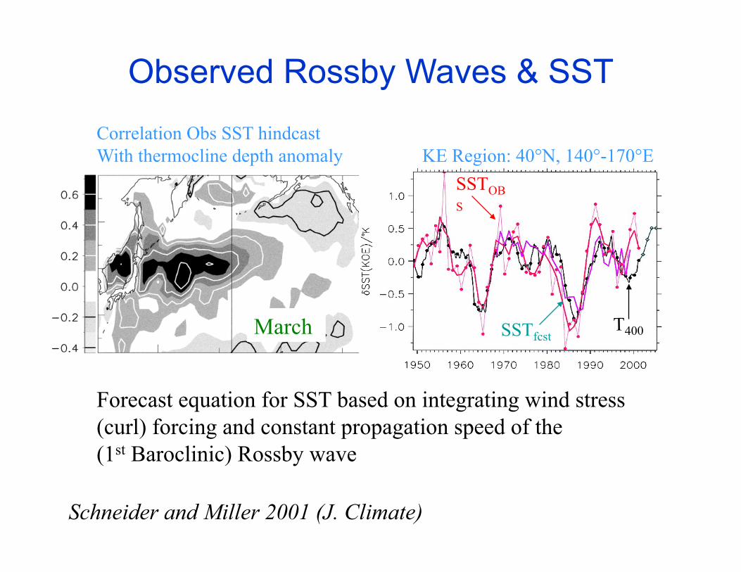
Observed Rossby Waves & SST

t o xP c F τ∂ − ∂ = ∇×∫

Schneider and Miller 2001 (J. Climate)

March

KE Region: 40°N, 140°-170°E SSTOBS

T400 SSTfcst

Correlation Obs SST hindcast With thermocline depth anomaly

Forecast equation for SST based on integrating wind stress (curl) forcing and constant propagation speed of the (1st Baroclinic) Rossby wave

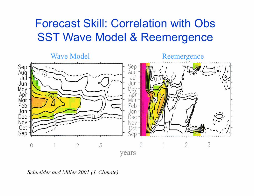
Forecast Skill: Correlation with Obs SST Wave Model & Reemergence

Wave Model Reemergence

years

Schneider and Miller 2001 (J. Climate)

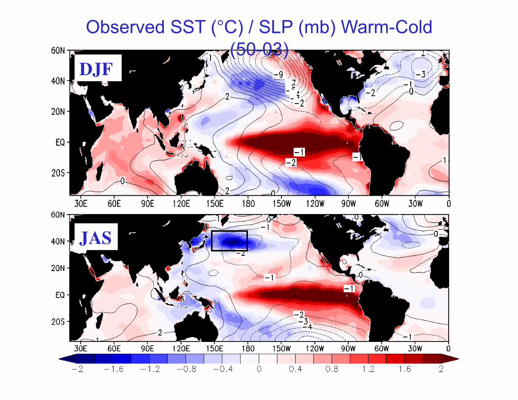
DJF

JAS

Observed SST (°C) / SLP (mb) Warm-Cold (50-03)

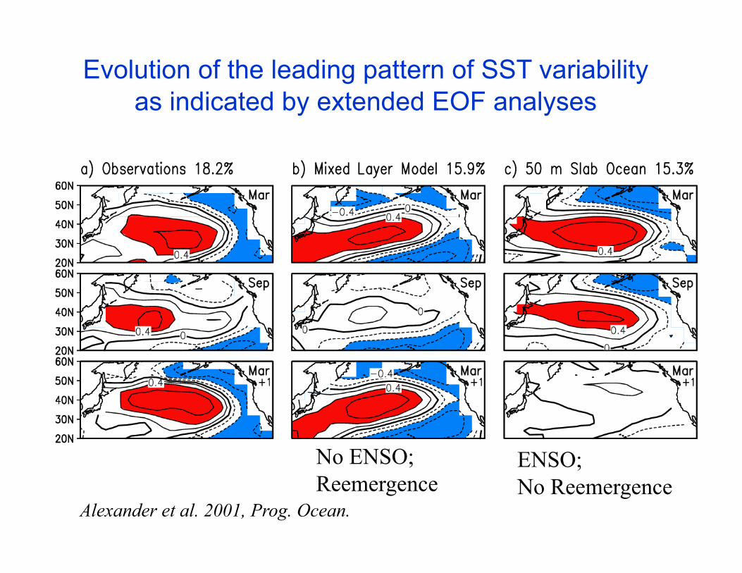
Evolution of the leading pattern of SST variability as indicated by extended EOF analyses

Alexander et al. 2001, Prog. Ocean.

No ENSO; Reemergence

ENSO; No Reemergence

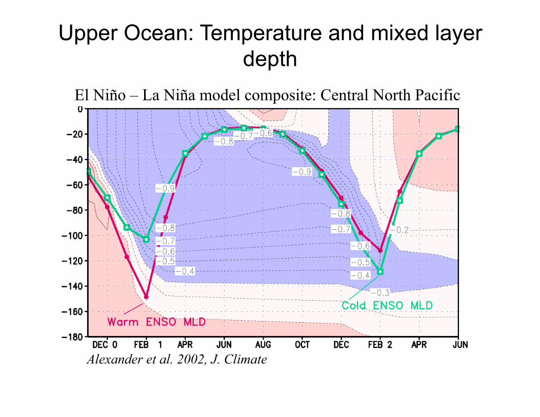
Upper Ocean: Temperature and mixed layer depth

El Niño – La Niña model composite: Central North Pacific

Alexander et al. 2002, J. Climate

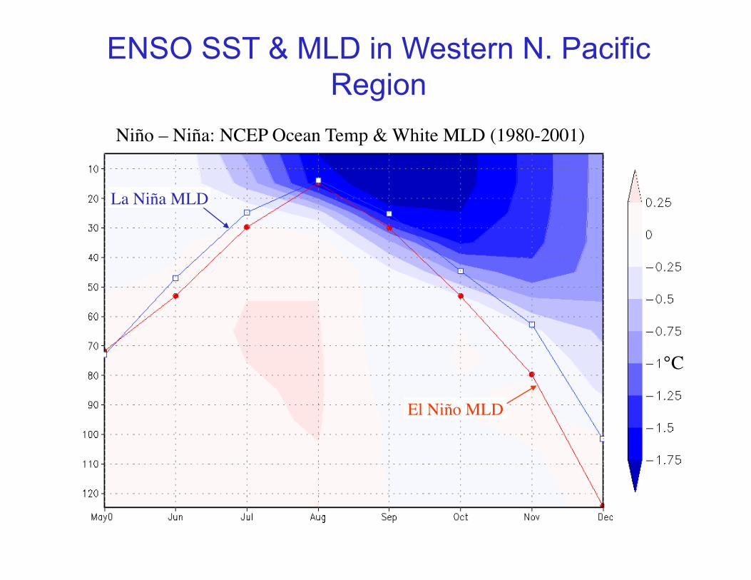
ENSO SST & MLD in Western N. Pacific Region

El Niño MLD

La Niña MLD

Niño – Niña: NCEP Ocean Temp & White MLD (1980-2001)

°C