Observer validation and model based control of a two mass oscillator with backlash

Rafael Fietzek and Stephan Rinderknecht Institute for Mechatronic Systems (IMS)

TU Darmstadt Petersenstr.30, 64287 Darmstadt, Germany

{fietzek & rinderknecht}@ims.tu-darmstadt.de Abstract - In many technical systems, like for example automotive powertrains, the torque generated by the actuator is transmitted through an elastic shaft with backlash, which results in a system where the controlled variable is not collocated with the actuator. A model based pole placement control approach can be used to achieve satisfying closed loop dynamics. However for this approach the system states have to be known, but for cost reasons not every variable can be measured. Therefore a powertrain of an electric car is modeled as a two mass oscillator with backlash and a nonlinear observer is designed to estimate the system states in this paper. The comparison of simulated and measured data is used to validate the performance of the observer depending on the number of measured variables. Index Terms - two mass oscillator, backlash, nonlinear observer, pole placement, electric car powertrain

I. INTRODUCTION

In a powertrain of an electric car, like for example the Tesla roadster, the torque generated by the electric motor is often transmitted through an elastic shaft. For an optimal result regarding the car’s dynamics and the comfort the rotational speed of the wheel should be controlled instead of the rotational speed of the electric motor. However this causes the controlled variable to be non-collocated. Simple PID based controllers have many advantages, but when it comes to the control of non-collocated systems the achievable dynamics are limited and the systems tend to show instable behavior [1]. A model based controller can be used to solve this problem, but for this approach the system state has to be known. Since sensors are expensive, observers are used to estimate the state variables. To get good estimates of the state variables it is essential that nonlinearities are implemented in the observer. The nonlinearities described in section II of this paper are backlash caused by the tripod joint and Coulomb friction generated at the brake disc. These nonlinearities have the biggest impact on the dynamics of the electric powertrain. Furthermore it will be tested how many input variables are necessary to get a good estimate of the wheel hub speed. This observer is based on a Kalman filter with a nonlinear extension to cover the backlash [2],[3],[4]. The main contribution of this paper is addition of a Coulomb friction model and the validation of the observer with measurements in section IV. There are other approaches like for example a sliding mode [5],[6], super twisting observers [7] or a neural network [8], but the presented method can be implemented efficiently and offers good performance. Moreover in section

V of this paper the performance of the observer and the electric powertrain is tested in combination with a pole placement controller and compared to the results achieved with a PI controller. These two controller types are chosen to enable industrial use of the results and to validate the observer. A widespread overview over control of mechanical systems with backlash is given in [9]. With focus on automotive powertrains, [10] summarizes the control approaches. In recent years for example flatness-based [11] and model predictive control [12] approaches were explored by researchers.

II. IDENTIFICATION

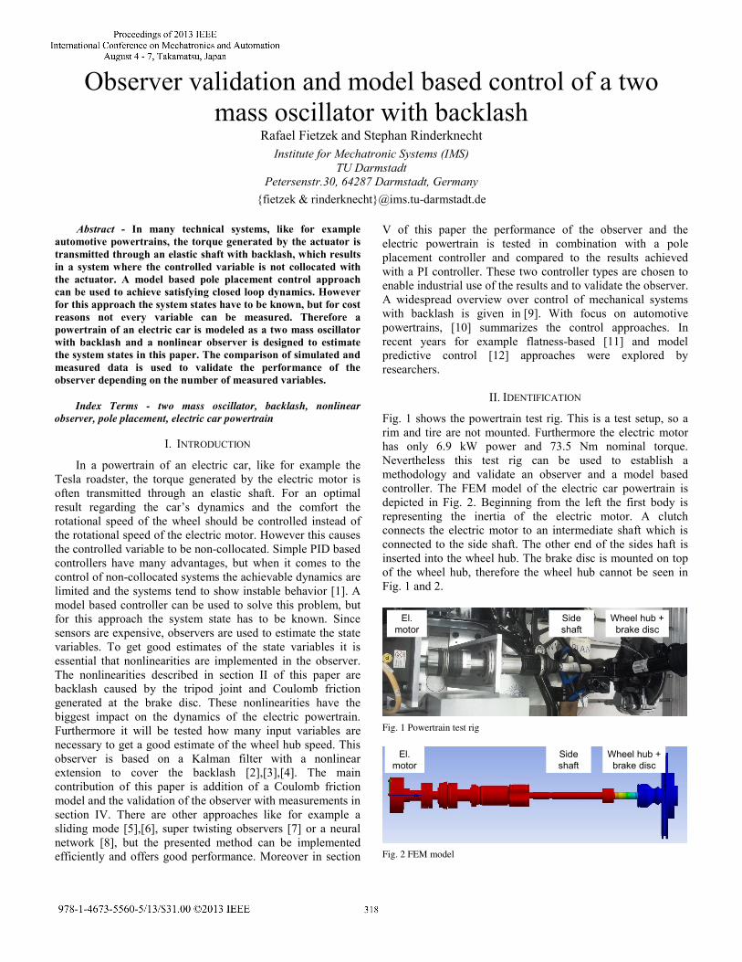
Fig. 1 shows the powertrain test rig. This is a test setup, so a rim and tire are not mounted. Furthermore the electric motor has only 6.9 kW power and 73.5 Nm nominal torque. Nevertheless this test rig can be used to establish a methodology and validate an observer and a model based controller. The FEM model of the electric car powertrain is depicted in Fig. 2. Beginning from the left the first body is representing the inertia of the electric motor. A clutch connects the electric motor to an intermediate shaft which is connected to the side shaft. The other end of the sides haft is inserted into the wheel hub. The brake disc is mounted on top of the wheel hub, therefore the wheel hub cannot be seen in Fig. 1 and 2.

Fig. 1 Powertrain test rig

Fig. 2 FEM model

Side shaft

El. motor

Wheel hub + brake disc

Side shaft

El. motor

Wheel hub + brake disc

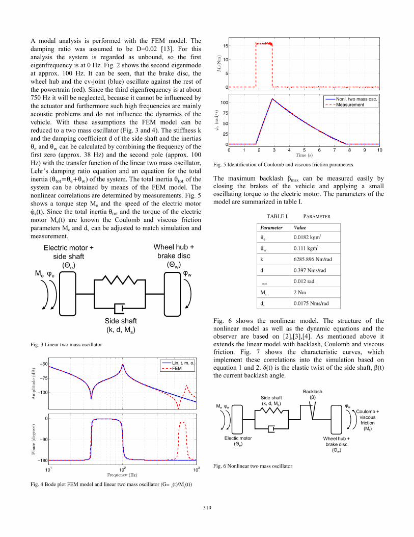
A modal analysis is performed with the FEM model. The damping ratio was assumed to be D=0.02 [13]. For this analysis the system is regarded as unbound, so the first eigenfrequency is at 0 Hz. Fig. 2 shows the second eigenmode at approx. 100 Hz. It can be seen, that the brake disc, the wheel hub and the cv-joint (blue) oscillate against the rest of the powertrain (red). Since the third eigenfrequency is at about 750 Hz it will be neglected, because it cannot be influenced by the actuator and furthermore such high frequencies are mainly acoustic problems and do not influence the dynamics of the vehicle. With these assumptions the FEM model can be reduced to a two mass oscillator (Fig. 3 and 4). The stiffness k and the damping coefficient d of the side shaft and the inertias θe and θw can be calculated by combining the frequency of the first zero (approx. 38 Hz) and the second pole (approx. 100 Hz) with the transfer function of the linear two mass oscillator, Lehr’s damping ratio equation and an equation for the total inertia (θtot θe θw) of the system. The total inertia θtot of the system can be obtained by means of the FEM model. The nonlinear correlations are determined by measurements. Fig. 5 shows a torque step Me and the speed of the electric motor φe(t). Since the total inertia θtot and the torque of the electric motor Me(t) are known the Coulomb and viscous friction parameters Mc and dv can be adjusted to match simulation and measurement.

Fig. 3 Linear two mass oscillator

Fig. 4 Bode plot FEM model and linear two mass oscillator (G= e(t)/Me(t))

Fig. 5 Identification of Coulomb and viscous friction parameters

The maximum backlash βmax can be measured easily by closing the brakes of the vehicle and applying a small oscillating torque to the electric motor. The parameters of the model are summarized in table I.

TABLE I. PARAMETER

Parameter Value θe 0.0182 kgm2 θw 0.111 kgm2

k 6285.896 Nm/rad

d 0.397 Nms/rad

max 0.012 rad

Mc 2 Nm

dv 0.0175 Nms/rad

Fig. 6 shows the nonlinear model. The structure of the nonlinear model as well as the dynamic equations and the observer are based on [2],[3],[4]. As mentioned above it extends the linear model with backlash, Coulomb and viscous friction. Fig. 7 shows the characteristic curves, which implement these correlations into the simulation based on equation 1 and 2. δ(t) is the elastic twist of the side shaft, β(t) the current backlash angle.

Fig. 6 Nonlinear two mass oscillator

Electric motor + side shaft

(Θe)

Wheel hub +brake disc

(Θw)

Side shaft(k, d, Ms)

φeMe φw

−100

−75

−50

Amplitude(dB)

Lin. t. m. o.FEM

101

102

103

−180

−90

0

Frequency (Hz)

Phase

(degrees)

0

5

10

15

Me(N

m)

0 1 2 3 4 5 6 7 8 9 100

25

50

75

100

Time (s)

ϕ̇e(rad/s)

Nonl. two mass osc.Measurement

Electic motor(Θe)

Wheel hub +brake disc

(Θw)

φe φw

Side shaft(k, d, Ms)

Backlash(β)

MeCoulomb +

viscousfriction

(Mf)

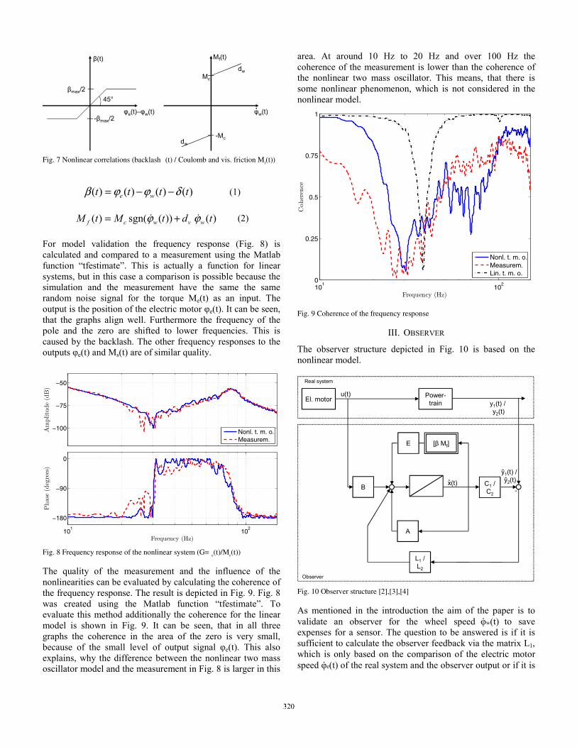
Fig. 7 Nonlinear correlations (backlash (t) / Coulomb and vis. friction Mf(t))

)()()()( tttt we δϕϕβ −−= (1)

)())(sgn()( tdtMtM wvwcf ϕϕ += (2)

For model validation the frequency response (Fig. 8) is calculated and compared to a measurement using the Matlab function “tfestimate”. This is actually a function for linear systems, but in this case a comparison is possible because the simulation and the measurement have the same the same random noise signal for the torque Me(t) as an input. The output is the position of the electric motor φe(t). It can be seen, that the graphs align well. Furthermore the frequency of the pole and the zero are shifted to lower frequencies. This is caused by the backlash. The other frequency responses to the outputs φe(t) and Ms(t) are of similar quality.

Fig. 8 Frequency response of the nonlinear system (G= e(t)/Me(t))

The quality of the measurement and the influence of the nonlinearities can be evaluated by calculating the coherence of the frequency response. The result is depicted in Fig. 9. Fig. 8 was created using the Matlab function “tfestimate”. To evaluate this method additionally the coherence for the linear model is shown in Fig. 9. It can be seen, that in all three graphs the coherence in the area of the zero is very small, because of the small level of output signal φe(t). This also explains, why the difference between the nonlinear two mass oscillator model and the measurement in Fig. 8 is larger in this

area. At around 10 Hz to 20 Hz and over 100 Hz the coherence of the measurement is lower than the coherence of the nonlinear two mass oscillator. This means, that there is some nonlinear phenomenon, which is not considered in the nonlinear model.

Fig. 9 Coherence of the frequency response

III. OBSERVER

The observer structure depicted in Fig. 10 is based on the nonlinear model.

Fig. 10 Observer structure [2],[3],[4]

As mentioned in the introduction the aim of the paper is to validate an observer for the wheel speed φw(t) to save expenses for a sensor. The question to be answered is if it is sufficient to calculate the observer feedback via the matrix L1, which is only based on the comparison of the electric motor speed φe(t) of the real system and the observer output or if it is

βmax/2

-βmax/2φe(t)–φw(t)

β(t)

45°

Mc

φw(t)

Mf(t)

-Mc

dw

dw

−100

−75

−50

Amplitude(dB)

Nonl. t. m. o.Measurem.

101

102

−180

−90

0

Frequency (Hz)

Phase

(degrees)

101

102

0

0.25

0.5

0.75

1

Frequency (Hz)Coheren

ce

Nonl. t. m. o.Measurem.Lin. t. m. o.

u(t) Power-train

B

E

A

x(t) C1 / C2

[β Mf]

-

L1 / L2

Real system

Observer

ŷ1(t) /ŷ2(t)

y1(t) /y2(t)

El. motor

ˆ

necessary to add the side shaft torque Ms(t). Therefore both observers are based on the same linear model, with the nonlinear expansion shown in equation 3, but have different output matrices C1 (4) and C2 (5) and different feedback matrices L1 and L2. To calculate the torque Ms(t) the backlash β(t) has to be subtracted from the first state φe(t)-φw(t). This is not shown in Fig. 10 and Fig. 11 for clearness reasons.

odelmLinear

tu

e

B

e

tx

w

e

we

A

www

eee

tx

w

e

we

tMtt

tt

ddkddk

tt

tt

)(

)(ˆ)(ˆ

)(0

10

)()(

)()(110

)()(

)()(

⎥⎥⎥

⎦

⎤

⎢⎢⎢

⎣

⎡Θ+

⎥⎥⎥

⎦

⎤

⎢⎢⎢

⎣

⎡ −

⎥⎥⎥

⎦

⎤

⎢⎢⎢

⎣

⎡

Θ−ΘΘΘΘ−Θ−

−=

⎥⎥⎥

⎦

⎤

⎢⎢⎢

⎣

⎡ −

ϕϕ

ϕϕ

ϕϕ

ϕϕ

pansionexNonlinear

f

E

ww

e tMt

kk ⎥

⎦

⎤⎢⎣

⎡

⎥⎥⎥

⎦

⎤

⎢⎢⎢

⎣

⎡

ΘΘ−Θ+

)()(

1000

β (3)

⎟⎟⎟⎟⎟⎟

⎠

⎞

⎜⎜⎜⎜⎜⎜

⎝

⎛

⎥⎥⎥

⎦

⎤

⎢⎢⎢

⎣

⎡−

⎥⎥⎥

⎦

⎤

⎢⎢⎢

⎣

⎡ −

⎥⎦

⎤⎢⎣

⎡ −=⎥

⎦

⎤⎢⎣

⎡

00

)(

)()(

)()(

010)()(

)(ˆ)(ˆ 22

t

tt

ttddk

ttM

tx

w

e

we

Cty

e

s

β

ϕϕ

ϕϕ

ϕ

(4)

[ ]

)(ˆ

)(ˆ )()(

)()(010)(

11

tx

w

e

we

Ctye

tt

ttt

⎥⎥⎥

⎦

⎤

⎢⎢⎢

⎣

⎡ −=

ϕϕ

ϕϕϕ

(5)

It should be mentioned that the linear system has full observability for the C1 and C2 matrix, so the basic requirements are fulfilled to obtain all the system states with the observer. The difference between the real system and the observer is feedbacked through the matrices L1 or L2 respectively. These matrices are computed by solving the Riccati equation (6), so the observer has the same structure as a Kalman filter [14]. This method is of course only applicable to the linear systems, therefore the nonlinearities have to be neglected.

12/12/12/12/1

2/12/12/12/12/12/12/12/1 0−=

=+−+

RCPL

QPCRCPAPAPT

TT

(6)

To calculate the solutions P1, P2 to the Riccati equation (6) the matrices R1, R2 and Q1, Q2 (7) have to be calculated.

)()()()()()()(

2/12/1 ttxCtyttButAxtx

νε

+=++=

(7)

Basically R1, R2 can be defined by calculating the covariance matrix of the process noise ε(t) and Q1, Q2 by calculating the covariance matrix of the observation noise ν(t), but for a first

simulative analysis R1, R2 and Q1, Q2 can also be estimated by an educated guess [14]. Since the observer then already performs well regarding the measurements, the effort of calculating the covariance matrices will be waived. Both matrices are set according to [14] as diagonal matrices. The entries of Q1 and Q2 were set iteratively. It turned out, that the entry corresponding to the first state φe(t)-φw(t) had the biggest impact on the observer output, and therefore the value is set lower compared to the other two states. The first entry of the R2 matrix corresponding to the torque measurement is set to a higher value than the second entry, since the torque sensor produces a higher noise level than the encoder.

⎥⎦

⎤⎢⎣

⎡==

⎥⎥⎥

⎦

⎤

⎢⎢⎢

⎣

⎡=

10010

1100000

010000001

212/1 RRQ (8)

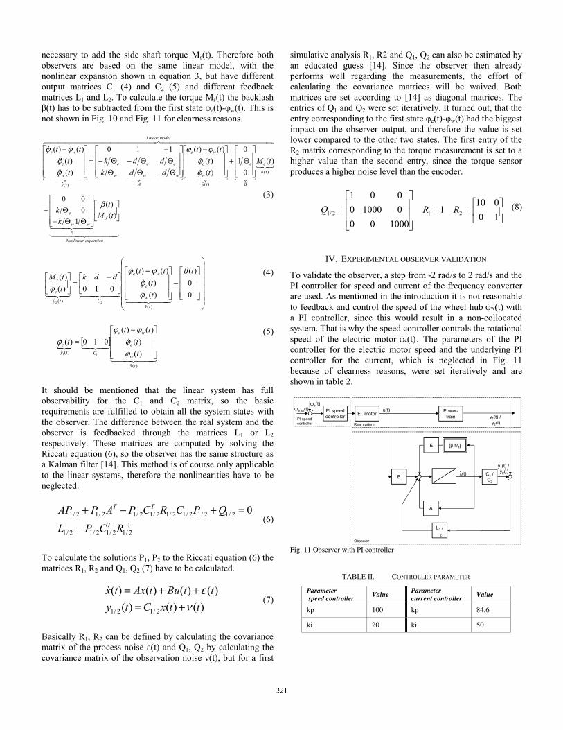
IV. EXPERIMENTAL OBSERVER VALIDATION

To validate the observer, a step from -2 rad/s to 2 rad/s and the PI controller for speed and current of the frequency converter are used. As mentioned in the introduction it is not reasonable to feedback and control the speed of the wheel hub φw(t) with a PI controller, since this would result in a non-collocated system. That is why the speed controller controls the rotational speed of the electric motor φe(t). The parameters of the PI controller for the electric motor speed and the underlying PI controller for the current, which is neglected in Fig. 11 because of clearness reasons, were set iteratively and are shown in table 2.

Fig. 11 Observer with PI controller

TABLE II. CONTROLLER PARAMETER

Parameter speed controller Value

Parameter current controller Value

kp 100 kp 84.6

ki 20 ki 50

u(t) Power-train

B

E

A

x(t) C1 / C2

[β Mf]

-

L1 / L2

Real system

Observer

ŷ1(t) /ŷ2(t)

y1(t) /y2(t)

El. motor

ˆ

-ωe sp(t) PI speedcontroller

ωe(t)

PI speedcontroller

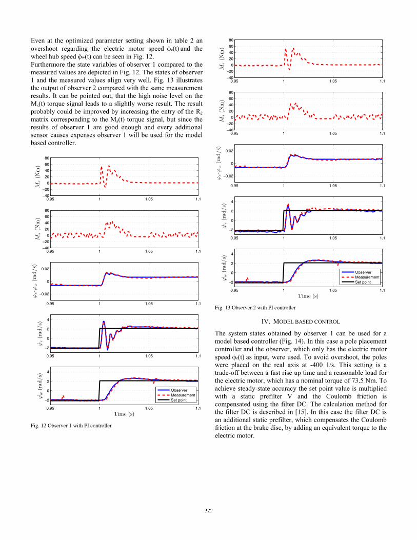
Even at the optimized parameter setting shown in table 2 an overshoot regarding the electric motor speed φe(t) and the wheel hub speed φw(t) can be seen in Fig. 12. Furthermore the state variables of observer 1 compared to the measured values are depicted in Fig. 12. The states of observer 1 and the measured values align very well. Fig. 13 illustrates the output of observer 2 compared with the same measurement results. It can be pointed out, that the high noise level on the Ms(t) torque signal leads to a slightly worse result. The result probably could be improved by increasing the entry of the R2 matrix corresponding to the Ms(t) torque signal, but since the results of observer 1 are good enough and every additional sensor causes expenses observer 1 will be used for the model based controller.

Fig. 12 Observer 1 with PI controller

Fig. 13 Observer 2 with PI controller

IV. MODEL BASED CONTROL

The system states obtained by observer 1 can be used for a model based controller (Fig. 14). In this case a pole placement controller and the observer, which only has the electric motor speed φe(t) as input, were used. To avoid overshoot, the poles were placed on the real axis at -400 1/s. This setting is a trade-off between a fast rise up time and a reasonable load for the electric motor, which has a nominal torque of 73.5 Nm. To achieve steady-state accuracy the set point value is multiplied with a static prefilter V and the Coulomb friction is compensated using the filter DC. The calculation method for the filter DC is described in [15]. In this case the filter DC is an additional static prefilter, which compensates the Coulomb friction at the brake disc, by adding an equivalent torque to the electric motor.

0.95 1 1.05 1.1−40

−20

0

20

40

60

80

Me(N

m)

0.95 1 1.05 1.1−40

−20

0

20

40

60

80

Ms(N

m)

0.95 1 1.05 1.1

−0.02

0

0.02

ϕe-ϕ

w(rad/s)

0.95 1 1.05 1.1

−2

0

2

4

ϕ̇e(rad/s)

0.95 1 1.05 1.1

−2

0

2

4

Time (s)

ϕ̇w(rad/s)

ObserverMeasurementSet point

0.95 1 1.05 1.1−40

−20

0

20

40

60

80

Me(N

m)

0.95 1 1.05 1.1−40

−20

0

20

40

60

80

Ms(N

m)

0.95 1 1.05 1.1

−0.02

0

0.02

ϕe-ϕ

w(rad/s)

0.95 1 1.05 1.1

−2

0

2

4

ϕ̇e(rad/s)

0.95 1 1.05 1.1

−2

0

2

4

Time (s)

ϕ̇w(rad/s)

ObserverMeasurementSet point

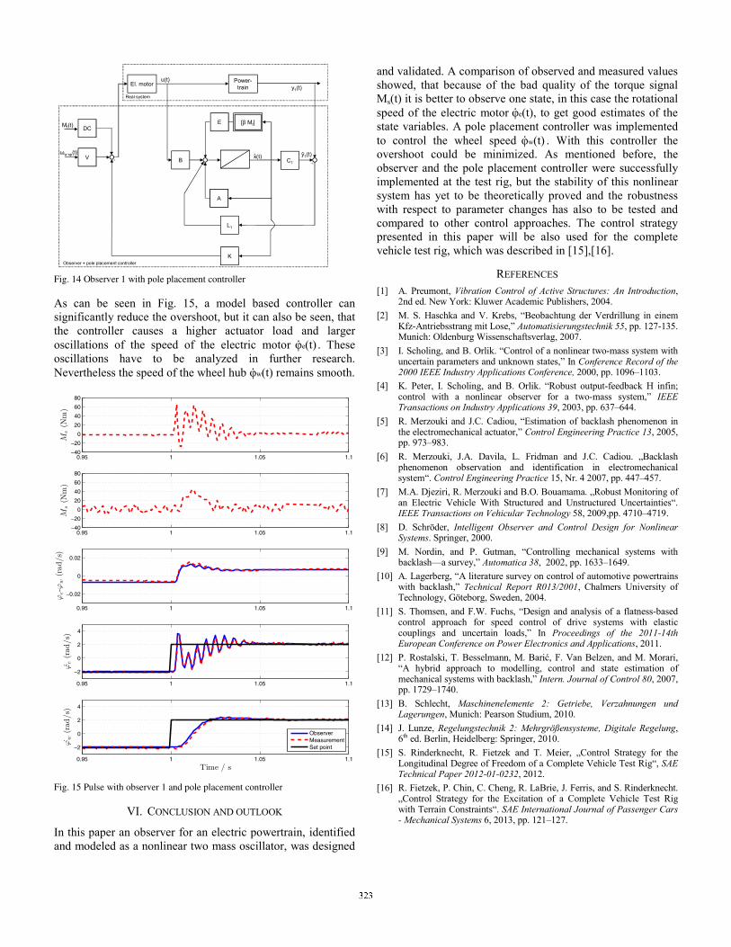
Fig. 14 Observer 1 with pole placement controller

As can be seen in Fig. 15, a model based controller can significantly reduce the overshoot, but it can also be seen, that the controller causes a higher actuator load and larger oscillations of the speed of the electric motor φe(t) . These oscillations have to be analyzed in further research. Nevertheless the speed of the wheel hub φw(t) remains smooth.

Fig. 15 Pulse with observer 1 and pole placement controller

VI. CONCLUSION AND OUTLOOK

In this paper an observer for an electric powertrain, identified and modeled as a nonlinear two mass oscillator, was designed

and validated. A comparison of observed and measured values showed, that because of the bad quality of the torque signal Ms(t) it is better to observe one state, in this case the rotational speed of the electric motor φe(t), to get good estimates of the state variables. A pole placement controller was implemented to control the wheel speed φw(t) . With this controller the overshoot could be minimized. As mentioned before, the observer and the pole placement controller were successfully implemented at the test rig, but the stability of this nonlinear system has yet to be theoretically proved and the robustness with respect to parameter changes has also to be tested and compared to other control approaches. The control strategy presented in this paper will be also used for the complete vehicle test rig, which was described in [15],[16].

REFERENCES [1] A. Preumont, Vibration Control of Active Structures: An Introduction,

2nd ed. New York: Kluwer Academic Publishers, 2004. [2] M. S. Haschka and V. Krebs, “Beobachtung der Verdrillung in einem

Kfz-Antriebsstrang mit Lose,” Automatisierungstechnik 55, pp. 127-135. Munich: Oldenburg Wissenschaftsverlag, 2007.

[3] I. Scholing, and B. Orlik. “Control of a nonlinear two-mass system with uncertain parameters and unknown states,” In Conference Record of the 2000 IEEE Industry Applications Conference, 2000, pp. 1096–1103.

[4] K. Peter, I. Scholing, and B. Orlik. “Robust output-feedback H infin; control with a nonlinear observer for a two-mass system,” IEEE Transactions on Industry Applications 39, 2003, pp. 637–644.

[5] R. Merzouki and J.C. Cadiou, “Estimation of backlash phenomenon in the electromechanical actuator,” Control Engineering Practice 13, 2005, pp. 973–983.

[6] R. Merzouki, J.A. Davila, L. Fridman and J.C. Cadiou. „Backlash phenomenon observation and identification in electromechanical system“. Control Engineering Practice 15, Nr. 4 2007, pp. 447–457.

[7] M.A. Djeziri, R. Merzouki and B.O. Bouamama. „Robust Monitoring of an Electric Vehicle With Structured and Unstructured Uncertainties“. IEEE Transactions on Vehicular Technology 58, 2009,pp. 4710–4719.

[8] D. Schröder, Intelligent Observer and Control Design for Nonlinear Systems. Springer, 2000.

[9] M. Nordin, and P. Gutman, “Controlling mechanical systems with backlash—a survey,” Automatica 38, 2002, pp. 1633–1649.

[10] A. Lagerberg, “A literature survey on control of automotive powertrains with backlash,” Technical Report R013/2001, Chalmers University of Technology, Göteborg, Sweden, 2004.

[11] S. Thomsen, and F.W. Fuchs, “Design and analysis of a flatness-based control approach for speed control of drive systems with elastic couplings and uncertain loads,” In Proceedings of the 2011-14th European Conference on Power Electronics and Applications, 2011.

[12] P. Rostalski, T. Besselmann, M. Barić, F. Van Belzen, and M. Morari, “A hybrid approach to modelling, control and state estimation of mechanical systems with backlash,” Intern. Journal of Control 80, 2007, pp. 1729–1740.

[13] B. Schlecht, Maschinenelemente 2: Getriebe, Verzahnungen und Lagerungen, Munich: Pearson Studium, 2010.

[14] J. Lunze, Regelungstechnik 2: Mehrgrößensysteme, Digitale Regelung, 6th ed. Berlin, Heidelberg: Springer, 2010.

[15] S. Rinderknecht, R. Fietzek and T. Meier, „Control Strategy for the Longitudinal Degree of Freedom of a Complete Vehicle Test Rig“, SAE Technical Paper 2012-01-0232, 2012.

[16] R. Fietzek, P. Chin, C. Cheng, R. LaBrie, J. Ferris, and S. Rinderknecht. „Control Strategy for the Excitation of a Complete Vehicle Test Rig with Terrain Constraints“. SAE International Journal of Passenger Cars - Mechanical Systems 6, 2013, pp. 121–127.

u(t) Power-train

B

E

A

x(t)C1

[β Mf]

-

L1

Real system

Observer + pole placement controller

ŷ1(t)

y1(t)El. motor

ˆ

K

-V

DC

ωw sp(t)

Mf(t)

0.95 1 1.05 1.1−40

−20

0

20

40

60

80

Me(N

m)

0.95 1 1.05 1.1−40

−20

0

20

40

60

80

Ms(N

m)

0.95 1 1.05 1.1

−0.02

0

0.02

ϕe-ϕ

w(rad/s)

0.95 1 1.05 1.1

−2

0

2

4

ϕ̇e(rad/s)

0.95 1 1.05 1.1

−2

0

2

4

Time / s

ϕ̇w(rad/s)

ObserverMeasurementSet point

本文献由“学霸图书馆-文献云下载”收集自网络，仅供学习交流使用。

学霸图书馆（www.xuebalib.com）是一个“整合众多图书馆数据库资源，

提供一站式文献检索和下载服务”的24 小时在线不限IP

图书馆。

图书馆致力于便利、促进学习与科研，提供最强文献下载服务。

图书馆导航：

图书馆首页 文献云下载 图书馆入口 外文数据库大全 疑难文献辅助工具