arX

iv:1

506.

0524

6v3

[gr

-qc]

9 J

ul 2

015

OBSERVATIONAL CONSTRAINTS

ON COSMOLOGICAL MODELS WITH CHAPLYGIN GAS

AND QUADRATIC EQUATION OF STATE

G. S. Sharov1

1Tver state university

170002, Sadovyj per. 35, Tver, Russia∗

Observational manifestations of accelerated expansion of the universe, in particular, recentdata for Type Ia supernovae, baryon acoustic oscillations and for the Hubble parameterH(z)are described with different cosmological models. We compare the ΛCDM, the models withgeneralized and modified Chaplygin gas and the model with quadratic equation of state.For these models we estimate optimal model parameters and their permissible errors, inparticular, for all 4 mentioned models the Hubble parameter and the curvature fractionare H0 = 70.1 ± 0.45 kmc−1Mpc−1 and −0.13 ≤ Ωk ≤ 0.025. The model with quadraticequation of state yields the minimal value of χ2, but this model has 2 additional parametersin comparison with the ΛCDM.

I. INTRODUCTION

Observations [1, 2] of Type Ia supernovae demonstrated accelerated expansion of our universe.Further investigations of supernovae [3, 4], baryon acoustic oscillations [4, 5], cosmic microwavebackground anisotropy [6–8], estimations [9–23] of the Hubble parameterH(z) for different redshiftsz confirmed accelerated growth of the cosmological scale factor a(t) at late stage of its evolution.

For Type Ia supernovae we can measure their redshifts z and luminosity distances DL, so theseobjects may be used as standard candles [1–4].

Baryon acoustic oscillations (BAO) are observed as a peak in the correlation function of thegalaxy distribution at the comoving sound horizon scale rs(zd) [5], corresponding to the end ofthe drag era, when baryons became decoupled and acoustic waves propagation was ended. Thiseffect has various observational manifestations [5–31], in particular, one can estimate the Hubbleparameter H(z) for definite redshifts [14–23] (details are in Sect. II).

The mentioned recent observations of Type Ia supernovae, BAO and H(z) essentially restrictpossible cosmological theories and models. To satisfy these observations all models are to describeaccelerated expansion of the universe with definite parameters [5–8, 32–34].

The standard Einstein gravity with Λ = 0 predicts deceleration of the expanding universe:a′′(t) < 0. So to explain observed accelerated expansion, we are to modify this theory. The mostsimple (and most popular) modification is the ΛCDM, including dark energy corresponding toΛ 6= 0 and cold dark matter in addition to deficient visible matter. This model with appropriateparameters [4, 6–8] successfully describes practically all observational data, in Sect. III we applythis model to describe the updated recent observations of Type Ia supernovae, BAO effects andH(z) estimates. In this paper we use the notation ΛCDM for the model with an arbitrary spatialcurvature Ωk.

One should note that there are some problems in the ΛCDM model, in particular, ambiguousnature of dark matter and dark energy, the problem of fine tuning for the observed value of Λ andthe coincidence problem for surprising proximity ΩΛ and Ωm nowadays [33, 34].

∗Electronic address: german.sharov@mail.ru

2

Therefore cosmologists suggested a lot of alternative models with different equations of state,scalar fields, with f(R) Lagrangian, additional space dimensions and many others [33–37]. In thispaper we consider in detail two models with nontrivial equations of state describing both darkmatter and dark energy: the model with modified Chaplygin gas (MCG) [38–45] in Sect. IV andthe model with quadratic equation of state [46–51] in Sect. V.

II. OBSERVATIONAL DATA

In this paper we use the Union2.1 compilation [3] of Type Ia supernovae observational data. Thistable includes redshifts z = zi and distance moduli µi with errors σi for NS = 580 supernovae.The distance modulus µi = µ(DL) = 5 log10 (DL/10pc) is logarithm of the luminosity distance[1, 32, 33]:

DL(z) =c (1 + z)

H0Sk

(

H0

z∫

0

dz

H(z)

)

. (1)

Here

Sk(x) =

sinh (x√Ωk)/

√Ωk, Ωk > 0,

x, Ωk = 0,sin (x

√

|Ωk|)/√

|Ωk|, Ωk < 0;

redshift z and the Hubble parameter H(z) are connected with the scale factor a(t):

a(t) =a0

1 + z, H(z) =

a(t)

a(t); (2)

k is the sign of curvature, Ωk = −k/(a20H20 ) is its present time fraction, a0 ≡ a(t0) and H0 ≡ H(t0)

are the current values of a and H.For any cosmological model we fix its model parameters p1, p2, . . ., calculate dependence a(t),

the integral (1) and this model predicts theoretical values DthL for luminosity distance (1) (for given

z), or µth for modulus. To compare these theoretical values with the observational data zi and µi

from the table [3] we use the function

χ2S(p1, p2, . . .) =

NS∑

i=1

[µi − µth(zi, p1, p2, . . .)]2

σ2i

(3)

or the corresponding likelihood function LS(p1, p2, . . .) = exp(−χ2S/2).

To describe the BAO data we calculate the distance [5–8]

DV (z) =

[

czD2L(z)

(1 + z)2H(z)

]1/3

, (4)

and two measured values

dz(z) =rs(zd)

DV (z), A(z) =

H0

√Ωm

czDV (z), (5)

which are usually considered as observational manifestations of baryon acoustic oscillations [5, 6].Here Ωm = 8

3πGρ(t0)/H20 is the present time fraction of matter with density ρ. The value rs(zd) in

Eq. (5) is sound horizon size at the end of the drag era zd. To estimate this important parameter

3

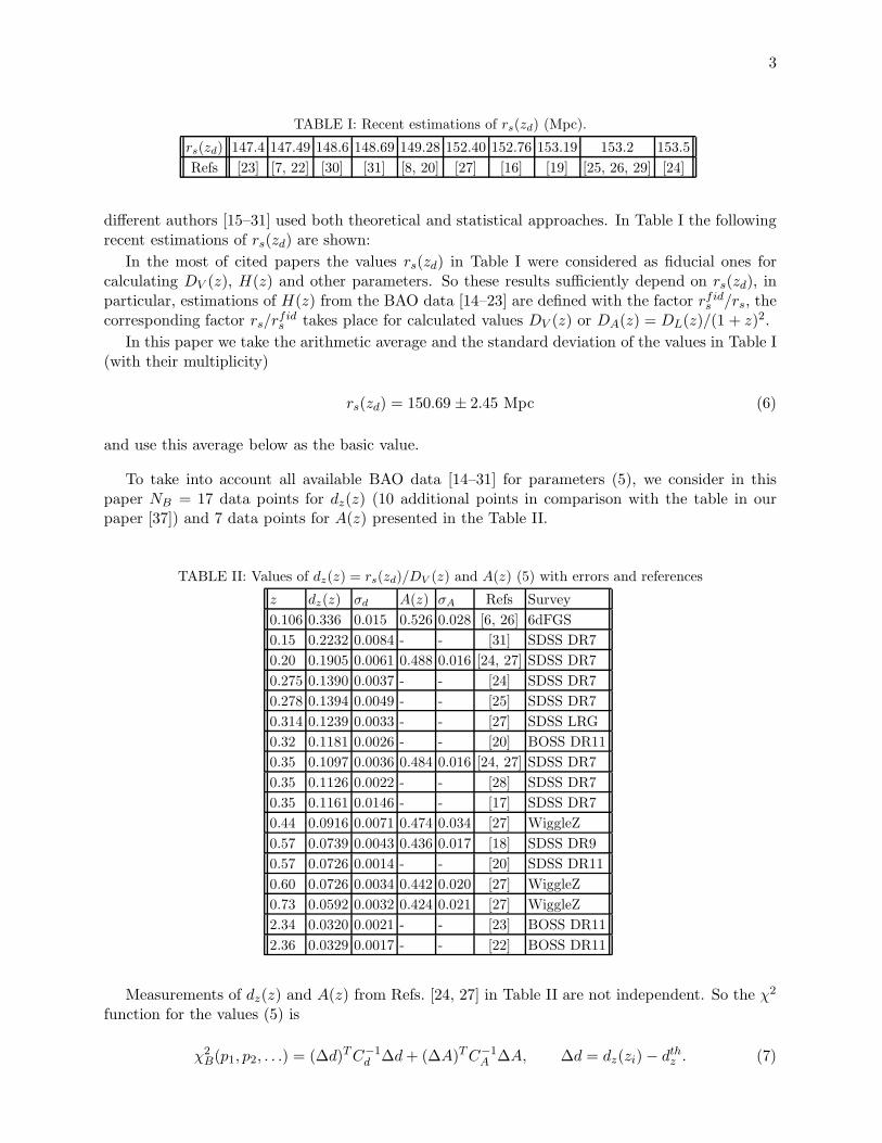
TABLE I: Recent estimations of rs(zd) (Mpc).

rs(zd) 147.4 147.49 148.6 148.69 149.28 152.40 152.76 153.19 153.2 153.5

Refs [23] [7, 22] [30] [31] [8, 20] [27] [16] [19] [25, 26, 29] [24]

different authors [15–31] used both theoretical and statistical approaches. In Table I the followingrecent estimations of rs(zd) are shown:

In the most of cited papers the values rs(zd) in Table I were considered as fiducial ones forcalculating DV (z), H(z) and other parameters. So these results sufficiently depend on rs(zd), inparticular, estimations of H(z) from the BAO data [14–23] are defined with the factor rfids /rs, thecorresponding factor rs/r

fids takes place for calculated values DV (z) or DA(z) = DL(z)/(1 + z)2.

In this paper we take the arithmetic average and the standard deviation of the values in Table I(with their multiplicity)

rs(zd) = 150.69 ± 2.45 Mpc (6)

and use this average below as the basic value.

To take into account all available BAO data [14–31] for parameters (5), we consider in thispaper NB = 17 data points for dz(z) (10 additional points in comparison with the table in ourpaper [37]) and 7 data points for A(z) presented in the Table II.

TABLE II: Values of dz(z) = rs(zd)/DV (z) and A(z) (5) with errors and references

z dz(z) σd A(z) σA Refs Survey

0.106 0.336 0.015 0.526 0.028 [6, 26] 6dFGS

0.15 0.2232 0.0084 - - [31] SDSS DR7

0.20 0.1905 0.0061 0.488 0.016 [24, 27] SDSS DR7

0.275 0.1390 0.0037 - - [24] SDSS DR7

0.278 0.1394 0.0049 - - [25] SDSS DR7

0.314 0.1239 0.0033 - - [27] SDSS LRG

0.32 0.1181 0.0026 - - [20] BOSS DR11

0.35 0.1097 0.0036 0.484 0.016 [24, 27] SDSS DR7

0.35 0.1126 0.0022 - - [28] SDSS DR7

0.35 0.1161 0.0146 - - [17] SDSS DR7

0.44 0.0916 0.0071 0.474 0.034 [27] WiggleZ

0.57 0.0739 0.0043 0.436 0.017 [18] SDSS DR9

0.57 0.0726 0.0014 - - [20] SDSS DR11

0.60 0.0726 0.0034 0.442 0.020 [27] WiggleZ

0.73 0.0592 0.0032 0.424 0.021 [27] WiggleZ

2.34 0.0320 0.0021 - - [23] BOSS DR11

2.36 0.0329 0.0017 - - [22] BOSS DR11

Measurements of dz(z) and A(z) from Refs. [24, 27] in Table II are not independent. So the χ2

function for the values (5) is

χ2B(p1, p2, . . .) = (∆d)TC−1

d ∆d+ (∆A)TC−1A ∆A, ∆d = dz(zi)− dthz . (7)

4

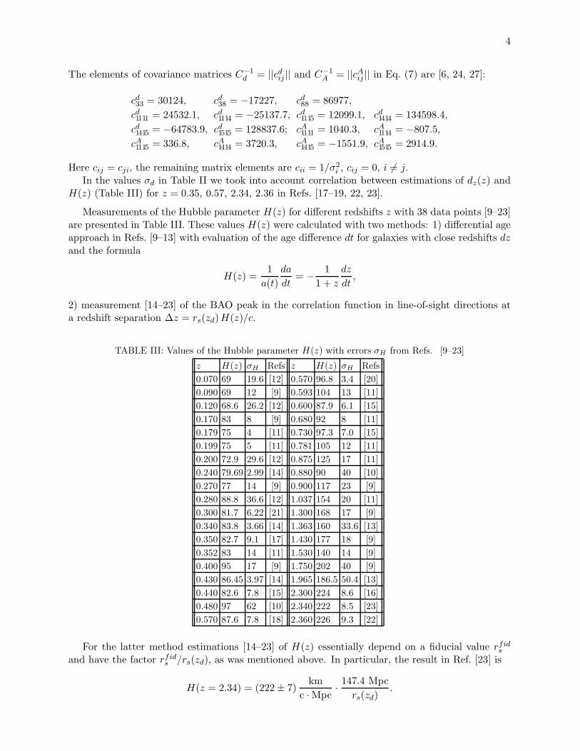
The elements of covariance matrices C−1d = ||cdij || and C−1

A = ||cAij || in Eq. (7) are [6, 24, 27]:

cd33 = 30124, cd38 = −17227, cd88 = 86977,

cd1111 = 24532.1, cd1114 = −25137.7, cd1115 = 12099.1, cd1414 = 134598.4,

cd1415 = −64783.9, cd1515 = 128837.6; cA1111 = 1040.3, cA1114 = −807.5,

cA1115 = 336.8, cA1414 = 3720.3, cA1415 = −1551.9, cA1515 = 2914.9.

Here cij = cji, the remaining matrix elements are cii = 1/σ2i , cij = 0, i 6= j.

In the values σd in Table II we took into account correlation between estimations of dz(z) andH(z) (Table III) for z = 0.35, 0.57, 2.34, 2.36 in Refs. [17–19, 22, 23].

Measurements of the Hubble parameter H(z) for different redshifts z with 38 data points [9–23]are presented in Table III. These values H(z) were calculated with two methods: 1) differential ageapproach in Refs. [9–13] with evaluation of the age difference dt for galaxies with close redshifts dzand the formula

H(z) =1

a(t)

da

dt= − 1

1 + z

dz

dt,

2) measurement [14–23] of the BAO peak in the correlation function in line-of-sight directions ata redshift separation ∆z = rs(zd)H(z)/c.

TABLE III: Values of the Hubble parameter H(z) with errors σH from Refs. [9–23]

z H(z) σH Refs z H(z) σH Refs

0.070 69 19.6 [12] 0.570 96.8 3.4 [20]

0.090 69 12 [9] 0.593 104 13 [11]

0.120 68.6 26.2 [12] 0.600 87.9 6.1 [15]

0.170 83 8 [9] 0.680 92 8 [11]

0.179 75 4 [11] 0.730 97.3 7.0 [15]

0.199 75 5 [11] 0.781 105 12 [11]

0.200 72.9 29.6 [12] 0.875 125 17 [11]

0.240 79.69 2.99 [14] 0.880 90 40 [10]

0.270 77 14 [9] 0.900 117 23 [9]

0.280 88.8 36.6 [12] 1.037 154 20 [11]

0.300 81.7 6.22 [21] 1.300 168 17 [9]

0.340 83.8 3.66 [14] 1.363 160 33.6 [13]

0.350 82.7 9.1 [17] 1.430 177 18 [9]

0.352 83 14 [11] 1.530 140 14 [9]

0.400 95 17 [9] 1.750 202 40 [9]

0.430 86.45 3.97 [14] 1.965 186.5 50.4 [13]

0.440 82.6 7.8 [15] 2.300 224 8.6 [16]

0.480 97 62 [10] 2.340 222 8.5 [23]

0.570 87.6 7.8 [18] 2.360 226 9.3 [22]

For the latter method estimations [14–23] of H(z) essentially depend on a fiducial value rfids

and have the factor rfids /rs(zd), as was mentioned above. In particular, the result in Ref. [23] is

H(z = 2.34) = (222± 7)km

c ·Mpc· 147.4 Mpc

rs(zd).

5

In Table III this factor is taken into account only for the errors σH from the papers [14, 16–18, 22, 23], where fiducial values rfids essentially differ from the average (6). The estimations forH(z) in Table III are the same as in the correspondent sources.

To compare the H(z) data in Table III with NH = 38 data points with model predictions weuse the χ2 function

χ2H(p1, p2, . . .) =

NH∑

i=1

[Hi −Hth(zi, p1, p2, . . .)]2

σ2H,i

, (8)

similar to the functions (3), (7) for the SN and BAO observational data from Ref. [3] and Table II.

III. ΛCDM MODEL

In the ΛCDM and other models considered in this paper the Einstein equations

Gµν = 8πGT µ

ν − Λδµν (9)

describe dynamics of the universe. Here Gµν = Rµ

ν − 12Rδµν ,

T µν = diag (−ρ, p, p, p). (10)

In the ΛCDM model baryonic and dark matter may be described as one component of dust-likematter with density ρ = ρc = ρb+ρdm, so we suppose p = 0 in Eq. (10). In models with Chaplygingas (Sect. IV) and with quadratic equation of state (Sect. V) we suppose that an additionalcomponent of matter describes both dark matter and dark energy and gives some contribution ρgin the total density:

ρ = ρc + ρg + ρr. (11)

The fraction of relativistic matter (radiation and neutrinos) is close to zero for observable valuesz ≤ 2.36, so below we suppose ρr = 0.

For the Robertson-Walker metric with the curvature sign k

ds2 = −dt2 + a2(t)[

(1− kr2)−1dr2 + r2dΩ]

(12)

the Einstein equations (9) are reduced to the system

3a2 + k

a2= 8πGρ+ Λ, (13)

ρ = −3a

a(ρ+ p). (14)

Eq. (14) results from the continuity condition T µν;µ = 0, the dot denotes the time derivative, here

and below the speed of light c = 1.For the ΛCDM with dust-like matter (p = 0) we use the solution of Eq. (14) ρ/ρ0 = (a/a0)

−3

and rewrite Eq. (13) in the form

a2

a2H20

=H2

H20

= Ωm

( a

a0

)−3+ΩΛ +Ωk

( a

a0

)−2. (15)

Here the present time fractions of matter, dark energy (Λ term) and curvature

Ωm =8πGρ(t0)

3H20

, ΩΛ =Λ

3H20

, Ωk = − k

a20H20

(16)

6

are connected by the equality

Ωm +ΩΛ +Ωk = 1, (17)

resulting from Eq. (15) if we fix t = t0.If we introduce dimensionless time τ and logarithm of the scale factor [36]

τ = H0t, A = loga

a0. (18)

equation (15) will take the form

dAdτ

=√

Ωme−3A +ΩΛ +Ωke−2A, (19)

more convenient for numerical solving with the initial condition at the present time A|τ=1 = 0equivalent to a(t0) = a0. Here and below the present time t = t0 corresponds to τ = 1.

If we apply the ΛCDM model for describing the observational data considered in Sect. II (forz ≤ 2.36) we use only three free model parameters, for example, H0, Ωm and ΩΛ. One can takeΩk instead of Ωm or ΩΛ.

If we fix the mentioned parameters H0, Ωm and ΩΛ, we can solve numerically the Cauchyproblem for Eq. (15) and calculate the values a(t)/a0, H(z), DL(z) (1), dz(z) and A(z) (5). Tocompare them with the observational data from Ref. [3] and Tables II, III we use the χ2 functions(3), (7) and (8) and their sum

χ2Σ = χ2

S + χ2H + χ2

B. (20)

The results of calculations are presented in Fig. 1. The top-left panel illustrates how theminimum of the sum (20) minχ2

Σ = minΩm,ΩΛ

χ2Σ(H0) depend on the Hubble constant H0 (the blue

thick line). This minimum is calculated for each fixed value H0. We also show in this panel thefraction χ2

S (the black dashed line) in minχ2Σ(H0).

One may conclude that the dependence of minχ2Σ(H0) is significant. This function has the

distinct minimum at H0 ≃ 70.13 km c−1Mpc−1 and the following optimal parameters (Ωk fromEq. (17)):

ΛCDM : minχ2Σ = 595.85, Ωm = 0.278, ΩΛ = 0.757, Ωk = −0.036. (21)

We use the one-dimensional likelihood function LΣ(H0) ∼ exp(−χ2Σ/2) corresponding to

minΩm,ΩΛ

χ2Σ(H0) for estimating 1σ and 2σ errors

ΛCDM : H0 = 70.127 ± 0.317 (1σ)±0.639 (2σ) km (cMpc)−1 (22)

for the Hubble constant. Errors for other model parameters are calculated similarly and tabulatedin the “ ΛCDM” line of Table IV, where the ΛCDM is compared with other models:

The distinct minimum and sharp dependence of minχ2Σ on H0 is connected with the similar

dependence of the main contribution χ2S(H0) (the black dashed line) and with different behavior of

minimum points for χ2S , χ

2H and χ2

B in the Ωm,ΩΛ plane, when we change H0. Only for H0 closeto 70 km c−1Mpc−1 all these three minimum points (marked in the top-right panel of Fig. 1) areclose to each other.

The optimal value H0 (22) is in concordance with the Wilkinson Microwave Anisotropy Probe(WMAP) estimation [6] H0 = 69.7 ± 2.4 (Table V below), but is in tension with the values ofPlanck Collaboration [8] H0 = 67.8 ± 0.9, Hubble Space Telescope groop [52] H0 = 73.8 ± 2.4

7

68 70 72 74

600

650

700

χ2S

min χ2Σ

min

χ2 Σ

H0

68 70 72 74

0

0.5

1ΩΛ

Ωm

Ωk

H0

Ωk,

Ωm

, Ω

Λ

0 0.2 0.4 0.6

600

700

800

900

χ2S

minχ2Σ

Ωm

0.2 0.4 0.6 0.8

0

0.5

1 ΩΛ

h

Ωk

Ωm

0.5 1

600

650

700

750min χ2

Σ

χ2S

ΩΛ

0.5 1

−0.20

0.20.40.6 h

Ωm

Ωk

ΩΛ

0.1 0.2 0.3 0.4 0.5

0.5

0.6

0.7

0.8

0.9

1

χ2H

χ2B

χ2S H

0 = 70.13

Ωm

ΩΛ

0.24 0.26 0.28 0.3

0.7

0.75

0.8

0.85

596

615

615

615 H

0 = 70.13

χ2Σ

Ωm

ΩΛ

0.24 0.26 0.28 0.3

69.5

70

70.5

71

615

615

615

ΩΛ = 0.757

χ2Σ

Ωm

H0

0.65 0.7 0.75 0.8 0.8569

69.5

70

70.5

71

71.5

596

615

615

615

Ωm

= 0.278

χ2Σ

ΩΛ

H0

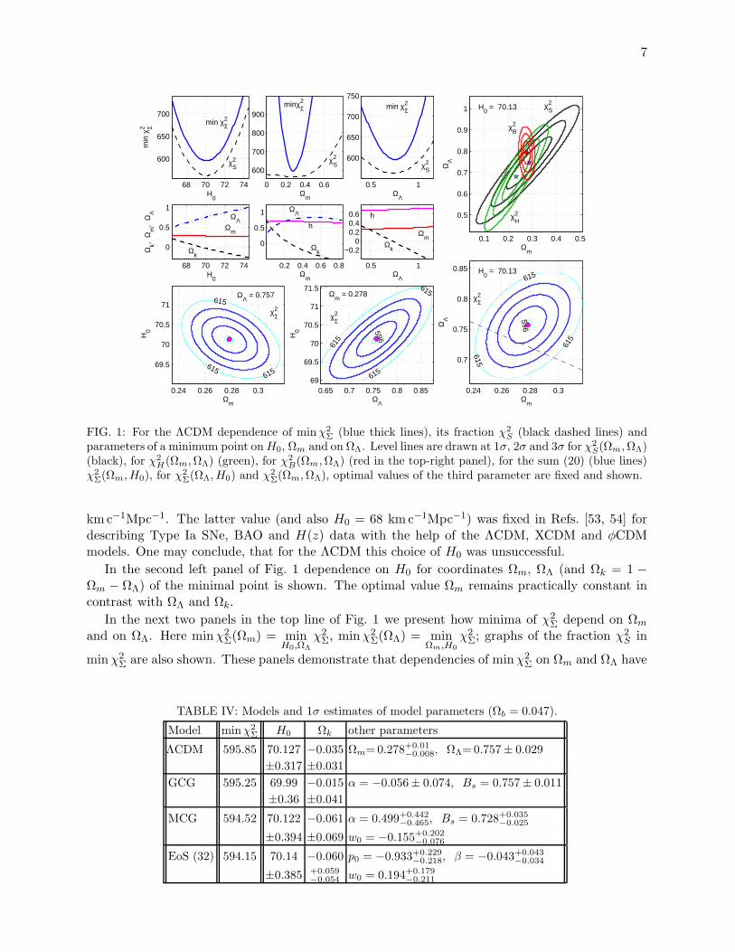
FIG. 1: For the ΛCDM dependence of minχ2Σ (blue thick lines), its fraction χ2

S (black dashed lines) andparameters of a minimum point onH0, Ωm and on ΩΛ. Level lines are drawn at 1σ, 2σ and 3σ for χ2

S(Ωm,ΩΛ)(black), for χ2

H(Ωm,ΩΛ) (green), for χ2B(Ωm,ΩΛ) (red in the top-right panel), for the sum (20) (blue lines)

χ2Σ(Ωm, H0), for χ

2Σ(ΩΛ, H0) and χ2

Σ(Ωm,ΩΛ), optimal values of the third parameter are fixed and shown.

kmc−1Mpc−1. The latter value (and also H0 = 68 kmc−1Mpc−1) was fixed in Refs. [53, 54] fordescribing Type Ia SNe, BAO and H(z) data with the help of the ΛCDM, XCDM and φCDMmodels. One may conclude, that for the ΛCDM this choice of H0 was unsuccessful.

In the second left panel of Fig. 1 dependence on H0 for coordinates Ωm, ΩΛ (and Ωk = 1 −Ωm − ΩΛ) of the minimal point is shown. The optimal value Ωm remains practically constant incontrast with ΩΛ and Ωk.

In the next two panels in the top line of Fig. 1 we present how minima of χ2Σ depend on Ωm

and on ΩΛ. Here minχ2Σ(Ωm) = min

H0,ΩΛ

χ2Σ, minχ2

Σ(ΩΛ) = minΩm,H0

χ2Σ; graphs of the fraction χ2

S in

minχ2Σ are also shown. These panels demonstrate that dependencies of minχ2

Σ on Ωm and ΩΛ have

TABLE IV: Models and 1σ estimates of model parameters (Ωb = 0.047).

Model minχ2Σ H0 Ωk other parameters

ΛCDM 595.85 70.127 −0.035 Ωm=0.278+0.01−0.008, ΩΛ=0.757± 0.029

±0.317 ±0.031

GCG 595.25 69.99 −0.015 α = −0.056± 0.074, Bs = 0.757± 0.011

±0.36 ±0.041

MCG 594.52 70.122 −0.061 α = 0.499+0.442−0.465, Bs = 0.728+0.035

−0.025

±0.394 ±0.069 w0 = −0.155+0.202−0.076

EoS (32) 594.15 70.14 −0.060 p0 = −0.933+0.229−0.218, β = −0.043+0.043

−0.034

±0.385 +0.059−0.054 w0 = 0.194+0.179

−0.211

8

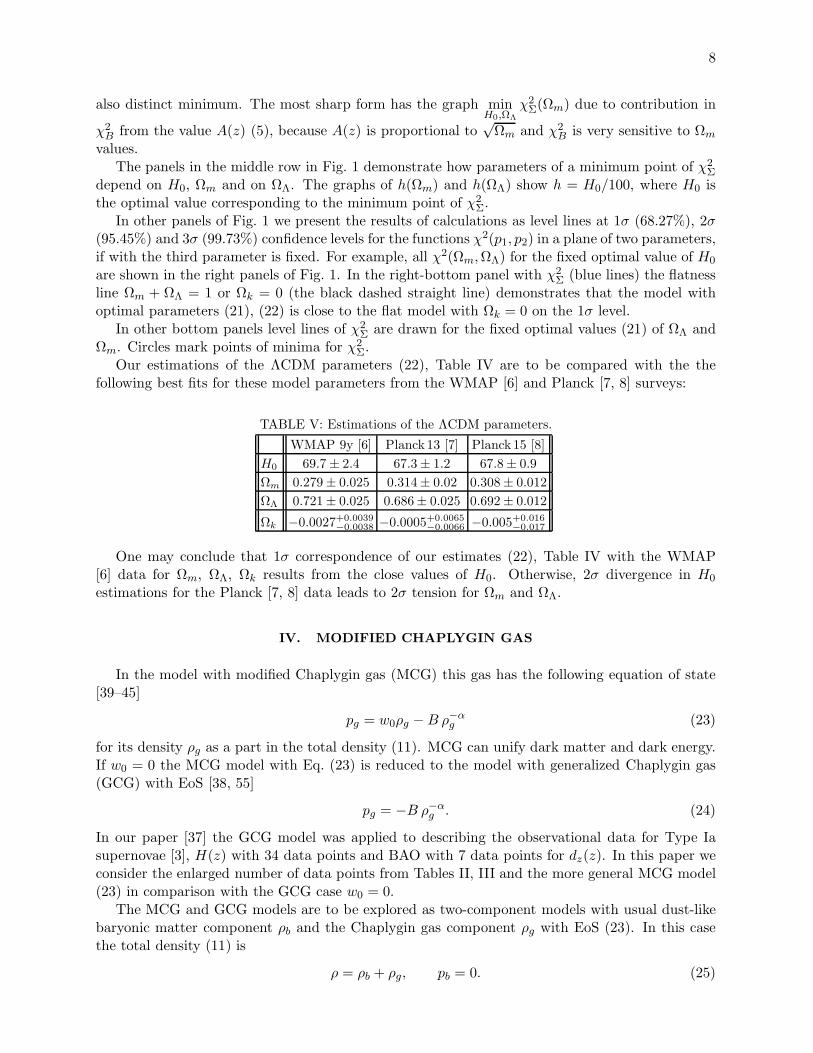
also distinct minimum. The most sharp form has the graph minH0,ΩΛ

χ2Σ(Ωm) due to contribution in

χ2B from the value A(z) (5), because A(z) is proportional to

√Ωm and χ2

B is very sensitive to Ωm

values.The panels in the middle row in Fig. 1 demonstrate how parameters of a minimum point of χ2

Σ

depend on H0, Ωm and on ΩΛ. The graphs of h(Ωm) and h(ΩΛ) show h = H0/100, where H0 isthe optimal value corresponding to the minimum point of χ2

Σ.In other panels of Fig. 1 we present the results of calculations as level lines at 1σ (68.27%), 2σ

(95.45%) and 3σ (99.73%) confidence levels for the functions χ2(p1, p2) in a plane of two parameters,if with the third parameter is fixed. For example, all χ2(Ωm,ΩΛ) for the fixed optimal value of H0

are shown in the right panels of Fig. 1. In the right-bottom panel with χ2Σ (blue lines) the flatness

line Ωm + ΩΛ = 1 or Ωk = 0 (the black dashed straight line) demonstrates that the model withoptimal parameters (21), (22) is close to the flat model with Ωk = 0 on the 1σ level.

In other bottom panels level lines of χ2Σ are drawn for the fixed optimal values (21) of ΩΛ and

Ωm. Circles mark points of minima for χ2Σ.

Our estimations of the ΛCDM parameters (22), Table IV are to be compared with the thefollowing best fits for these model parameters from the WMAP [6] and Planck [7, 8] surveys:

TABLE V: Estimations of the ΛCDM parameters.

WMAP 9y [6] Planck13 [7] Planck15 [8]

H0 69.7± 2.4 67.3± 1.2 67.8± 0.9

Ωm 0.279± 0.025 0.314± 0.02 0.308± 0.012

ΩΛ 0.721± 0.025 0.686± 0.025 0.692± 0.012

Ωk −0.0027+0.0039−0.0038 −0.0005+0.0065

−0.0066 −0.005+0.016−0.017

One may conclude that 1σ correspondence of our estimates (22), Table IV with the WMAP[6] data for Ωm, ΩΛ, Ωk results from the close values of H0. Otherwise, 2σ divergence in H0

estimations for the Planck [7, 8] data leads to 2σ tension for Ωm and ΩΛ.

IV. MODIFIED CHAPLYGIN GAS

In the model with modified Chaplygin gas (MCG) this gas has the following equation of state[39–45]

pg = w0ρg −B ρ−αg (23)

for its density ρg as a part in the total density (11). MCG can unify dark matter and dark energy.If w0 = 0 the MCG model with Eq. (23) is reduced to the model with generalized Chaplygin gas(GCG) with EoS [38, 55]

pg = −B ρ−αg . (24)

In our paper [37] the GCG model was applied to describing the observational data for Type Iasupernovae [3], H(z) with 34 data points and BAO with 7 data points for dz(z). In this paper weconsider the enlarged number of data points from Tables II, III and the more general MCG model(23) in comparison with the GCG case w0 = 0.

The MCG and GCG models are to be explored as two-component models with usual dust-likebaryonic matter component ρb and the Chaplygin gas component ρg with EoS (23). In this casethe total density (11) is

ρ = ρb + ρg, pb = 0. (25)

9

However the first component ρb and the corresponding fraction

Ωb =ρb(t0)

ρcr=

8πGρb(t0)

3H20

(26)

may include not only visible baryonic matter but also a part of cold dark matter with ρ = ρdm.Our practical applications of these models [37] demonstrated rather weak dependence of minχ2

Σ

on Ωb, so we could not separate a fraction of dark matter in ρb and did not use Ωb as an usual freeparameter of the theory.

Equation (14) for the MCG model (23) is integrable, so the analog of Eq. (15) for this model is[39–45]

H2

H20

= Ωb

( a

a0

)−3+Ωk

( a

a0

)−2+ (1− Ωb − Ωk)

[

Bs + (1−Bs)( a

a0

)−3(1+w0)(1+α)]1/(1+α)

. (27)

Here the dimensionless parameter Bs = Bρ−1−α0 /(1 +w0) is used instead of B. Thus in the MCG

model (23) we have 6 independent parameters: H0, Ωb, Ωk, w0, α and Bs. Naturally, the GCGmodel has 5 parameters: the same set without w0.

In the MCG model the parameter Ωm from its formal definition (16) equals Ωm = 1 − Ωk inaccordance with ΩΛ = 0 and Eq. (17). However, the expression A(z) (5) has the factor

√Ωm, so

one should use the effective value Ωeffm in any model. If we compare the early universe limit z ≫ 1

in the MCG equation (27) with the ΛCDM equation (15), we obtain the following effective value[43–45]:

Ωeffm = Ωb + (1− Ωb − Ωk)(1−Bs)

1/(1+α). (28)

But for the majority of observational data in Ref. [3] and Tables II, III redshifts are 0 < z < 1,so to describe correctly these data we have to consider the present time limit of Eq. (27). If wecompare limits of the right hand sides of Eqs. (15) and (27) at z → 0 or A → 0, we obtain anothereffective value [37]

Ωeffm = Ωb + (1− Ωb − Ωk)(1 −Bs)(1 + w0). (29)

Expressions (28) and (29) and their contributions in χ2B and χ2

Σ were compared in Ref. [37]. Inthis paper we use below Eq. (29) and its analogs for other models.

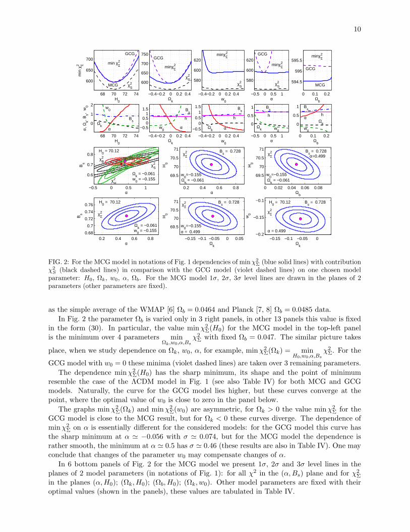
Fig. 2 shows how the MCG model (23) describes the observational data from Ref. [3] andTables II, III in comparison with the GCG model (24). Notations are the same as in Fig. 1.

In the top line panels of Fig. 2 we demonstrate how the minimums minχ2Σ of the sum (20)

for the MCG model (blue solid lines) and for the GCG model (violet dashed lines) depend on onechosen model parameter: H0, Ωk, w0, α, Ωb. These graphs determine the optimal values and errorsof the model parameters in Table IV. The second row panels of Fig. 2 correspond to panels in thetop line and present dependencies of coordinates of minima points on H0, . . ., Ωb for the MCGmodel.

In the top-right panel of Fig. 2 the value minχ2Σ for the MCG model means the minimum

over other 5 parameters for each fixed Ωb: minχ2Σ = min

H0,Ωk,w0,α,Bs

χ2Σ. Our calculations support

the previous conclusion [37] and demonstrate that the mentioned minimum minχ2Σ for the MCG

model and the corresponding minimum for the GCG model practically do not depend on Ωb in therange 0 ≤ Ωb ≤ 0.2. This behavior is connected with possible mixing of baryonic and cold darkmatter in Ωb, so, as mentioned above, we can not use Ωb as an usual free model parameter and wefix its observational value

Ωb = 0.047 (30)

10

68 70 72 74

600

650

700

χ2S

min χ2Σ

GCG

MCGm

in χ

2 Σ

H0

68 70 72 74

0

1

2

α

w0

Bs

Ωk

H0

α, Ω

k, Bs,

w0

−0.4−0.2 0 0.2 0.4

600

650

700

750GCG

χ2S

minχ2Σ

Ωk

−0.4−0.2 0 0.2 0.4

−0.50

0.51

1.5

h

α

Bs

w0

Ωk

−0.4−0.2 0 0.2 0.4

580

600

620

χ2S

minχ2Σ

w0

−0.4−0.2 0 0.2 0.4

−0.50

0.51

1.5

h

α

Bs

Ωk

w0

−0.5 0 0.5 1

580

600

620

GCG

χ2S

minχ2Σ

α

−0.5 0 0.5 1

0

0.5

1

h

w0

Bs

Ωk

α

0 0.1 0.2

594.5

595

595.5

GCG

MCG

minχ2Σ

Ωb

0 0.1 0.2

0

0.5

1

h

w0

α

Bs

Ωk

Ωb

−0.5 0 0.5 1

0.6

0.7

0.8 H

0 = 70.12

χ2H

χ2B

χ2S

Ωk = −0.061

w0 = −0.155

α

Bs

0.2 0.4 0.6 0.80.68

0.7

0.72

0.74

0.76 H

0 = 70.12

χ2Σ

α

Bs

Ωk = −0.061

w0 = −0.155

0.2 0.4 0.6 0.8

69.5

70

70.5

71 Bs = 0.728

χ2Σ

Ωk = −0.061

w0=−0.155

α

H0

−0.15 −0.1 −0.05 0 0.05

69.5

70

70.5

71

α = 0.499

χ2Σ

Bs = 0.728

w0=−0.155

Ωk

H0

0 0.02 0.04 0.06 0.08

69.5

70

70.5

71 Bs = 0.728

χ2Σ

Ωk = −0.061

w0=−0.155

Ωb

H0

α=0.499

−0.15 −0.1 −0.05 0−0.2

−0.15

−0.1 Bs = 0.728

χ2Σ

H0 = 70.12

α = 0.499

Ωk

w0

FIG. 2: For the MCG model in notations of Fig. 1 dependencies of minχ2Σ (blue solid lines) with contribution

χ2S (black dashed lines) in comparison with the GCG model (violet dashed lines) on one chosen model

parameter: H0, Ωk, w0, α, Ωb. For the MCG model 1σ, 2σ, 3σ level lines are drawn in the planes of 2parameters (other parameters are fixed).

as the simple average of the WMAP [6] Ωb = 0.0464 and Planck [7, 8] Ωb = 0.0485 data.

In Fig. 2 the parameter Ωb is varied only in 3 right panels, in other 13 panels this value is fixedin the form (30). In particular, the value minχ2

Σ(H0) for the MCG model in the top-left panelis the minimum over 4 parameters min

Ωk,w0,α,Bs

χ2Σ with fixed Ωb = 0.047. The similar picture takes

place, when we study dependence on Ωk, w0, α, for example, minχ2Σ(Ωk) = min

H0,w0,α,Bs

χ2Σ. For the

GCG model with w0 = 0 these minima (violet dashed lines) are taken over 3 remaining parameters.

The dependence minχ2Σ(H0) has the sharp minimum, its shape and the point of minimum

resemble the case of the ΛCDM model in Fig. 1 (see also Table IV) for both MCG and GCGmodels. Naturally, the curve for the GCG model lies higher, but these curves converge at thepoint, where the optimal value of w0 is close to zero in the panel below.

The graphs minχ2Σ(Ωk) and minχ2

Σ(w0) are asymmetric, for Ωk > 0 the value minχ2Σ for the

GCG model is close to the MCG result, but for Ωk < 0 these curves diverge. The dependence ofminχ2

Σ on α is essentially different for the considered models: for the GCG model this curve hasthe sharp minimum at α ≃ −0.056 with σ ≃ 0.074, but for the MCG model the dependence israther smooth, the minimum at α ≃ 0.5 has σ ≃ 0.46 (these results are also in Table IV). One mayconclude that changes of the parameter w0 may compensate changes of α.

In 6 bottom panels of Fig. 2 for the MCG model we present 1σ, 2σ and 3σ level lines in theplanes of 2 model parameters (in notations of Fig. 1): for all χ2 in the (α,Bs) plane and for χ2

Σ

in the planes (α,H0); (Ωk,H0); (Ωb,H0); (Ωk, w0). Other model parameters are fixed with theiroptimal values (shown in the panels), these values are tabulated in Table IV.

11

For the GCG model (24) these values are close to our previous estimations [37] H0 = 70.093 ±0.369, Ωk = −0.019 ± 0.045, α = −0.066+0.072

−0.074, Bs = 0.759+0.015−0.016 with 7 and 34 data points for

dz(z) and H(z) correspondingly.The results of calculation for the MCG model in Table IV should be compared with similar

results for this model in papers [43–45]. The authors of Ref. [43] for the flat model with Ωk = 0described the observational data with 557, 15 and 2 data points correspondingly for supernovae,H(z) and BAO, but they also included the cluster X-ray gas mass fraction data. Their 1σ estima-tions H0 = 70.711+4.188

−3.142 and Bs = 0.7788+0.0736−0.0723 are more wide then ours, α = 0.1079+0.3397

−0.2539 is in1σ tension, but for w0 they predict the narrow box w0 = 0.00189+0.00583

−0.00756 lying inside our estimate.In Refs. [44, 45] the MCG model with Ωk = 0 is applied for describing 12 H(z) data points, 11

points for the growth function f = d log δ/d log a of the large scale structures, 17 points for σ8(z)and also in Ref. [45] observations of supernovae and 1 data point for BAO. The authors did notdemonstrate their estimates for H0, but noted ambiguously “χ2 function for the background testis minimized by the present Hubble value predicted by WMAP7”. The best fit values of otherparameters in Ref. [45] are w0 = 0.005, α = 0.19, Bs = 0.825 with errors, calculated for pairs ofthese parameters. Only the estimate for Bs is in tension with our result in Table IV.

V. MODEL WITH QUADRATIC EQUATION OF STATE

It is interesting to compare the MCG model and the model with quadratic equation of state[46–51]

pg = p0 + w0ρg + βρ2g, (31)

because both models have 6 parameters: H0, Ωk, Ωb and 3 parameters in the EoS (23) or (31). Itis convenient to use the critical density ρcr = 3H2

0/(8πG), introduce the dimensionless parametersp0 = p0/ρcr, β = βρcr, instead of p0, β and rewrite Eq. (32) in the form

pg = p0ρcr + w0ρg + βρ2g/ρcr. (32)

Similarly to the GCG and MCG models the model with quadratic EoS (31) or (32) has theanalytical general solution of Eq. (14) in the form [48]

ρgρcr

=

12β

[

Γ−√

|∆| tan ( 32

√|∆| A)

1+|∆|−1/2 tan ( 3

2

√|∆| A)

− 1−w0

]

, ∆ < 0,

12β

[

(32A+ 1/Γ)−1 − 1− w0

]

, ∆ = 0,

ρ−(Ωm−ρ+)(a/a0)−3√

∆−ρ+(Ωm−ρ−)

(Ωm−ρ+)(a/a0)−3√

∆−Ωm+ρ−, ∆ > 0,

(33)

depending on a sign of the discriminant ∆ = (1 + w0)2 − 4βp0. Here

Ωm = 1− Ωk − Ωb, Γ = 2βΩm + 1 + w0, ρ± =−1− w0 ±

√∆

2β, A = log

a

a0.

The equation (13) for this model is reduced to the form

H2

H20

=

(

dAdτ

)2

=ρgρcr

+Ωbe−3A +Ωke

−2A. (34)

We solve this equation numerically from the present time initial condition A|τ=1 = 0 “to the past”.We can use analytical solution (33) or solve Eq. (14) numerically, these approaches are equivalent.

12

For the model (32) the effective value

Ωeffm = Ωb + p0 +Ωm(1 + w0 + βΩm) (35)

is calculated in the z → 0 or A → 0 limit similarly to the MCG model.The model with quadratic EoS (32) in the domain β > 0 may have the following singularity in

the past: when t → t∗+0 density grows to infinity, but the scale factor remains finite and nonzero:limt→t∗

ρg = ∞, limt→t∗

a = a(t∗) 6= 0. This behavior resembles the Type III finite-time future singularity

from the classification [34, 35]. In Ref. [51] the author did not see these singularities, because heconsidered only negative values β = −(w0 + 1)/ρP .

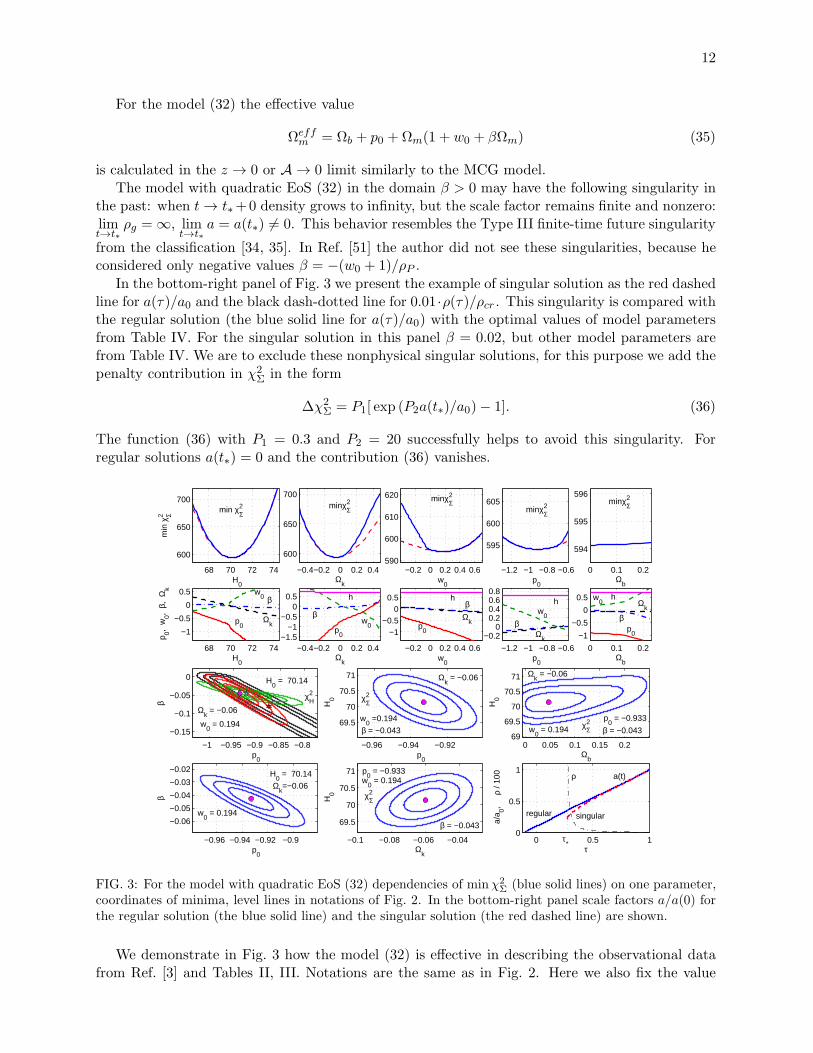
In the bottom-right panel of Fig. 3 we present the example of singular solution as the red dashedline for a(τ)/a0 and the black dash-dotted line for 0.01·ρ(τ)/ρcr . This singularity is compared withthe regular solution (the blue solid line for a(τ)/a0) with the optimal values of model parametersfrom Table IV. For the singular solution in this panel β = 0.02, but other model parameters arefrom Table IV. We are to exclude these nonphysical singular solutions, for this purpose we add thepenalty contribution in χ2

Σ in the form

∆χ2Σ = P1[ exp (P2a(t∗)/a0)− 1]. (36)

The function (36) with P1 = 0.3 and P2 = 20 successfully helps to avoid this singularity. Forregular solutions a(t∗) = 0 and the contribution (36) vanishes.

68 70 72 74

600

650

700min χ2

Σ

min

χ2 Σ

H0

68 70 72 74

−1

−0.5

0

0.5

p0

w0 β

Ωk

H0

p0,

w0,

β, Ω

k

−0.4−0.2 0 0.2 0.4

600

650

700minχ2

Σ

Ωk

−0.4−0.2 0 0.2 0.4−1.5

−1−0.5

00.5 h

p0

β w

0

Ωk

−0.2 0 0.2 0.4 0.6590

600

610

620 minχ2Σ

w0

−0.2 0 0.2 0.4 0.6

−1−0.5

00.5 h

p0

βΩ

k

w0

−1.2 −1 −0.8 −0.6

595

600

605minχ2

Σ

p0

−1.2 −1 −0.8 −0.6

−0.20

0.20.40.60.8

h w

0β

Ωk

p0

0 0.1 0.2

594

595

596minχ2

Σ

Ωb

0 0.1 0.2

−1

−0.5

0

0.5 h w0

p0

β

Ωk

Ωb

−1 −0.95 −0.9 −0.85 −0.8

−0.15

−0.1

−0.05

0 H0 = 70.14

χ2H

Ωk = −0.06

w0 = 0.194

p0

β

−0.96 −0.94 −0.92 −0.9

−0.06

−0.05

−0.04

−0.03

−0.02 H0 = 70.14

p0

β

Ωk=−0.06

w0 = 0.194

−0.96 −0.94 −0.92

69.5

70

70.5

71

β = −0.043

χ2Σ

Ωk = −0.06

w0 =0.194

p0

H0

−0.1 −0.08 −0.06 −0.04

69.5

70

70.5

71 p0 = −0.933

χ2Σ

β = −0.043

w0 = 0.194

Ωk

H0

0 0.05 0.1 0.15 0.269

69.5

70

70.5

71

β = −0.043χ2

Σ

Ωk = −0.06

w0 = 0.194

Ωb

H0

p0 = −0.933

0 0.5 10

0.5

1ρ

regular singular

a(t)

τ*

τ

a/a

0,

ρ / 1

00

FIG. 3: For the model with quadratic EoS (32) dependencies of minχ2Σ (blue solid lines) on one parameter,

coordinates of minima, level lines in notations of Fig. 2. In the bottom-right panel scale factors a/a(0) forthe regular solution (the blue solid line) and the singular solution (the red dashed line) are shown.

We demonstrate in Fig. 3 how the model (32) is effective in describing the observational datafrom Ref. [3] and Tables II, III. Notations are the same as in Fig. 2. Here we also fix the value

13

(30) Ωb = 0.047 (except for 3 right panels) and do not use Ωb as a fitting parameter, because thedependence minχ2

Σ(Ωb) = minH0,Ωk,w0,p0,β

χ2Σ (shown in the top-right panel) is rather weak.

In the top line panels of Fig. 3 we draw graphs of minχ2Σ depending on one model parameter

(H0, Ωk . . .) for the model (32) with the penalty function (36) as solid blue lines and withoutcontribution (36) as red dashed lines. In other words, for the blue lines we use only regularsolutions, for red dashed lines we also include singular solutions without physical interpretation.One can see in Fig. 3 that optimal values of model parameters (see Table IV) correspond to regularsolutions.

Minima minχ2Σ here have the same sense as in Fig. 2 for the MCG model, in particular, in

the top-left panel minχ2Σ(H0) = min

Ωk,w0,p0,βχ2Σ. Dependencies of these minima on H0 and Ωk are

distinct, for the parameters w0 and p0 they ere more smooth. These calculations and their analogfor minχ2

Σ(β) result in 1σ estimates in Table IV for the considered model.

Panels in the second row of Fig. 3 correspond the upper panels. They demonstrate evolutionof coordinates of the minimal point if we vary the chosen parameter. In 5 bottom panels minimaminχ2 depend on two model parameters (p0, β; p0,H0; Ωk,H0; Ωb,H0) when other parameters arefixed with their optimal values from Table IV. These level lines demonstrate similarity with theMCG model in Fig. 2, but for the model (32) we have alternative behavior in the (Ωk,H0) planeand more weak dependence of minχ2

Σ on Ωb in the (Ωb,H0) plane. One should emphasize thatall level lines in Fig. 3 and optimal values of the model parameters lie in the domain with regularsolutions of the quadratic EoS model (32).

VI. CONCLUSION

In this paper the Type Ia supernovae observational data from Ref. [3] and estimations of BAOparameters and H(z) from Tables II, III are described with the models ΛCDM, GCG (24), MCG(23) and the model with quadratic EoS (32). The results are tabulated in Table IV as the bestminima of the function (20) χ2

Σ and optimal values of model parameters with 1σ errors (calculatedvia one-parameter distributions).

It is interesting that predictions of different models in Table IV for their common parameters arerather close, in particular, for the models ΛCDM, MCG and with EoS (32) they areH0 = 70.13±0.4km c−1Mpc−1 and −0.13 ≤ Ωk ≤ 0.008.

The minima minχ2Σ in Table IV vary from the worst value 595.85 for the ΛCDM to the best

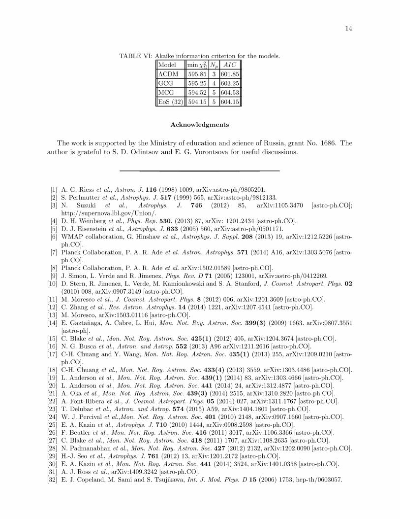
result 594.15 for the model with quadratic EoS (32). However, effectiveness of a model essentiallydepends on its number Np of model parameters (degrees of freedom). This number is used in modelselection statistics, in particular, in the following Akaike information criterion [56]

AIC = minχ2Σ + 2Np.

If we fix the value Ωb in the form (30) for the models GCG, MCG and with EoS (32) and donot use this parameter as a degrees of freedom, we will have the numbers Np and AIC for theconsidered models tabulated here in Table VI.

This information criterion adds arguments in favor of the ΛCDM model.

14

TABLE VI: Akaike information criterion for the models.

Model minχ2Σ Np AIC

ΛCDM 595.85 3 601.85

GCG 595.25 4 603.25

MCG 594.52 5 604.53

EoS (32) 594.15 5 604.15

Acknowledgments

The work is supported by the Ministry of education and science of Russia, grant No. 1686. Theauthor is grateful to S. D. Odintsov and E. G. Vorontsova for useful discussions.

[1] A. G. Riess et al., Astron. J. 116 (1998) 1009, arXiv:astro-ph/9805201.[2] S. Perlmutter et al., Astrophys. J. 517 (1999) 565, arXiv:astro-ph/9812133.[3] N. Suzuki et al., Astrophys. J. 746 (2012) 85, arXiv:1105.3470 [astro-ph.CO];

http://supernova.lbl.gov/Union/.[4] D. H. Weinberg et al., Phys. Rep. 530, (2013) 87, arXiv: 1201.2434 [astro-ph.CO].[5] D. J. Eisenstein et al., Astrophys. J. 633 (2005) 560, arXiv:astro-ph/0501171.[6] WMAP collaboration, G. Hinshaw et al., Astrophys. J. Suppl. 208 (2013) 19, arXiv:1212.5226 [astro-

ph.CO].[7] Planck Collaboration, P. A. R. Ade et al. Astron. Astrophys. 571 (2014) A16, arXiv:1303.5076 [astro-

ph.CO].[8] Planck Collaboration, P. A. R. Ade et al. arXiv:1502.01589 [astro-ph.CO].[9] J. Simon, L. Verde and R. Jimenez, Phys. Rev. D 71 (2005) 123001, arXiv:astro-ph/0412269.

[10] D. Stern, R. Jimenez, L. Verde, M. Kamionkowski and S. A. Stanford, J. Cosmol. Astropart. Phys. 02(2010) 008, arXiv:0907.3149 [astro-ph.CO].

[11] M. Moresco et al., J. Cosmol. Astropart. Phys. 8 (2012) 006, arXiv:1201.3609 [astro-ph.CO].[12] C. Zhang et al., Res. Astron. Astrophys. 14 (2014) 1221, arXiv:1207.4541 [astro-ph.CO].[13] M. Moresco, arXiv:1503.01116 [astro-ph.CO].[14] E. Gaztanaga, A. Cabre, L. Hui, Mon. Not. Roy. Astron. Soc. 399(3) (2009) 1663. arXiv:0807.3551

[astro-ph].[15] C. Blake et al., Mon. Not. Roy. Astron. Soc. 425(1) (2012) 405, arXiv:1204.3674 [astro-ph.CO].[16] N. G. Busca et al., Astron. and Astrop. 552 (2013) A96 arXiv:1211.2616 [astro-ph.CO].[17] C-H. Chuang and Y. Wang, Mon. Not. Roy. Astron. Soc. 435(1) (2013) 255, arXiv:1209.0210 [astro-

ph.CO].[18] C-H. Chuang et al., Mon. Not. Roy. Astron. Soc. 433(4) (2013) 3559, arXiv:1303.4486 [astro-ph.CO].[19] L. Anderson et al., Mon. Not. Roy. Astron. Soc. 439(1) (2014) 83, arXiv:1303.4666 [astro-ph.CO].[20] L. Anderson et al., Mon. Not. Roy. Astron. Soc. 441 (2014) 24, arXiv:1312.4877 [astro-ph.CO].[21] A. Oka et al., Mon. Not. Roy. Astron. Soc. 439(3) (2014) 2515, arXiv:1310.2820 [astro-ph.CO].[22] A. Font-Ribera et al., J. Cosmol. Astropart. Phys. 05 (2014) 027, arXiv:1311.1767 [astro-ph.CO].[23] T. Delubac et al., Astron. and Astrop. 574 (2015) A59, arXiv:1404.1801 [astro-ph.CO].[24] W. J. Percival et al.,Mon. Not. Roy. Astron. Soc. 401 (2010) 2148, arXiv:0907.1660 [astro-ph.CO].[25] E. A. Kazin et al., Astrophys. J. 710 (2010) 1444, arXiv:0908.2598 [astro-ph.CO].[26] F. Beutler et al., Mon. Not. Roy. Astron. Soc. 416 (2011) 3017, arXiv:1106.3366 [astro-ph.CO].[27] C. Blake et al., Mon. Not. Roy. Astron. Soc. 418 (2011) 1707, arXiv:1108.2635 [astro-ph.CO].[28] N. Padmanabhan et al., Mon. Not. Roy. Astron. Soc. 427 (2012) 2132, arXiv:1202.0090 [astro-ph.CO].[29] H.-J. Seo et al., Astrophys. J. 761 (2012) 13, arXiv:1201.2172 [astro-ph.CO].[30] E. A. Kazin et al., Mon. Not. Roy. Astron. Soc. 441 (2014) 3524, arXiv:1401.0358 [astro-ph.CO].[31] A. J. Ross et al., arXiv:1409.3242 [astro-ph.CO].[32] E. J. Copeland, M. Sami and S. Tsujikawa, Int. J. Mod. Phys. D 15 (2006) 1753, hep-th/0603057.

15

[33] T. Clifton, P. G. Ferreira, A. Padilla and C. Skordis, Physics Reports 513 (2012) 1, arXiv:1106.2476[astro-ph.CO].

[34] K. Bamba, S. Capozziello, S. Nojiri and S. D. Odintsov, Astrophys. and Space Science 342 (2012) 155,arXiv:1205.3421 [gr-qc].

[35] S. Nojiri and S. D. Odintsov, Phys. Rept. 505 (2011) 59, arXiv:1011.0544 [gr-qc].[36] O. A. Grigorieva and G. S. Sharov, Int. J. Mod. Phys. D 22 (2013) 1350075, arXiv:1211.4992, [gr-qc].[37] G. S. Sharov and E. G. Vorontsova, J. Cosmol. Astropart. Phys. 10 (2014) 057, arXiv:1407.5405, [gr-qc].[38] A. Y. Kamenshchik, U. Moschella and V. Pasquier, Phys. Lett. B 511(2-4) (2001) 265,

arXiv:gr-qc/0103004.[39] H. B. Benaoum, arXiv:hep-th/0205140.[40] L. P. Chimento, Phys. Rev. D. 69 (2004) 123517.[41] U. Debnath, A. Banerjee, S. Chakraborty, Class. Quant. Grav. 21 (2004) 5609, arXiv:gr-qc/0411015.[42] D-J. Liu, X-Z. Li, Chin. Phys. Lett. 22 (2005) 1600, astro-ph/0501115.[43] J. Lu, L. Xu, Y. Wu and M. Liu, Gen. Rel. Grav. 43 (2011) 819, arXiv:1105.1870 [astro-ph.CO].[44] B. C. Paul and P. Thakur, J. Cosmol. Astropart. Phys. 11 (2013) 052, arXiv:1306.4808 [astro-ph.CO].[45] B.C. Paul, P. Thakur and A. Beesham, arXiv:1410.6588 [astro-ph.CO].[46] S. Nojiri and S. D. Odintsov, Phys. Rev. D 70 (2004) 103522, arXiv:hep-th/0408170.[47] S. Nojiri, S. D. Odintsov and S. Tsujikawa, Phys. Rev. D 71 (2005) 063004, arXiv:hep-th/0501025.[48] K. N. Ananda and M. Bruni, Phys. Rev. D 74 (2006) 023523, arXiv:astro-ph/0512224.[49] E. V. Linder and R. J. Scherrer, Phys. Rev. D 80 (2009) 023008, arXiv:0811.2797 [astro-ph].[50] A. V. Astashenok, S. Nojiri, S. D. Odintsov and A. V. Yurov, Phys. Lett. B 709 (2012) 396,

arXiv:1201.4056 [gr-qc].[51] P-H. Chavanis, arXiv:1309.5784 [astro-ph.CO].[52] A. G. Riess et al., Astrophys. J. 730(2) (2011) 119, arXiv:1103.2976 [astro-ph.CO].[53] O. Farooq, D. Mania and B. Ratra, Astrophys. J. 764 (2013) 139, arXiv:1211.4253 [astro-ph.CO].[54] O. Farooq and B. Ratra, Astrophys. J. 766 (2013) L7, arXiv:1301.5243 [astro-ph.CO].[55] M. C. Bento, O. Bertolami and A. A. Sen, Phys. Rev. D 66(4) (2002) 043507, arXiv:gr-qc/0202064.[56] K. Shi, Y. F. Huang and T. Lu, Monthly Notices Roy. Astronom. Soc. 426 (2012) 2452, arXiv:1207.5875

[astro-ph.CO].