Fakultät für Physik und Geowissenschaften Physikalisches Grundpraktikum

1

O8e “Refractive Index of Gases (Rayleigh-Loewe-Interferometer)” Tasks 1. Calibrate a Rayleigh-Loewe-Interferometer with monochromatic light of known wavelength. Fit a second order polynomial to the calibration curve. 2. Determine the difference in the index of refraction Δn = n - nv of air in dependence of the gas pressure for about ten different pressure values. Plot the Δn(p) data set, determine the slope and calculate n0 (refractive index at standard conditions) for air. Express the result as refractive power β0 = (n0-1)∙106. 3. Determine the index of refraction n0 and the refractive power β0 for carbon dioxide using the same method as in task 2. Literature Physics, P. A. Tipler, 3rd Edition, Vol. 2, Chap. 33-4, 33-8, 33-3 University Physics, H. Benson, Chap. 37.3, 37.4 Physikalisches Praktikum, 13. Auflage, Hrsg. W. Schenk, F. Kremer, Optik, 2.0.2, 2.0.3, 2.2, 3.3 Accessories Laboratory interferometer after Rayleigh and Loewe, white light lamp, sodium lamp (λ = 589 nm), digital manometer, CO2 gas pressure cylinder Keywords for preparation - Interference, coherent light - Constructive and destructive interference by diffraction at a double slit - Index of refraction of gases, Lorentz-Lorenz' formula - Evaluation of the relationship between pressure and the index of refraction - Construction and operation principle of the Rayleigh-Loewe interferometer

2

Remarks The Laboratory Interferometer after Rayleigh and Loewe The laboratory interferometer uses the interference principle after Rayleigh and Löwe. A beam of light emitted by the light source passes a condensor, shines on a narrow slit and is parallelized by a collimating lens. The light is diffracted by a double slit located directly behind the collimating lens, and interference fringes are observed, when the coherence condition for spatially extended light sources is fulfilled:

tan2 2yg b

λϕ = << . (1)

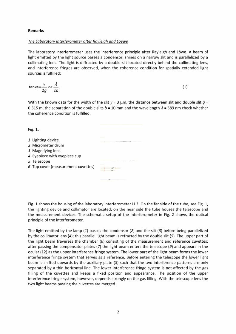
With the known data for the width of the slit y = 3 μm, the distance between slit and double slit g = 0.315 m, the separation of the double slits b = 10 mm and the wavelength λ = 589 nm check whether the coherence condition is fulfilled. Fig. 1. 1 Lighting device 2 Micrometer drum 3 Magnifying lens 4 Eyepiece with eyepiece cup 5 Telescope 6 Top cover (measurement cuvettes) Fig. 1 shows the housing of the laboratory interferometer LI 3. On the far side of the tube, see Fig. 1, the lighting device and collimator are located, on the near side the tube houses the telescope and the measurement devices. The schematic setup of the interferometer in Fig. 2 shows the optical principle of the interferometer. The light emitted by the lamp (1) passes the condensor (2) and the slit (3) before being parallelized by the collimator lens (4); this parallel light beam is refracted by the double slit (5). The upper part of the light beam traverses the chamber (6) consisting of the measurement and reference cuvettes; after passing the compensator plates (7) the light beam enters the telescope (9) and appears in the ocular (12) as the upper interference fringe system. The lower part of the light beam forms the lower interference fringe system that serves as a reference. Before entering the telescope the lower light beam is shifted upwards by the auxiliary plate (8) such that the two interference patterns are only separated by a thin horizontal line. The lower interference fringe system is not affected by the gas filling of the cuvettes and keeps a fixed position and appearance. The position of the upper interference fringe system, however, depends strongly on the gas filling. With the telescope lens the two light beams passing the cuvettes are merged.

3

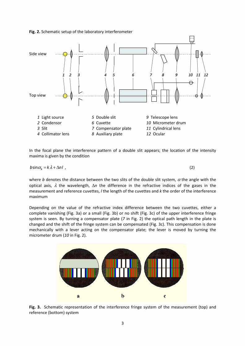
Fig. 2. Schematic setup of the laboratory interferometer Side view

Top view

1 Light source 5 Double slit 9 Telescope lens 2 Condensor 6 Cuvette 10 Micrometer drum 3 Slit 7 Compensator plate 11 Cylindrical lens 4 Collimator lens 8 Auxiliary plate 12 Ocular

In the focal plane the interference pattern of a double slit appears; the location of the intensity maxima is given by the condition

sin kb k nlα λ= + Δ , (2) where b denotes the distance between the two slits of the double slit system, α the angle with the optical axis, λ the wavelength, Δn the difference in the refractive indices of the gases in the measurement and reference cuvettes, l the length of the cuvettes and k the order of the interference maximum Depending on the value of the refractive index difference between the two cuvettes, either a complete vanishing (Fig. 3a) or a small (Fig. 3b) or no shift (Fig. 3c) of the upper interference fringe system is seen. By turning a compensator plate (7 in Fig. 2) the optical path length in the plate is changed and the shift of the fringe system can be compensated (Fig. 3c). This compensation is done mechanically with a lever acting on the compensator plate; the lever is moved by turning the micrometer drum (10 in Fig. 2). Fig. 3. Schematic representation of the interference fringe system of the measurement (top) and reference (bottom) system

4

Hints towards the experimental procedure Before starting with the measurements the tubes and cuvettes should be thoroughly flushed with the respective gas. The gas under study (air, CO2) must fill both measurement and reference cuvette. For the determination of the zero point (micrometer drum position t0) there should be atmospheric pressure in both cuvettes. Then the reference cuvette is closed to fix the number of gas molecules in the cuvette during the measurement. In case of the measurements with CO2 an analogous procedure is to be followed. Subsequently, about ten different overpressure values are generated in the measurement cuvette either with an air pump or a CO2 gas cylinder. The calibration of the interferometer should be done for the maximum measuring range tmax ≈ 3000, where t denotes the scale divisions on the micrometer drum, for shifts of five interference orders each. At the start of this measurement the zero point t0 has to be determined using white light. The calibration is made with monochromatic light (Na, λ = 589 nm). For the measurements of the pressure dependence of the refractive index again white light is used. The maximum pressure difference pmax with respect to atmospheric pressure depends on the type of gas and the cuvette length l: l = (500±0.1) mm Air: pmax= 300 mbar CO2: pmax= 200 mbar Before using the gas cylinder the demonstrator will give an introduction into the handling of gas cylinders and the valve system. The valves have to be operated carefully with two hands, where one hand supports the shaft during opening or closing of the valve. A closed valve is already open after only a few turns. After finishing the measurements the overpressure in the tubes and cuvettes has to be released. The calibration data have to be fitted with a parabola h(t) = h1 t + h2 t2 using the measured t values corrected by the zero point t0. In the experimental setup used in the undergraduate laboratory the cuvette with the movable compensator plate in front was chosen as measuring cuvette. This is arranged in such a way that the optical path length decreases with increasing values of the micrometer drum. On the theory of refractive indices in gases The refractive index of a medium is given by 0 /n c c= , where c0 is the speed of light in vacuum and c the speed of light in the substance under study. According to Maxwell’s theory of light as an electromagnetic wave the vacuum speed of light is obtained from Maxwell’s equations as

( ) 1/2

0 0 0c ε μ −= , where ε0 denotes the vacuum permittivity and μ0 the vacuum permeability. For the

speed of light in an absorption-free dielectric with relative dielectric permittivity εr and relative

permeability μr one obtains from Maxwell’s equations ( ) 1/2

r 0 r 0c ε ε μ μ −= . Most substances (except

for ferromagnets) have μr ≈ 1 and therefore 0 r/c c ε= . This yields the so-called Maxwell relation

rn ε= . For some substances εr is frequency independent in a wide frequency range from radio

waves up to visible light. Especially for air n is nearly constant in a wide frequency range. In case of CO2 there are significant deviations. This is explained by the fact that the frequency independence does only hold, when the light frequency is far from the eigenfrequencies of the atoms and molecules in the dielectric, which is obviously better fulfilled for air then for CO2. Eigenfrequencies can be taken into account by considering atoms and molecules as umdamped harmonic oscillators with various resonant frequencies. In the frequency range far away from absorption transitions one obtains the relation after Clausius and Mossotti

5

A

0

1 12 3 p

NM

ε ραε ε− =+

, (3)

where αp denotes the polarizability, ρ the density, M the molecular mass and NA Avogadro’s constant. Using Maxwell’s relation the Clausius-Mossotti equation can be rewritten as (Lorentz-Lorenz formula)

2

20

1 12 3 p

nN

nα

ε− =+

, (4)

where N = ( NA ρ / M) is the particle density. For gases at not too high pressures one has n ≈ 1, such that in Eq. (2) the approximations n2 - 1 = (n + 1)(n - 1) ≈ 2(n - 1) and n2 + 2 ≈ 3 can be made. From this one obtains the relation 1n N− ∝ at constant polarizability αp. For ideal gases one has Nρ ∝ and

2 2 1

1 1 2

p Tp T

ρρ

= ⋅ . This yields the equation

( ) ( )0 00 , ,

0

1 1 1 (1 )p T p T

T p pn n n

T p pγ ϑ− = − ⋅ ⋅ = − ⋅ ⋅ + , (5)

with which the pressure and temperature dependent refractive index np,T can be calculated for standard conditions (p0 = 1013.25 hPa, T0 =1/γ = 273.15 K, ϑ = ΔT = T-T0). The value n0 does only depend on the substance and the frequency of light. Due to the moderate change of the refractive index of gases for pressure changes, experimentally the difference in the refractive index Δn= np,T –nRef is measured, where nRef denotes the refractive index of the gas at constant pressure and constant temperature in the reference cuvette:

( ), 0 Ref0

1 ( 1)(1 )p T

pn n n

p γ ϑ∆ = − ⋅ − −

+. (6)

From the slope d(Δnp,T /dp) the value of n0 for a gas is determined.