Back-Propagation Algorithm

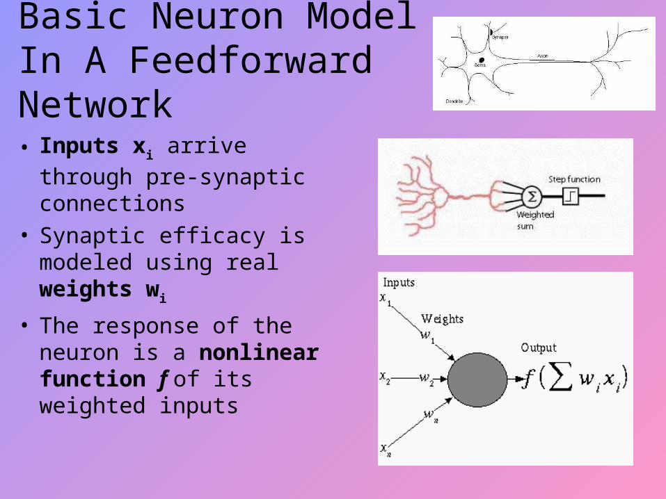
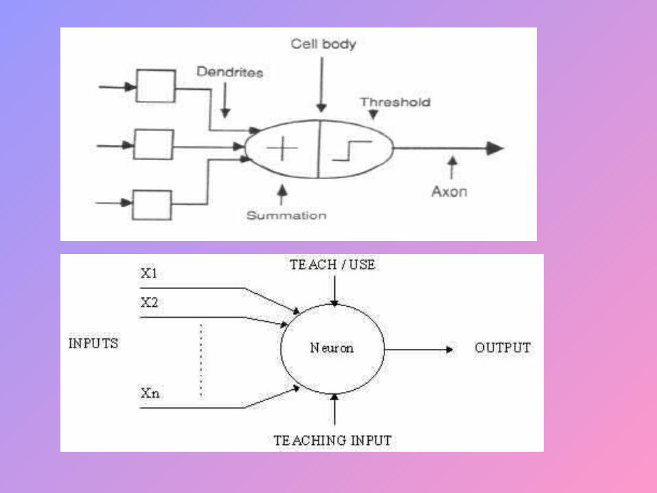
Basic Neuron Model In A Feedforward Network

• Inputs xi arrive through

pre-synaptic connections• Synaptic efficacy is

modeled using real weights wi

• The response of the neuron is a nonlinear function f of its weighted inputs

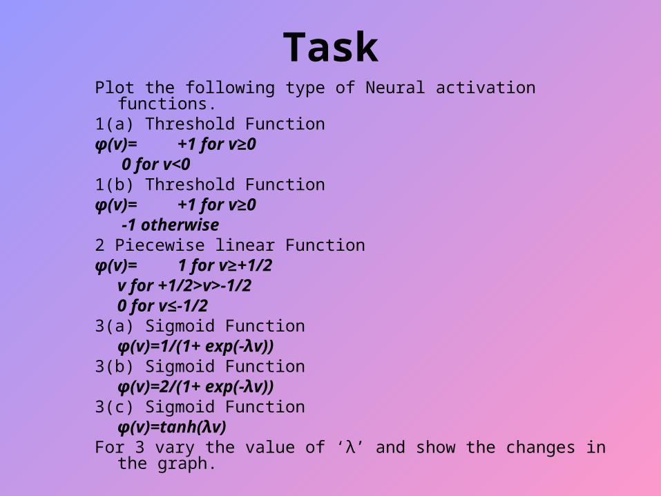
TaskPlot the following type of Neural activation functions.1(a) Threshold Functionφ(v)= +1 for v≥0

0 for v<01(b) Threshold Functionφ(v)= +1 for v≥0

-1 otherwise2 Piecewise linear Functionφ(v)= 1 for v≥+1/2

v for +1/2>v>-1/20 for v≤-1/2

3(a) Sigmoid Functionφ(v)=1/(1+ exp(-λv))

3(b) Sigmoid Functionφ(v)=2/(1+ exp(-λv))

3(c) Sigmoid Functionφ(v)=tanh(λv)

For 3 vary the value of ‘λ’ and show the changes in the graph.

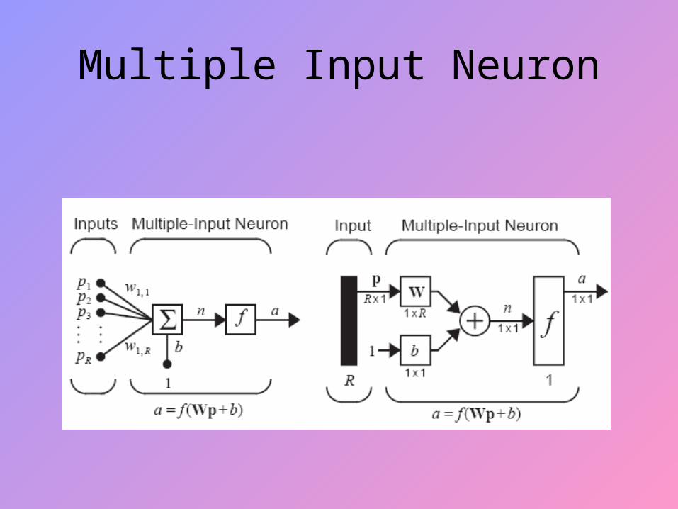
Multiple Input Neuron

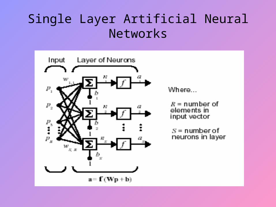
Single Layer Artificial Neural Networks

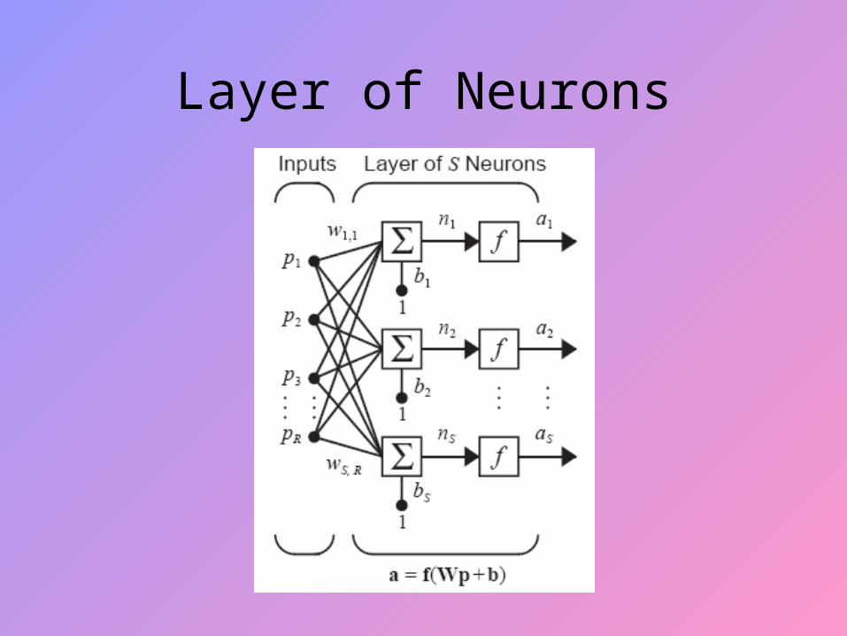
Layer of Neurons

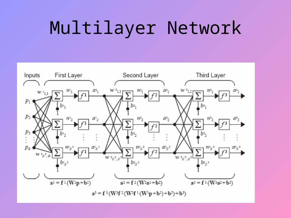
Multilayer Network

Banana & Apple Sorter

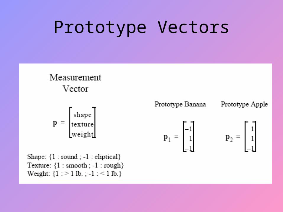
Prototype Vectors

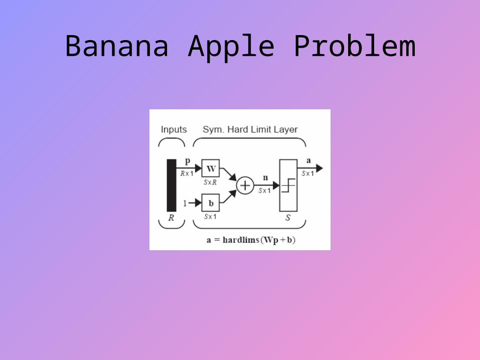
Banana Apple Problem

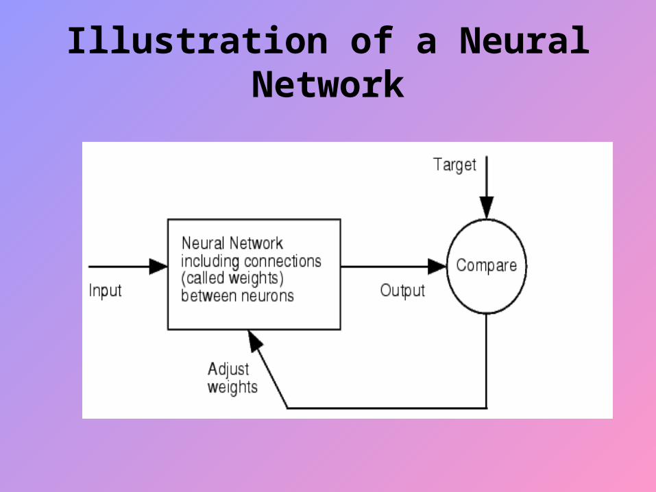
Illustration of a Neural Network

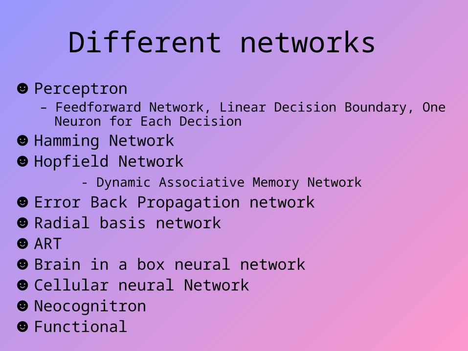
Different networks

☻Perceptron– Feedforward Network, Linear Decision Boundary, One Neuron for

Each Decision

☻Hamming Network☻Hopfield Network

- Dynamic Associative Memory Network

☻Error Back Propagation network☻Radial basis network☻ART☻Brain in a box neural network☻Cellular neural Network☻Neocognitron ☻Functional

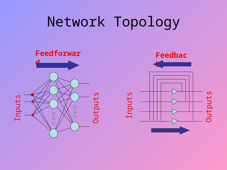
Network Topology

Feedforward

Inpu

ts

Out

puts

Inpu

ts

Feedback

Out

puts

1970s

The Backpropagation algorithm was first proposed by Paul Werbos in the 1970's. However, it was rediscoved in 1986 by Rumelhart and McClelland & became widely used.

It took 30 years before the error backpropagation (or in short: backprop) algorithm popularized.

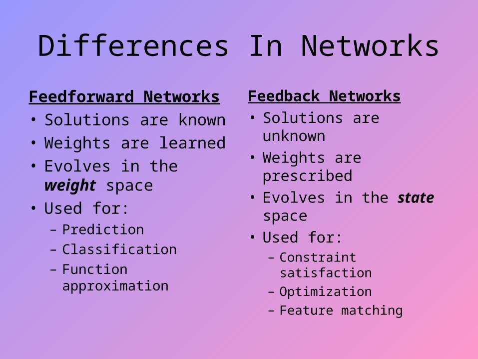
Differences In Networks

Feedforward Networks• Solutions are known• Weights are learned• Evolves in the weight

space• Used for:

– Prediction– Classification– Function

approximation

Feedback Networks• Solutions are unknown• Weights are prescribed• Evolves in the state

space• Used for:

– Constraint satisfaction– Optimization– Feature matching

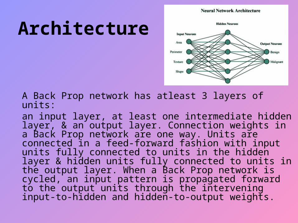
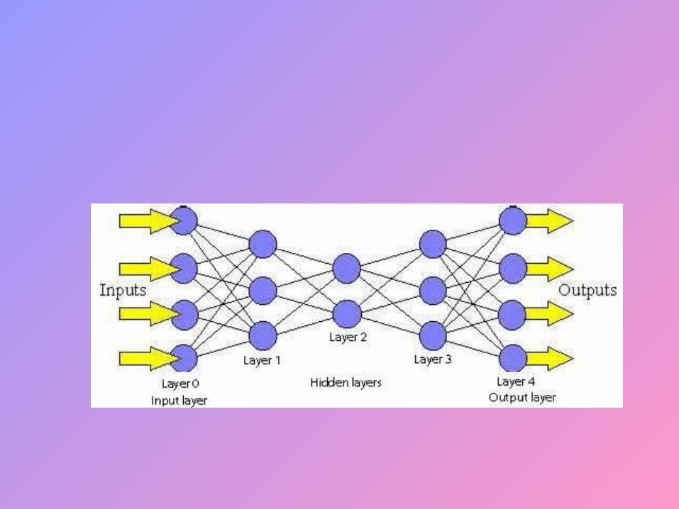
Architecture

A Back Prop network has atleast 3 layers of units: an input layer, at least one intermediate hidden layer, & an output layer. Connection weights in a Back Prop network are one way. Units are connected in a feed-forward fashion with input units fully connected to units in the hidden layer & hidden units fully connected to units in the output layer. When a Back Prop network is cycled, an input pattern is propagated forward to the output units through the intervening input-to-hidden and hidden-to-output weights.

Inputs To Neurons

• Arise from other neurons or from outside the network

• Nodes whose inputs arise outside the network are called input nodes and simply copy values

• An input may excite or inhibit the response of the neuron to which it is applied, depending upon the weight of the connection

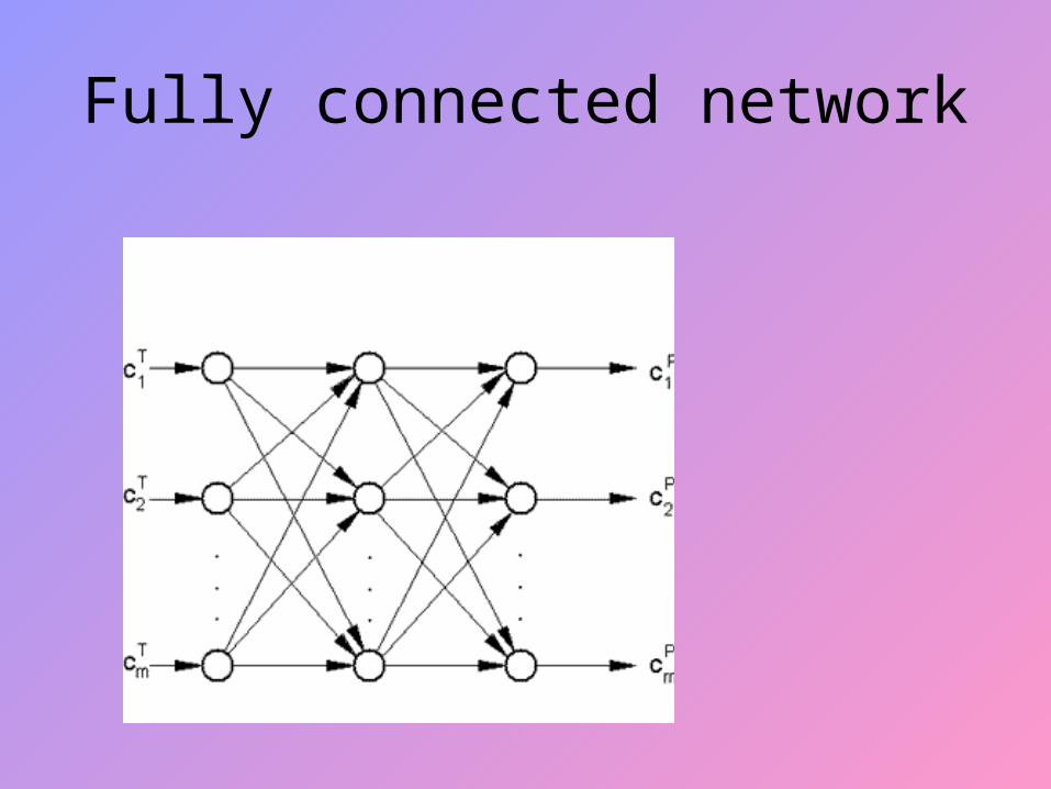
Fully connected network

Weights

• Represent synaptic efficacy and may be excitatory or inhibitory

• Normally, positive weights are considered as excitatory while negative weights are thought of as inhibitory

• Learning is the process of modifying the weights in order to produce a network that performs some function

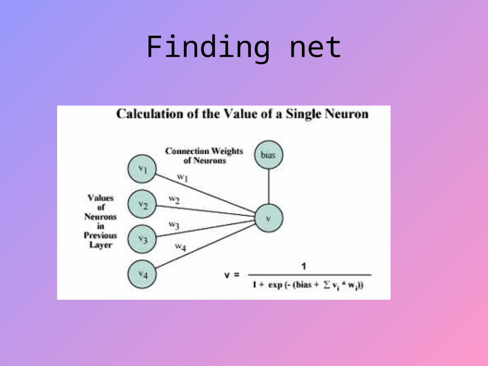
Finding net

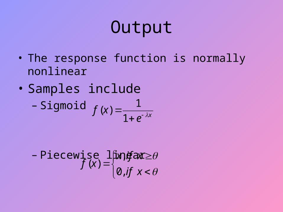
Output

• The response function is normally nonlinear

• Samples include– Sigmoid

– Piecewise linear

xexf

1

1)(

xif

xifxxf

,0

,)(

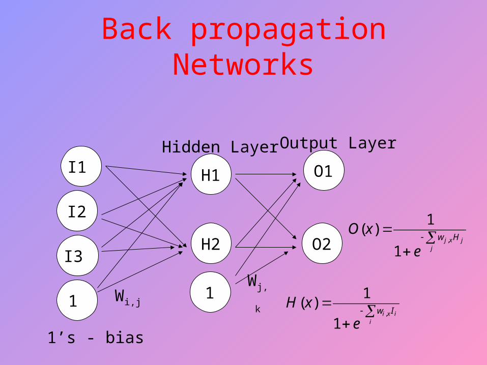
Back propagation Networks

I1

I2

1

Hidden Layer

H1

H2

O1

O2

Output Layer

Wi,jWj,k

1’s - bias

jjxj Hw

e

xO,

1

1)(

I3

1

i

ixi Iw

e

xH,

1

1)(

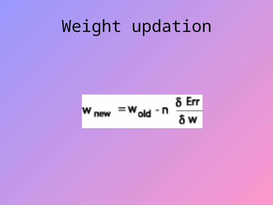
Weight updation

Backpropagation Preparation

• Training SetA collection of input-output patterns that are used to train the network

• Testing SetA collection of input-output patterns that are used to assess network performance

• Learning Rate-ηA scalar parameter, analogous to step size in numerical integration, used to set the rate of adjustments

Learning

• Learning occurs during a training phase in which each input pattern in a training set is applied to the input units and then propagated forward.

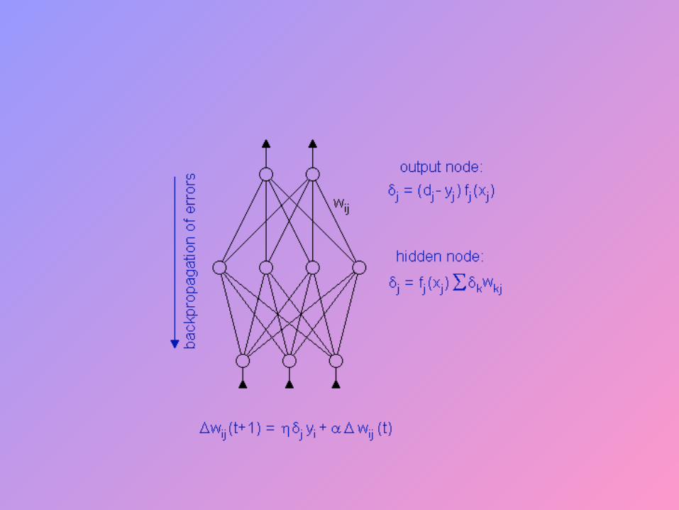
• The pattern of activation arriving at the output layer is then compared with the correct output pattern to calculate an error signal.

• The error signal for each such target output pattern is then back propagated from the outputs to the inputs in order to appropriately adjust the weights in each layer of the network.

Learning

• The process goes on for several cycles till the error reduces to a predefined limit.

• After a BackProp network has learned the correct classification for a set of inputs, it can be tested on a second set of inputs to see how well it classifies untrained patterns.

• Thus, an important consideration in applying BackProp learning is how well the network generalizes.

The basic principles of the back propagation algorithm are: (1) the error of the output signal of a neuron is used to adjust its weights such that the error decreases, and (2) the error in hidden layers is estimated proportional to the weighted sum of the (estimated) errors in the layer

above.

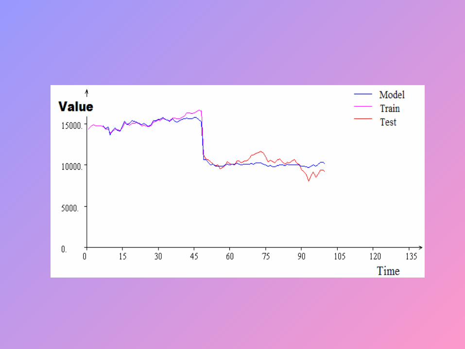
Patterns

Training patterns (70%)Testing patterns (30%)

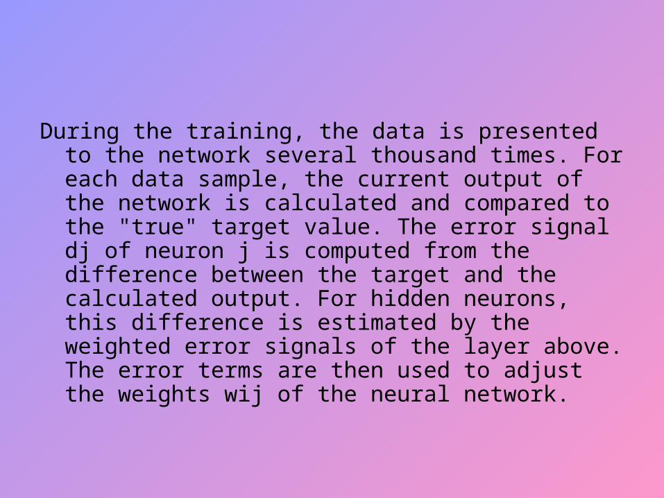
During the training, the data is presented to the network several thousand times. For each data sample, the current output of the network is calculated and compared to the "true" target value. The error signal dj of neuron j is computed from the difference between the target and the calculated output. For hidden neurons, this difference is estimated by the weighted error signals of the layer above. The error terms are then used to adjust the weights wij of the neural network.

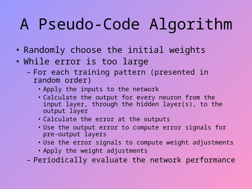
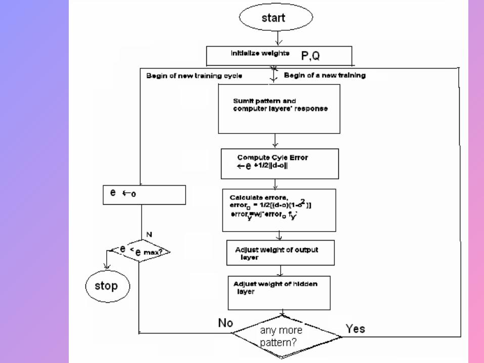
A Pseudo-Code Algorithm

• Randomly choose the initial weights• While error is too large

– For each training pattern (presented in random order)• Apply the inputs to the network• Calculate the output for every neuron from the input layer,

through the hidden layer(s), to the output layer• Calculate the error at the outputs• Use the output error to compute error signals for pre-output

layers• Use the error signals to compute weight adjustments• Apply the weight adjustments

– Periodically evaluate the network performance

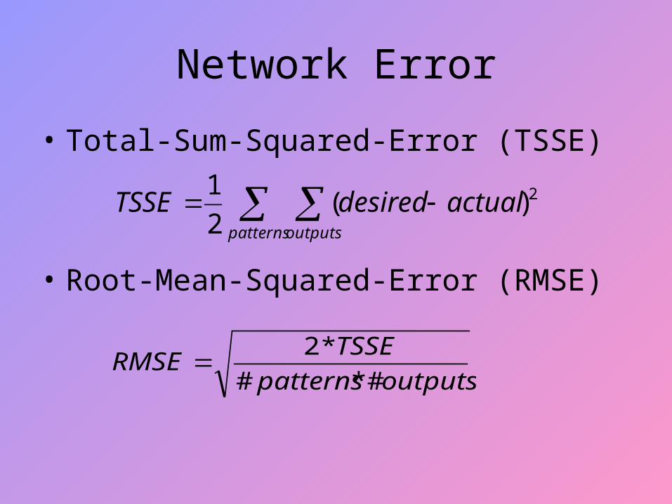
Network Error

• Total-Sum-Squared-Error (TSSE)

• Root-Mean-Squared-Error (RMSE)

patterns outputs

actualdesiredTSSE 2)(2

1

outputspatterns

TSSERMSE

*##

*2

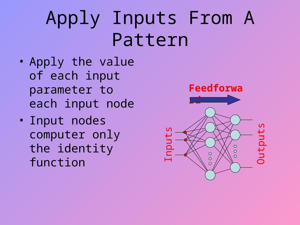
Apply Inputs From A Pattern

• Apply the value of each input parameter to each input node

• Input nodes computer only the identity function

Feedforward

Inpu

ts

Out

puts

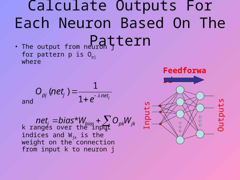
Calculate Outputs For Each Neuron Based On The Pattern

• The output from neuron j for pattern p is Opj where

and

k ranges over the input indices and Wjk is the weight on the connection from input k to neuron j

Feedforward

Inpu

ts

Out

puts

jnetjpje

netO

1

1)(

k

jkpkbiasj WOWbiasnet *

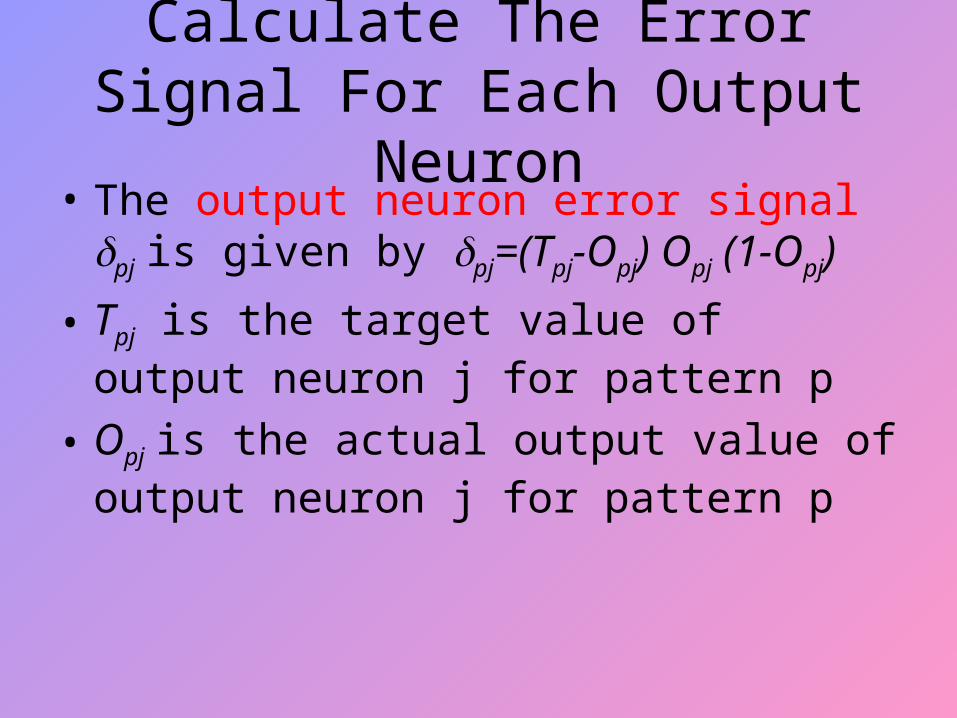
Calculate The Error Signal For Each Output Neuron

• The output neuron error signal pj is given by pj=(Tpj-Opj) Opj (1-Opj)

• Tpj is the target value of output neuron j for pattern p

• Opj is the actual output value of output neuron j for pattern p

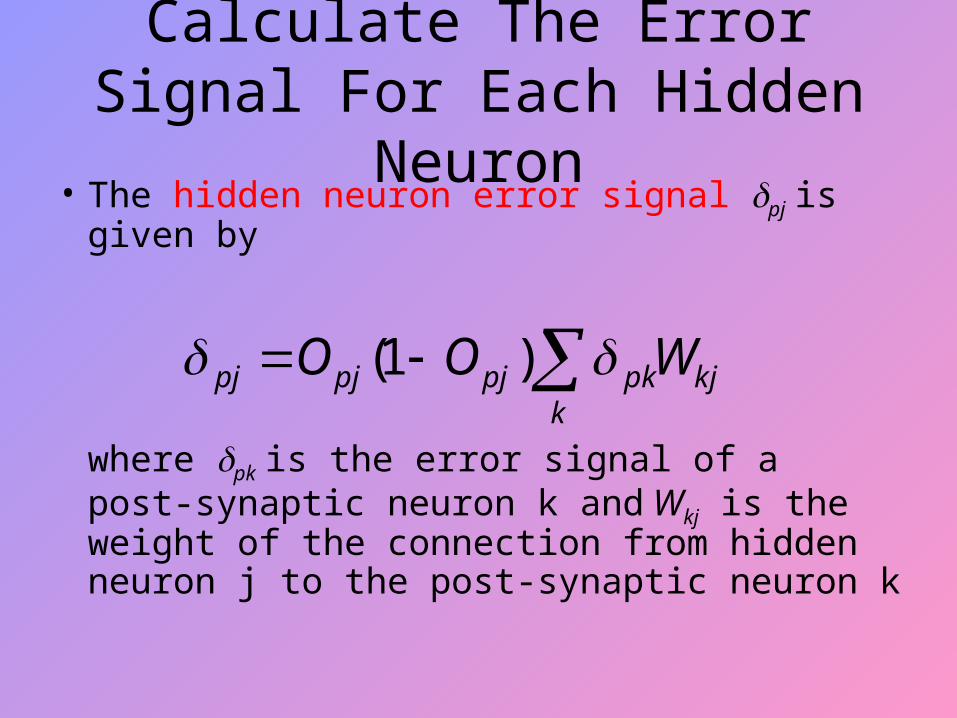
Calculate The Error Signal For Each Hidden Neuron

• The hidden neuron error signal pj is given by

where pk is the error signal of a post-synaptic neuron k and Wkj is the weight of the connection from hidden neuron j to the post-synaptic neuron k

kjk

pkpjpjpj WOO )1(

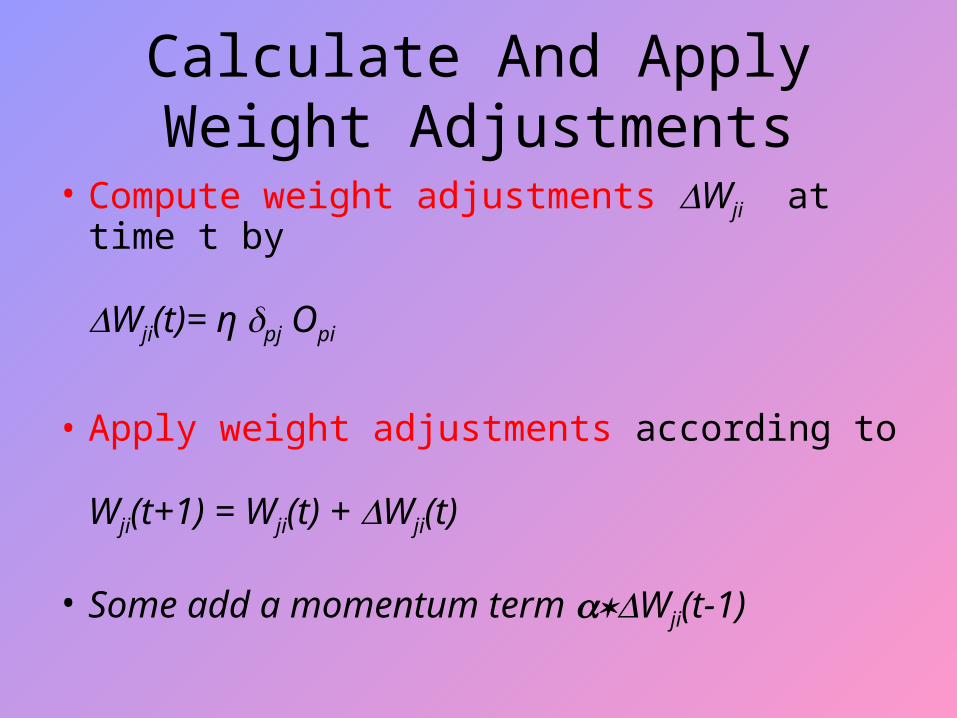
Calculate And Apply Weight Adjustments

• Compute weight adjustments Wji at time t by

Wji(t)= η pj Opi

• Apply weight adjustments according to

Wji(t+1) = Wji(t) + Wji(t)

• Some add a momentum term Wji(t-1)

• Thus, the network adjusts its weights after each data sample. This learning process is in fact a gradient descent in the error surface of the weight space - with all its drawbacks. The learning algorithm is slow and prone

to getting stuck in a local minimum.

Simulation Issues

How to Select Initial Weights

Local Minima

Solutions to Local minima

Rate of Learning

Stopping Criterion

Initialization

• For the standard back propagation algorithm, the initial weights of the multi-layer perceptron have to be relatively small. They can, for instance, be selected randomly from a small interval around zero. During training they are slowly adapted. Starting with small weights is crucial, because large weights are rigid and cannot be changed quickly.

Sequential & Batch modes

For a given training set ,back-propagation learning proceeds in two basic ways:

1. Sequential Mode

2. Batch Mode

Sequential mode• The sequential mode of back-propagation learning is also

referred to as on-line, pattern or stochastic mode.• To be specific, consider an epoch consisting of N training

ex. Arranged in the order (x(1),d(1)),…,(x(N),d(N)).

• The first ex. pair (x(1),d(1))in the epoch is presented to the network,& the sequence of forward & backward computations described previously is performed, resulting in certain adjustments to the synaptic weights & bias level of the network.

• The second ex. (x(N),d(N)) in the epoch is presented,& the sequence of forward & backward computations is repeated, resulting in the further adjustments to the synaptic weights & bias levels. This process is continued until the last example pair (x(N),d(N)) in the epoch is accounted for.

Batch Propagation

• In this mode of back-propagation learning weight updating is performed after the presentation of all the training examples that constitute an epoch.

• For a particular epoch, the cost function is the average squared error, reproduced here in composite form is defined as:-

ξav = (1/2N )Σ Σ ej2(n) for n=1 to N

for j € C

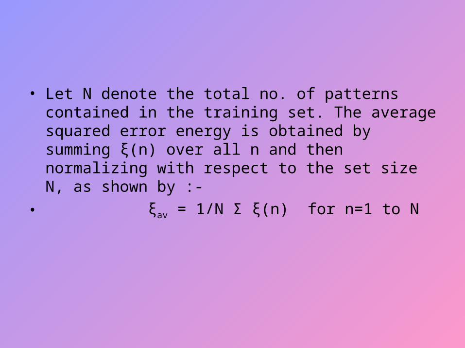
• Let N denote the total no. of patterns contained in the training set. The average squared error energy is obtained by summing ξ(n) over all n and then normalizing with respect to the set size N, as shown by :-

• ξav = 1/N Σ ξ(n) for n=1 to N

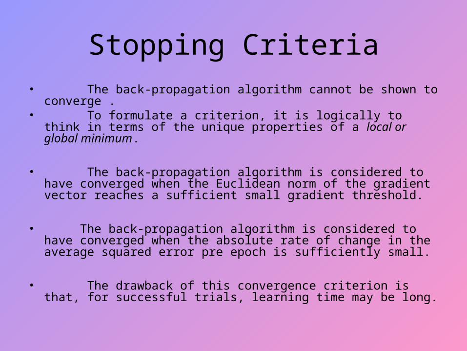
Stopping Criteria• The back-propagation algorithm cannot be shown to

converge .• To formulate a criterion, it is logically to think in terms of the

unique properties of a local or global minimum.

• The back-propagation algorithm is considered to have converged when the Euclidean norm of the gradient vector reaches a sufficient small gradient threshold.

• The back-propagation algorithm is considered to have converged when the absolute rate of change in the average squared error pre epoch is sufficiently small.

• The drawback of this convergence criterion is that, for successful trials, learning time may be long.

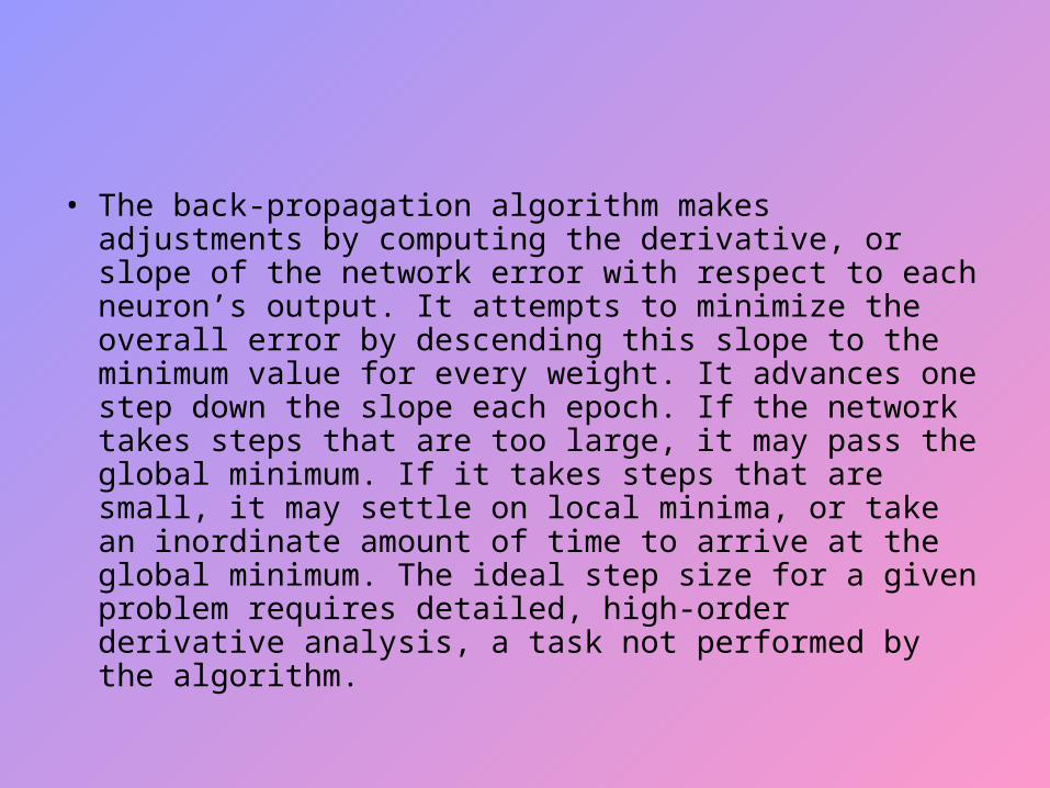
• The back-propagation algorithm makes adjustments by computing the derivative, or slope of the network error with respect to each neuron’s output. It attempts to minimize the overall error by descending this slope to the minimum value for every weight. It advances one step down the slope each epoch. If the network takes steps that are too large, it may pass the global minimum. If it takes steps that are small, it may settle on local minima, or take an inordinate amount of time to arrive at the global minimum. The ideal step size for a given problem requires detailed, high-order derivative analysis, a task not performed by the algorithm.

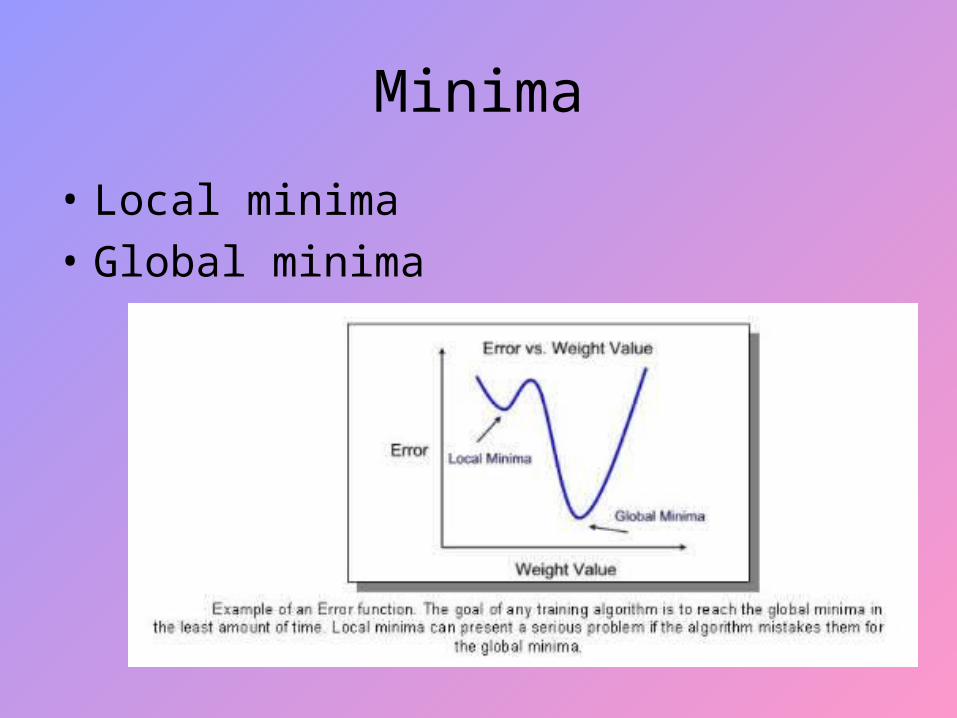
Minima

• Local minima

• Global minima

Local Minima

For simple 2 layer networks (without a hidden layer), the error surface is bowl shaped and using gradient-descent to minimize error is not a problem; the network will always find an errorless solution (at the bottom of the bowl). Such errorless solutions are called global minima.

However, extra hidden layer implies complex surfaces. Since some minima are deeper than others, it is possible that gradient descent may not find a global minima. Instead, the network may fall into local minima which represent suboptimal solutions.

• The algorithm cycles through the training samples as:-• Initialization• Presentation of training Examples• Forward Computation

Initialization

• Assuming that no prior information is available, pick the synaptic weights and thresholds from a uniform distribution whose mean is zero & whose variance is chosen to make the standard deviation of the induced local fields of the neurons lie at the transition between the linear and saturated parts of the sigmoid activation function.

Presentation of training Examples

Present the network with an epoch of training examples. For each example in the set order in same fashion, perform the sequence of forward and backward computation as described below.

Solutions to Local minima

Usual solution : More hidden layers. Logic - Although additional hidden units increase the complexity of the error surface, the extra dimensionalilty increases the number of possible escape routes.

Our solution – Tunneling

Rate of Learning

If the learning rate η is very small, then the algorithm proceeds slowly, but accurately follows the path of steepest descent in weight space. If η is large, the algorithm may oscillate.

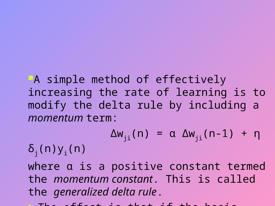
A simple method of effectively increasing the rate of learning is to modify the delta rule by including a momentum term:

Δwji(n) = α Δwji(n-1) + η δj(n)yi(n)

where α is a positive constant termed the momentum constant. This is called the generalized delta rule. The effect is that if the basic delta rule is consistently pushing a weight in the same direction, then it gradually gathers "momentum" in that direction.

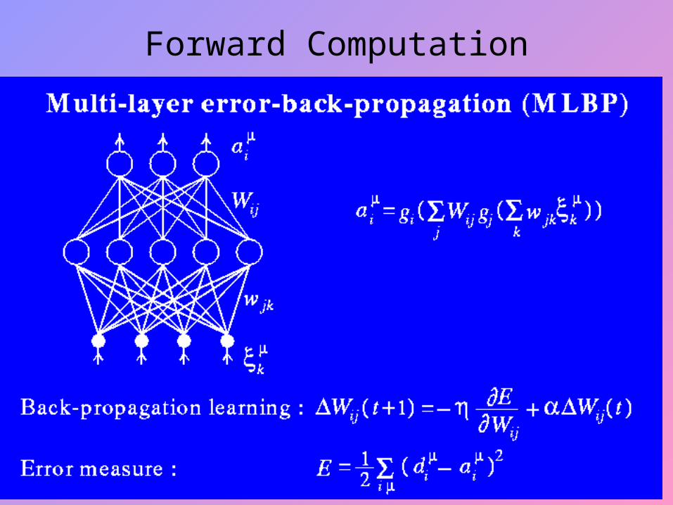
Forward Computation

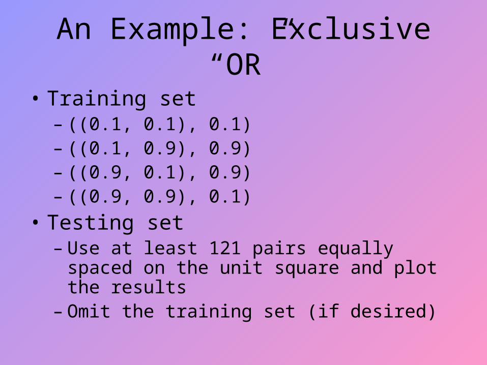
An Example: Exclusive “OR”

• Training set – ((0.1, 0.1), 0.1)– ((0.1, 0.9), 0.9)– ((0.9, 0.1), 0.9)– ((0.9, 0.9), 0.1)

• Testing set– Use at least 121 pairs equally spaced on the

unit square and plot the results– Omit the training set (if desired)

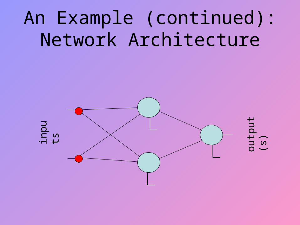
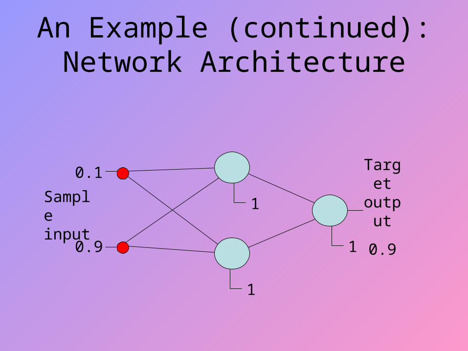
An Example (continued): Network Architecture

inpu

ts

outp

ut(s

)

An Example (continued): Network Architecture

Sample input

0.1

0.9

Target output

0.91

1

1

Feedforward Network Training by Backpropagation: Process

Summary• Select an architecture• Randomly initialize weights• While error is too large

– Select training pattern and feedforward to find actual network output

– Calculate errors and backpropagate error signals

– Adjust weights

• Evaluate performance using the test set

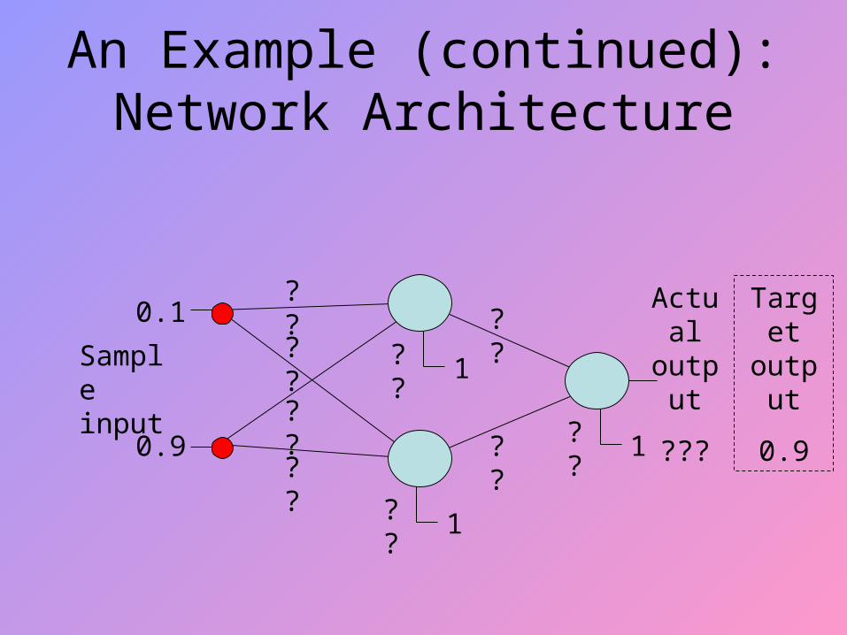
An Example (continued): Network Architecture

Sample input

0.1

0.9

Actual output

???1

1

1

??

??

??

??

??

??

??

?? ??

Target output

0.9

Feedforward Network Training by Backpropagation: Process

Summary• Select an architecture• Randomly initialize weights• While error is too large

– Select training pattern and feedforward to find actual network output

– Calculate errors and backpropagate error signals

– Adjust weights

• Evaluate performance using the test set

Backpropagation

•Very powerful - can learn any function, given enough hidden units! With enough hidden units, we can generate any function.•Have the same problems of Generalization vs. Memorization. With too many units, we will tend to memorize the input and not generalize well. Some schemes exist to “prune” the neural network.

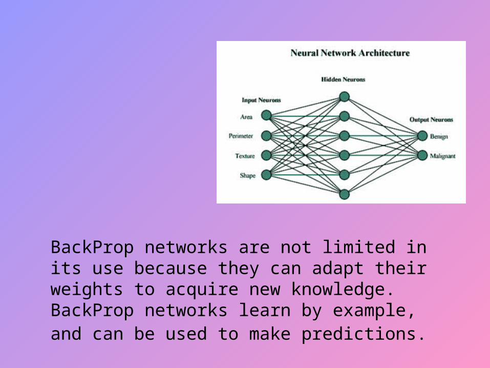
BackProp networks are not limited in its use because they can adapt their weights to acquire new knowledge. BackProp networks learn by example, and can be used to make predictions.

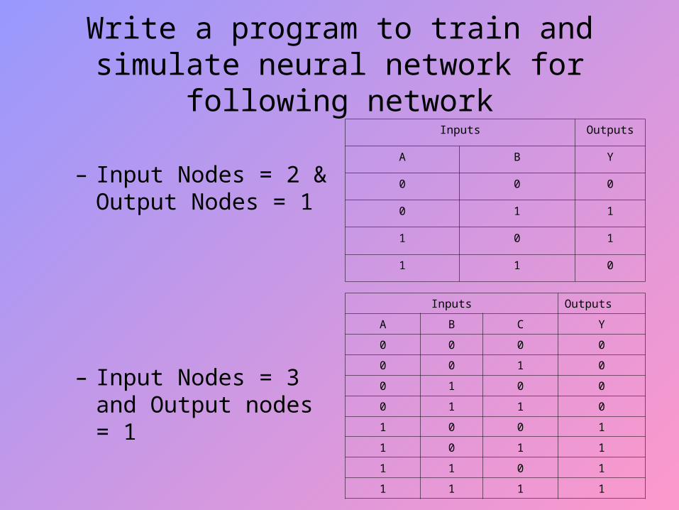
Write a program to train and simulate neural network for following network

– Input Nodes = 2 & Output Nodes = 1

– Input Nodes = 3 and Output nodes = 1

Inputs Outputs

A B Y

0 0 0

0 1 1

1 0 1

1 1 0

Inputs Outputs

A B C Y

0 0 0 0

0 0 1 0

0 1 0 0

0 1 1 0

1 0 0 1

1 0 1 1

1 1 0 1

1 1 1 1

• Artificial Neural Network – Simon Haykin

• Artificial Neural Network – Jacek Zurada