Numerical Solutions to Partial Differential Equations · 2018-11-24 · Numerical Solutions to...
34
Numerical Solutions to Partial Differential Equations Zhiping Li LMAM and School of Mathematical Sciences Peking University
Transcript of Numerical Solutions to Partial Differential Equations · 2018-11-24 · Numerical Solutions to...
Numerical Solutions toPartial Differential Equations
Zhiping Li
LMAM and School of Mathematical SciencesPeking University
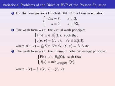
Variational Problems of the Dirichlet BVP of the Poisson Equation
1 For the homogeneous Dirichlet BVP of the Poisson equation−4u = f , x ∈ Ω,
u = 0, x ∈ ∂Ω,
2 The weak form w.r.t. the virtual work principle:Find u ∈ H1
0(Ω), such that
a(u, v) = (f , v), ∀v ∈ H10(Ω),
where a(u, v) =∫
Ω∇u · ∇v dx , (f , v) =∫
Ω fv dx .
3 The weak form w.r.t. the minimum potential energy principle:Find u ∈ H1
0(Ω), such that
J(u) = minv∈H10(Ω) J(v),
where J(v) = 12 a(v , v)− (f , v).
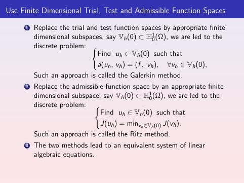
Use Finite Dimensional Trial, Test and Admissible Function Spaces
1 Replace the trial and test function spaces by appropriate finitedimensional subspaces, say Vh(0) ⊂ H1
0(Ω), we are led to thediscrete problem:
Find uh ∈ Vh(0) such that
a(uh, vh) = (f , vh), ∀vh ∈ Vh(0),
Such an approach is called the Galerkin method.
2 Replace the admissible function space by an appropriate finitedimensional subspace, say Vh(0) ⊂ H1
0(Ω), we are led to thediscrete problem:
Find uh ∈ Vh(0) such that
J(uh) = minvh∈Vh(0) J(vh).
Such an approach is called the Ritz method.
3 The two methods lead to an equivalent system of linearalgebraic equations.
Finite Element Methods for Elliptic Problems
Galerkin Method and Ritz Method
Algebraic Equations of the Galerkin and Ritz Methods
Derivation of Algebraic Equations of the Galerkin Method
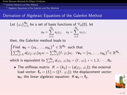
Let ϕiNhi=1 be a set of basis functions of Vh(0), let
uh =
Nh∑j=1
ujϕj , vh =
Nh∑i=1
viϕi ,
then, the Galerkin method leads toFind uh = (u1, . . . , uNh
)T ∈ RNh such that∑Nhi ,j=1 a(ϕj , ϕi )ujvi =
∑Nhi=1(f , ϕi )vi , ∀vh = (v1, . . . , vNh
)T∈ RNh ,
which is equivalent to∑Nh
j=1 a(ϕj , ϕi )uj = (f , ϕi ), i = 1, 2, · · · ,Nh.
The stiffness matrix: K = (kij) = (a(ϕj , ϕi )); the externalload vector: fh = (fi ) = ((f , ϕi )); the displacement vector:uh; the linear algebraic equation: K uh = fh.
4 / 34
Finite Element Methods for Elliptic Problems
Galerkin Method and Ritz Method
Algebraic Equations of the Galerkin and Ritz Methods
Derivation of Algebraic Equations of the Ritz Method
1 The Ritz method leads to a finite dimensional minimizationproblem, whose stationary points satisfy the equation given bythe Galerkin method, and vice versa.
2 It follows from the symmetry of a(·, ·) and the Poincare-Friedrichs inequality (see Theorem 5.4) that stiffness matrix Kis a symmetric positive definite matrix, and thus the linearsystem has a unique solution, which is a minima of the Ritzproblem.
3 So, the Ritz method also leads to K uh = fh.
5 / 34
The Key Is to Construct Finite Dimensional Subspaces
There are many ways to construct finite dimensional subspaces forthe Galerkin method and Ritz method. For example
1 For Ω = (0, 1)× (0, 1), the functions
ϕmn(x , y) = sin(mπx) sin(nπy), m, n ≥ 1,
which are the complete family of the eigenfunctions ϕi∞i=1
of the corresponding eigenvalue problem−4u = λu, x ∈ Ω,
u = 0, x ∈ ∂Ω,
and form a set of basis of H10(Ω).
2 Define VN = spanϕmn : m ≤ N, n ≤ N, the correspondingnumerical method is called the spectral method.
3 Finite element method is a systematic way to constructsubspaces for more general domains.
Finite Element Methods for Elliptic Problems
Finite Element Methods
A Typical Example of the Finite Element Method
Construction of a Finite Element Function Space for H10([0, 1]2)
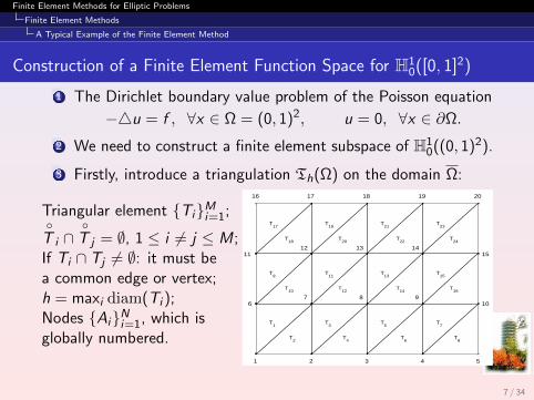
1 The Dirichlet boundary value problem of the Poisson equation
−4u = f , ∀x ∈ Ω = (0, 1)2, u = 0, ∀x ∈ ∂Ω.
2 We need to construct a finite element subspace of H10((0, 1)2).
3 Firstly, introduce a triangulation Th(Ω) on the domain Ω:
Triangular element TiMi=1;
T i ∩
T j = ∅, 1 ≤ i 6= j ≤ M;If Ti ∩ Tj 6= ∅: it must bea common edge or vertex;h = maxi diam(Ti );Nodes AiNi=1, which isglobally numbered.
1 2 3 4 5
67 8 9
10
1112 13 14
15
16 17 18 19 20
T1
T3
T5
T7
T9
T11
T13
T15
T17
T19
T21
T23
T2
T4
T6
T8
T10
T12
T14
T16
T18
T20
T22
T24
7 / 34
Finite Element Methods for Elliptic Problems
Finite Element Methods
A Typical Example of the Finite Element Method
Construction of a Finite Element Function Space for H10((0, 1)2)
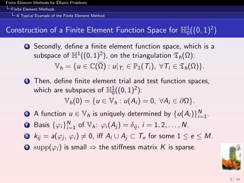
4 Secondly, define a finite element function space, which is asubspace of H1((0, 1)2), on the triangulation Th(Ω):
Vh = u ∈ C(Ω) : u|Ti∈ P1(Ti ), ∀Ti ∈ Th(Ω).
5 Then, define finite element trial and test function spaces,which are subspaces of H1
0((0, 1)2):
Vh(0) = u ∈ Vh : u(Ai ) = 0, ∀Ai ∈ ∂Ω.6 A function u ∈ Vh is uniquely determined by u(Ai )Ni=1.
7 Basis ϕiNi=1 of Vh: ϕi (Aj) = δij , i = 1, 2, . . . ,N.
8 kij = a(ϕj , ϕi ) 6= 0, iff Ai ∪ Aj ⊂ Te for some 1 ≤ e ≤ M.
9 supp(ϕi ) is small ⇒ the stiffness matrix K is sparse.
8 / 34
Finite Element Methods for Elliptic Problems
Finite Element Methods
A Typical Example of the Finite Element Method
Assemble the Global Stiffness Matrix K from the Element One K e
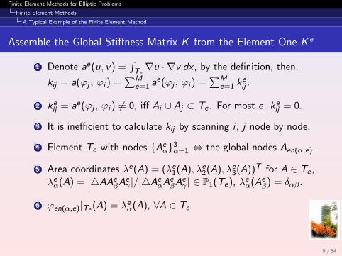
1 Denote ae(u, v) =∫Te∇u · ∇v dx , by the definition, then,
kij = a(ϕj , ϕi ) =∑M
e=1 ae(ϕj , ϕi ) =∑M
e=1 keij .
2 keij = ae(ϕj , ϕi ) 6= 0, iff Ai ∪ Aj ⊂ Te . For most e, ke
ij = 0.
3 It is inefficient to calculate kij by scanning i , j node by node.
4 Element Te with nodes Aeα3
α=1 ⇔ the global nodes Aen(α,e).
5 Area coordinates λe(A) = (λe1(A), λe2(A), λe3(A))T for A ∈ Te ,λeα(A) = |4AAe
βAeγ |/|4Ae
αAeβAe
γ | ∈ P1(Te), λeα(Aeβ) = δαβ.
6 ϕen(α,e)|Te (A) = λeα(A), ∀A ∈ Te .
9 / 34
Finite Element Methods for Elliptic Problems
Finite Element Methods
A Typical Example of the Finite Element Method
The Algorithm for Assembling Global K and fh
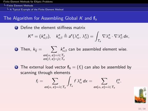
7 Define the element stiffness matrix
K e = (keαβ), ke
αβ , ae(λeα, λeβ) =
∫Te
∇λeα · ∇λeβ dx ,
8 Then, kij =∑
en(α, e)=i∈Te
en(β, e)=j∈Te
keαβ can be assembled element wise.
9 The external load vector fh = (fi ) can also be assembled byscanning through elements
fi =∑
en(α, e)=i∈Te
∫Te
f λeα dx =∑
en(α, e)=i∈Te
f eα .
10 / 34
Finite Element Methods for Elliptic Problems
Finite Element Methods
A Typical Example of the Finite Element Method
The Algorithm for Assembling Global K and fh
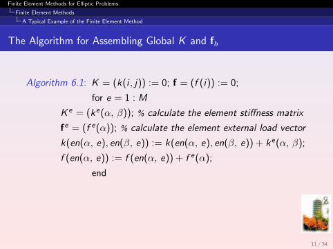
Algorithm 6.1: K = (k(i , j)) := 0; f = (f (i)) := 0;
for e = 1 : M
K e = (ke(α, β)); % calculate the element stiffness matrix
fe = (f e(α)); % calculate the element external load vector
k(en(α, e), en(β, e)) := k(en(α, e), en(β, e)) + ke(α, β);
f (en(α, e)) := f (en(α, e)) + f e(α);
end
11 / 34
Finite Element Methods for Elliptic Problems
Finite Element Methods
A Typical Example of the Finite Element Method
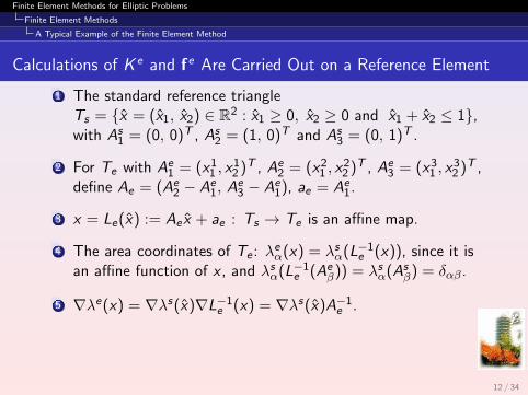
Calculations of K e and fe Are Carried Out on a Reference Element
1 The standard reference triangleTs = x = (x1, x2) ∈ R2 : x1 ≥ 0, x2 ≥ 0 and x1 + x2 ≤ 1,with As
1 = (0, 0)T , As2 = (1, 0)T and As
3 = (0, 1)T .
2 For Te with Ae1 = (x1
1 , x12 )T , Ae
2 = (x21 , x
22 )T , Ae
3 = (x31 , x
32 )T ,
define Ae = (Ae2 − Ae
1, Ae3 − Ae
1), ae = Ae1.
3 x = Le(x) := Ae x + ae : Ts → Te is an affine map.
4 The area coordinates of Te : λeα(x) = λsα(L−1e (x)), since it is
an affine function of x , and λsα(L−1e (Ae
β)) = λsα(Asβ) = δαβ.
5 ∇λe(x) = ∇λs(x)∇L−1e (x) = ∇λs(x)A−1
e .
12 / 34
Finite Element Methods for Elliptic Problems
Finite Element Methods
A Typical Example of the Finite Element Method
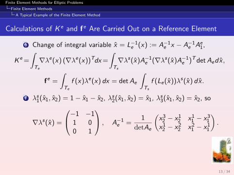
Calculations of K e and fe Are Carried Out on a Reference Element
6 Change of integral variable x = L−1e (x) := A−1
e x − A−1e Ae
1,
K e =
∫Te
∇λe(x) (∇λe(x))Tdx =
∫Ts
∇λs(x)A−1e (∇λs(x)A−1
e )Tdet Aedx ,
fe =
∫Te
f (x)λe(x) dx = det Ae
∫Ts
f (Le(x))λs(x) dx .
7 λs1(x1, x2) = 1− x1 − x2, λs2(x1, x2) = x1, λs3(x1, x2) = x2, so
∇λs(x) =
−1 −11 00 1
, A−1e =
1
detAe
(x3
2 − x12 x1
1 − x31
x12 − x2
2 x21 − x1
1
).
13 / 34

Finite Element Methods for Elliptic Problems
Finite Element Methods
A Typical Example of the Finite Element Method
Calculations of K e and fe in Terms of λs and Ae
8 The area of Ts is 1/2, hence, the element stiffness matrix is
K e =1
2 det Ae
x22 − x3
2 x31 − x2
1
x32 − x1
2 x11 − x3
1
x12 − x2
2 x21 − x1
1
(x22 − x3
2 x32 − x1
2 x12 − x2
2
x31 − x2
1 x11 − x3
1 x21 − x1
1
).
9 In general, it is necessary to apply a numerical quadrature tothe calculation of the element external load vector fe .
10 If f is a constant on Te , then
fe =1
6f (Te) det Ae (1, 1, 1)T =
1
3f (Te) |Te | (1, 1, 1)T .
14 / 34
Finite Element Methods for Elliptic Problems
Finite Element Methods
Extension to More General Boundary Conditions
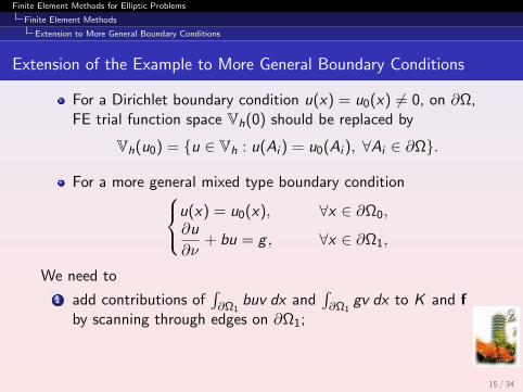
Extension of the Example to More General Boundary Conditions
For a Dirichlet boundary condition u(x) = u0(x) 6= 0, on ∂Ω,FE trial function space Vh(0) should be replaced by
Vh(u0) = u ∈ Vh : u(Ai ) = u0(Ai ), ∀Ai ∈ ∂Ω.
For a more general mixed type boundary conditionu(x) = u0(x), ∀x ∈ ∂Ω0,∂u
∂ν+ bu = g , ∀x ∈ ∂Ω1,
We need to
1 add contributions of∫∂Ω1
buv dx and∫∂Ω1
gv dx to K and fby scanning through edges on ∂Ω1;
15 / 34
Finite Element Methods for Elliptic Problems
Finite Element Methods
Extension to More General Boundary Conditions
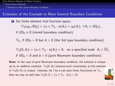
Extension of the Example to More General Boundary Conditions
2 Set finite element trial function space:
Vh(u0; ∂Ω0) = u ∈ Vh : u(Ai ) = u0(Ai ), ∀Ai ∈ ∂Ω0,
if ∂Ω0 6= ∅ (mixed boundary condition);
Vh, if ∂Ω0 = ∅ but b > 0 (the 3rd type boundary condition);
Vh(0; Ai ) = u ∈ Vh : u(Ai ) = 0, on a specified node Ai ∈ Ω,
if ∂Ω0 = ∅ and b = 0 (pure Neumann boundary condition).
Note: In the case of pure Neumann boundary condition, the solution is unique
up to an additive constant. Vh(0;Ai ) removes such uncertainty, so the solution
in Vh(0;Ai ) is unique. Likewise, let l be a non-zero linear functional on Vh,
then we may as well take Vh(0; l) = u ∈ Vh : l(u) = 0.
16 / 34
Finite Element Methods for Elliptic Problems
Finite Element Methods
Extension to More General Boundary Conditions
Summary of the Typical Example on FEM
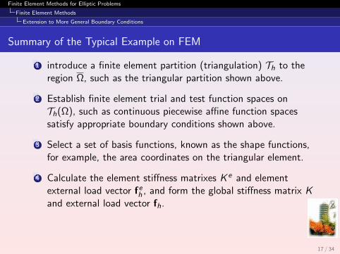
1 introduce a finite element partition (triangulation) Th to theregion Ω, such as the triangular partition shown above.
2 Establish finite element trial and test function spaces onTh(Ω), such as continuous piecewise affine function spacessatisfy appropriate boundary conditions shown above.
3 Select a set of basis functions, known as the shape functions,for example, the area coordinates on the triangular element.
4 Calculate the element stiffness matrixes K e and elementexternal load vector feh , and form the global stiffness matrix Kand external load vector fh.
17 / 34
Finite Element Methods for Elliptic Problems
Finite Element Methods
Extension to More General Boundary Conditions
Some General Remarks on the Implementation of FEM
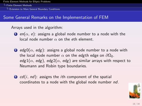
Arrays used in the algorithm:
1 en(α, e): assigns a global node number to a node with thelocal node number α on the eth element.
2 edg0(α, edg): assigns a global node number to a node withthe local node number α on the edgth edge on ∂Ω0.edg1(α, edg), edg2(α, edg) are similar arrays with respect toNeumann and Robin type boundaries.
3 cd(i , nd): assigns the ith component of the spatialcoordinates to a node with the global node number nd .
18 / 34
Finite Element Methods for Elliptic Problems
Finite Element Methods
Extension to More General Boundary Conditions
Some General Remarks on the Implementation of FEM
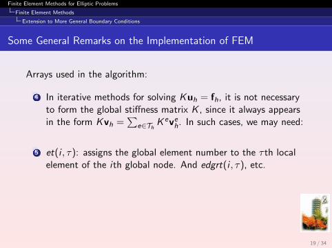
Arrays used in the algorithm:
4 In iterative methods for solving Kuh = fh, it is not necessaryto form the global stiffness matrix K , since it always appearsin the form Kvh =
∑e∈Th K eveh. In such cases, we may need:
5 et(i , τ): assigns the global element number to the τ th localelement of the ith global node. And edgrt(i , τ), etc.
19 / 34
Finite Element Methods for Elliptic Problems
Finite Element and Finite Element Function Spaces
The General Definition of Finite Element
Three Basic Ingredients in a Finite Element Function Space
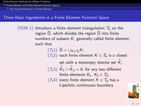
(FEM 1) Introduce a finite element triangulation Th on theregion Ω, which divides the region Ω into finitenumbers of subsets K , generally called finite element,such that
(Th1) Ω = ∪K∈ThK ;(Th2) each finite element K ∈ Th is a closed
set with a nonempty interior set
K ;
(Th3)
K 1 ∩
K 2 = ∅, for any two differentfinite elements K1, K2 ∈ Th;
(Th4) every finite element K ∈ Th has aLipschitz continuous boundary.
20 / 34
Finite Element Methods for Elliptic Problems
Finite Element and Finite Element Function Spaces
The General Definition of Finite Element
Three Basic Ingredients in a Finite Element Function Space
(FEM 2) Introduce on each finite element K ∈ Th a functionspace PK which consists of some polynomials orother functions having certain approximationproperties and at the same time easily manipulatedanalytically and numerically;
(FEM 3) The finite element function space Vh has a set of”normalized” basis functions which are easilycomputed, and each basis function has a ”small”support.
Generally speaking, a finite element is not just a subset K , itincludes also the finite dimensional function space PK defined onK and the corresponding ”normalized” basis functions.
21 / 34
Finite Element Methods for Elliptic Problems
Finite Element and Finite Element Function Spaces
The General Definition of Finite Element
General Abstract Definition of a Finite Element
Definition
A triple (K , PK , ΣK ) is called a finite element, if
1 K ⊂ Rn, called an element, is a closed set with non-emptyinterior and a Lipschitz continuous boundary;
2 PK : K → R is a finite dimensional function space consistingof sufficiently smooth functions defined on the element K ;
3 ΣK is a set of linearly independent linear functionals ϕiNi=1
defined on C∞(K ), which are called the degrees of freedom ofthe finite element and form a dual basis corresponding to a”normalized” basis of PK , meaning that there exists a uniquebasis piNi=1 of PK such that ϕi (pj) = δij .
22 / 34
Finite Element Methods for Elliptic Problems
Finite Element and Finite Element Function Spaces
The General Definition of Finite Element
An Additional Requirement on the Partition
In applications, an element K is usually taken to be
1 a triangle in R2; a tetrahedron in R3; a n simplex in Rn;
2 a rectangle or parallelogram in R2; a cuboid or a parallelepipedor more generally a convex hexahedron in R3; a parallelepipedor more generally a convex 2n polyhedron in Rn;
3 a triangle with curved edges or a tetrahedron with curvedfaces, etc..
23 / 34
Finite Element Methods for Elliptic Problems
Finite Element and Finite Element Function Spaces
The General Definition of Finite Element
An Additional Requirement on the Partition
When a region Ω is partitioned into a finite element triangulationTh with such elements, to ensure that (FEM 3) holds, the adjacentelements are required to satisfy the following compatibilitycondition:
(Th5) For any pair of K1, K2 ∈ Th, if K1⋂
K2 6= ∅, then,there must exists an 0 ≤ i ≤ n − 1, such thatK1⋂
K2 is exactly a common i dimensional face ofK1 and K2.
24 / 34
Finite Element Methods for Elliptic Problems
Finite Element and Finite Element Function Spaces
The General Definition of Finite Element
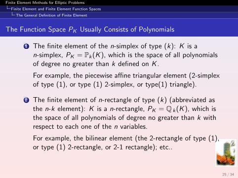
The Function Space PK Usually Consists of Polynomials
1 The finite element of the n-simplex of type (k): K is an-simplex, PK = Pk(K ), which is the space of all polynomialsof degree no greater than k defined on K .
For example, the piecewise affine triangular element (2-simplexof type (1), or type (1) 2-simplex, or type(1) triangle).
2 The finite element of n-rectangle of type (k) (abbreviated asthe n-k element): K is a n-rectangle, PK = Q k(K ), which isthe space of all polynomials of degree no greater than k withrespect to each one of the n variables.
For example, the bilinear element (the 2-rectangle of type (1),or type (1) 2-rectangle, or 2-1 rectangle); etc..
25 / 34
Finite Element Methods for Elliptic Problems
Finite Element and Finite Element Function Spaces
The General Definition of Finite Element
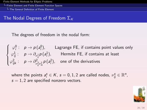
The Nodal Degrees of Freedom ΣK
The degrees of freedom in the nodal form:
ϕ0i : p → p (a0
i ), Lagrange FE, if contains point values only
ϕ1ij : p → ∂ν1
ijp (a1
i ), Hermite FE, if contains at least
ϕ2ijk : p → ∂2
ν2ijν
2ik
p (a2i ), one of the derivatives
where the points asi ∈ K , s = 0, 1, 2 are called nodes, νsij ∈ Rn,s = 1, 2 are specified nonzero vectors.
26 / 34
Finite Element Methods for Elliptic Problems
Finite Element and Finite Element Function Spaces
The General Definition of Finite Element
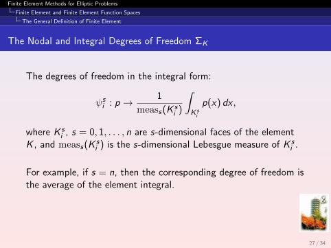
The Nodal and Integral Degrees of Freedom ΣK
The degrees of freedom in the integral form:
ψsi : p → 1
meass(K si )
∫K si
p(x) dx ,
where K si , s = 0, 1, . . . , n are s-dimensional faces of the element
K , and meass(K si ) is the s-dimensional Lebesgue measure of K s
i .
For example, if s = n, then the corresponding degree of freedom isthe average of the element integral.
27 / 34
Finite Element Methods for Elliptic Problems
Finite Element and Finite Element Function Spaces
Finite Element Interpolation
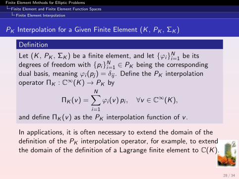
PK Interpolation for a Given Finite Element (K , PK , ΣK )
Definition
Let (K , PK , ΣK ) be a finite element, and let ϕiNi=1 be itsdegrees of freedom with piNi=1 ∈ PK being the correspondingdual basis, meaning ϕi (pj) = δij . Define the PK interpolationoperator ΠK : C∞(K )→ PK by
ΠK (v) =N∑i=1
ϕi (v) pi , ∀v ∈ C∞(K ),
and define ΠK (v) as the PK interpolation function of v .
In applications, it is often necessary to extend the domain of thedefinition of the PK interpolation operator, for example, to extendthe domain of the definition of a Lagrange finite element to C(K ).
28 / 34
Finite Element Methods for Elliptic Problems
Finite Element and Finite Element Function Spaces
Finite Element Interpolation
The PK Interpolation Operator Is Independent of the Choice of Basis
Definition
Let two finite elements (K , PK , ΣK ) and (L, PL, ΣL) satisfy
K = L, PK = PL, and ΠK = ΠL,
where ΠK and ΠL are respectively PK and PL interpolationoperators, then the two finite elements are said to be equivalent.
29 / 34
Finite Element Methods for Elliptic Problems
Finite Element and Finite Element Function Spaces
Finite Element Interpolation
Compatibility Conditions for PK and ΣK on Adjacent Elements
1 Th: a finite element triangulation of Ω; (K ,PK ,ΣK )K∈Th : agiven set of corresponding finite elements.
2 Vh = v :⋃
K∈Th K → R : v |K ∈ PK: FE function space.
3 Compatibility conditions are required to assure Vh satisfies(FEM 3), as well as a subspace of V.
For example, for polyhedron elements and nodal degrees offreedom, if K1
⋂K2 6= ∅, then, we require that a point
asi ∈ K1⋂
K2 is a node of K1, if and only if it is also the same typeof node of K2.
30 / 34
Finite Element Methods for Elliptic Problems
Finite Element and Finite Element Function Spaces
Finite Element Interpolation
Vh Interpolation Operator and Vh Interpolation
Denote Σh =⋃
K∈Th ΣK as the degrees of freedom of the finiteelement function space Vh.
Definition
Define the Vh interpolation operator Πh : C∞(Ω)→ Vh by
Πh(v)|K = ΠK (v |K ), ∀v ∈ C∞(Ω),
and define Πh(v) as the Vh interpolant of v .
In applications, similar as for the PK interpolation operator, thedomain of definition of the Vh interpolation operator is oftenextended to meet certain requirements.
31 / 34
Reference Finite Element (K , P, Σ) and Its Isoparametric Equivalent Family
Definition
Let K , K ∈ Rn, (K , P, Σ) and (K , PK , ΣK ) be two finiteelements. Suppose that there exists a sufficiently smooth invertiblemap FK : K → K , such that
FK (K ) = K ;
pi = pi F−1K , i = 1, . . . ,N;
ϕi (p) = ϕi (p FK ), ∀p ∈ PK , i = 1, . . . ,N,
where ϕiNi=1 and ϕiNi=1 are the basis of the degrees of freedom
spaces Σ and ΣK respectively, piNi=1 and piNi=1 are the
corresponding dual basis of P and PK respectively. Then, the twofinite elements are said to be isoparametrically equivalent. Inparticular, if FK is an affine mapping, the two finite elements aresaid to be affine-equivalent.
Finite Element Methods for Elliptic Problems
Finite Element and Finite Element Function Spaces
Isoparametric and Affine Equivalent Family of Finite Elements
An Isoparametric (Affine) Family of Finite Elements
If all finite elements in a family are isoparametrically (affine-)equivalent to a given reference finite element, then we call thefamily an isoparametric (affine) family.
For example, the finite elements with triangular elements andpiecewise linear function space used in the previous subsection, i.e.finite elements of 2-simplex of type (1), are an affine family.
33 / 34
SK 6µ5, 6, 7
Thank You!