Numerical Methods-Lecture IX: Quadrature (and Markov...

Numerical Methods-Lecture IX:Quadrature (and Markov Chains)

(See Judd Chapter 7, Stokey Lucas Prescott Chapter 11)

Trevor Gallen

Fall, 2015

1 / 40

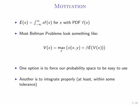
Motivation

I E (x) =∫∞−∞ xf (x) for x with PDF f (x)

I Most Bellman Problems look something like:

V (x) = maxy{φ(x , y) + βE (V (x))}

I One option is to force our probability space to be easy to use

I Another is to integrate properly (at least, within sometolerance)

2 / 40

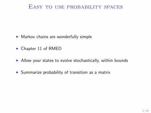
Easy to use probability spaces

I Markov chains are wonderfully simple

I Chapter 11 of RMED

I Allow your states to evolve stochastically, within bounds

I Summarize probability of transition as a matrix

3 / 40

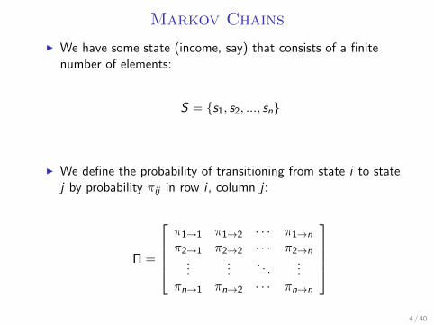
Markov Chains

I We have some state (income, say) that consists of a finitenumber of elements:

S = {s1, s2, ..., sn}

I We define the probability of transitioning from state i to statej by probability πij in row i , column j :

Π =

π1→1 π1→2 · · · π1→n

π2→1 π2→2 · · · π2→n...

.... . .

...πn→1 πn→2 · · · πn→n

4 / 40

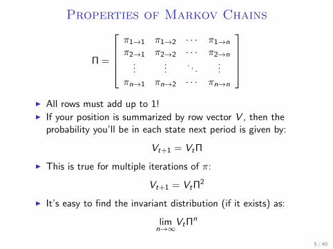
Properties of Markov Chains

Π =

π1→1 π1→2 · · · π1→n

π2→1 π2→2 · · · π2→n...

.... . .

...πn→1 πn→2 · · · πn→n

I All rows must add up to 1!I If your position is summarized by row vector V , then the

probability you’ll be in each state next period is given by:

Vt+1 = VtΠ

I This is true for multiple iterations of π:

Vt+1 = VtΠ2

I It’s easy to find the invariant distribution (if it exists) as:

limn→∞

VtΠn

5 / 40

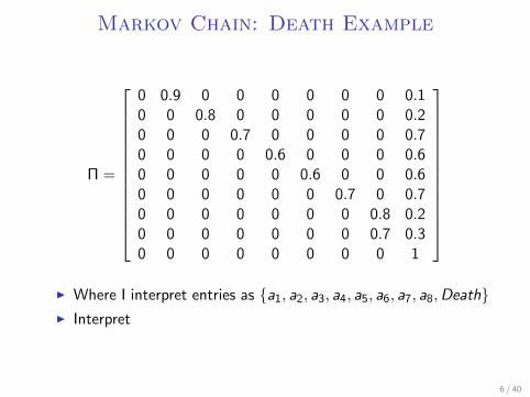
Markov Chain: Death Example

Π =

0 0.9 0 0 0 0 0 0 0.10 0 0.8 0 0 0 0 0 0.20 0 0 0.7 0 0 0 0 0.70 0 0 0 0.6 0 0 0 0.60 0 0 0 0 0.6 0 0 0.60 0 0 0 0 0 0.7 0 0.70 0 0 0 0 0 0 0.8 0.20 0 0 0 0 0 0 0.7 0.30 0 0 0 0 0 0 0 1

I Where I interpret entries as {a1, a2, a3, a4, a5, a6, a7, a8,Death}I Interpret

6 / 40

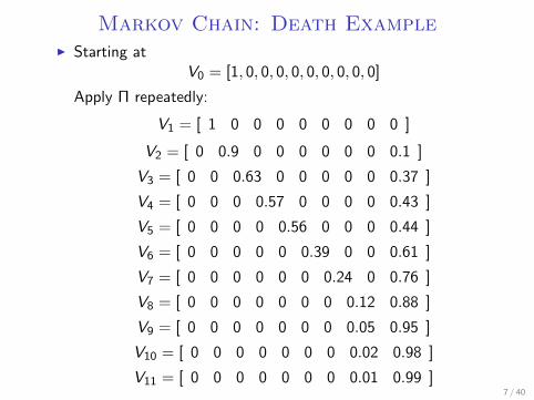
Markov Chain: Death ExampleI Starting at

V0 = [1, 0, 0, 0, 0, 0, 0, 0, 0, 0]

Apply Π repeatedly:

V1 = [ 1 0 0 0 0 0 0 0 0 ]

V2 = [ 0 0.9 0 0 0 0 0 0 0.1 ]

V3 = [ 0 0 0.63 0 0 0 0 0 0.37 ]

V4 = [ 0 0 0 0.57 0 0 0 0 0.43 ]

V5 = [ 0 0 0 0 0.56 0 0 0 0.44 ]

V6 = [ 0 0 0 0 0 0.39 0 0 0.61 ]

V7 = [ 0 0 0 0 0 0 0.24 0 0.76 ]

V8 = [ 0 0 0 0 0 0 0 0.12 0.88 ]

V9 = [ 0 0 0 0 0 0 0 0.05 0.95 ]

V10 = [ 0 0 0 0 0 0 0 0.02 0.98 ]

V11 = [ 0 0 0 0 0 0 0 0.01 0.99 ]7 / 40

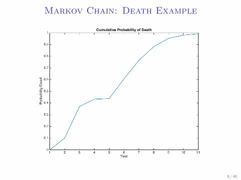
Markov Chain: Death Example

8 / 40

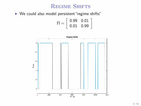
Regime ShiftsI We could also model persistent“regime shifts”

Π =

[0.99 0.010.01 0.99

]

9 / 40

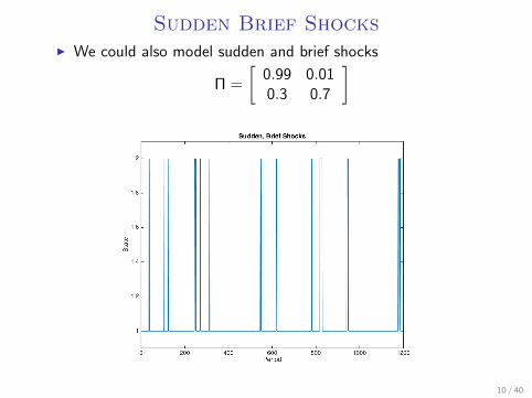
Sudden Brief ShocksI We could also model sudden and brief shocks

Π =

[0.99 0.010.3 0.7

]

10 / 40

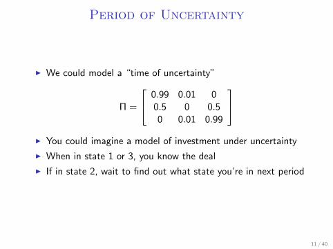
Period of Uncertainty

I We could model a “time of uncertainty”

Π =

0.99 0.01 00.5 0 0.50 0.01 0.99

I You could imagine a model of investment under uncertainty

I When in state 1 or 3, you know the deal

I If in state 2, wait to find out what state you’re in next period

11 / 40

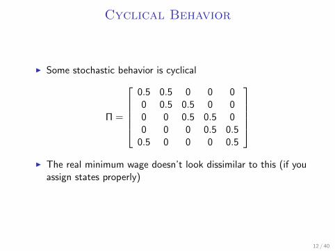
Cyclical Behavior

I Some stochastic behavior is cyclical

Π =

0.5 0.5 0 0 00 0.5 0.5 0 00 0 0.5 0.5 00 0 0 0.5 0.5

0.5 0 0 0 0.5

I The real minimum wage doesn’t look dissimilar to this (if you

assign states properly)

12 / 40

Markov Chains: Summary

I Very flexible, incredibly easy to use, program, simulate

I Easy to estimate using maximum likelihood

I Good for learning problems or any regime shifting problems

I Require discrete states

I Easy to “integrate” and get probabilities

I Don’t leave home without them

13 / 40

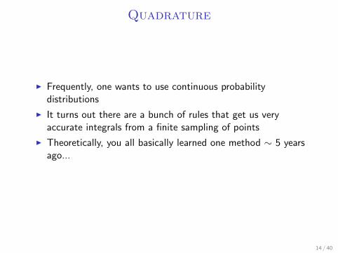
Quadrature

I Frequently, one wants to use continuous probabilitydistributions

I It turns out there are a bunch of rules that get us veryaccurate integrals from a finite sampling of points

I Theoretically, you all basically learned one method ∼ 5 yearsago...

14 / 40

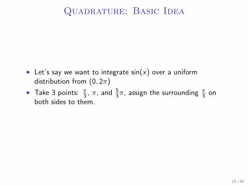
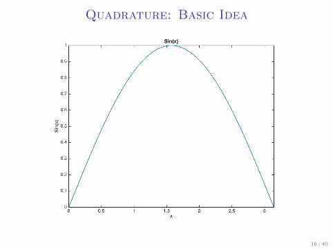
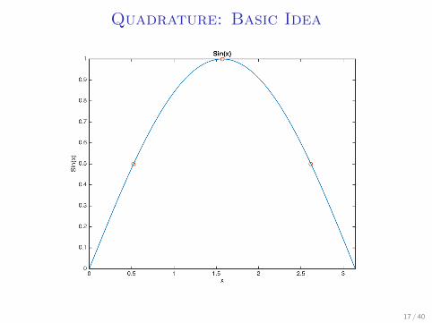
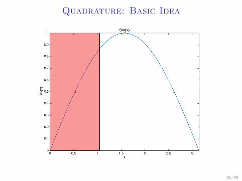
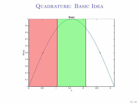
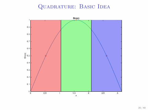
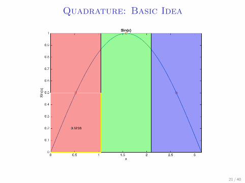
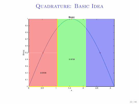
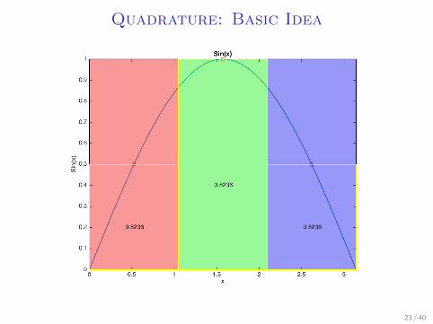
Quadrature: Basic Idea

I Let’s say we want to integrate sin(x) over a uniformdistribution from (0, 2π)

I Take 3 points: π3 , π, and 5

3π, assign the surrounding π3 on

both sides to them.

15 / 40


16 / 40


17 / 40


18 / 40


19 / 40


20 / 40


21 / 40


22 / 40


23 / 40


24 / 40

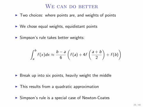
We can do better

I Two choices: where points are, and weights of points

I We chose equal weights, equidistant points

I Simpson’s rule takes better weights:

∫ b

af (x)dx ≈ b − a

6

(f (a) + 4f

(a + b

2

)+ f (b)

)

I Break up into six points, heavily weight the middle

I This results from a quadratic approximation

I Simpson’s rule is a special case of Newton-Coates

25 / 40

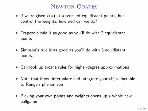
Newton-Coates

I If we’re given f (x) at a series of equidistant points, butcontrol the weights, how well can we do?

I Trapezoid rule is as good as you’ll do with 2 equidistantpoints

I Simpson’s rule is as good as you’ll do with 3 equidistantpoints.

I Can look up arcane rules for higher-degree approximations

I Note that if you interpolate and integrate yourself, vulnerableto Runge’s phenomeon

I Picking your own points and weights opens up a whole newballgame

26 / 40

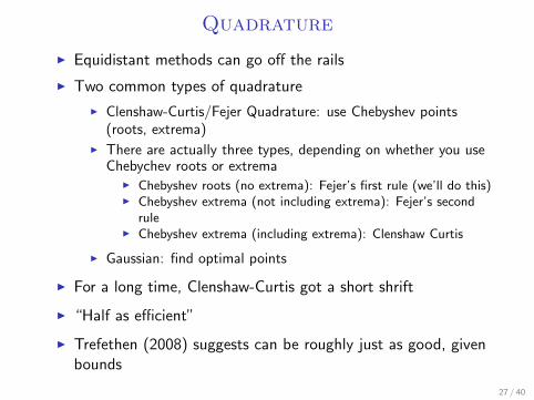
Quadrature

I Equidistant methods can go off the rails

I Two common types of quadrature

I Clenshaw-Curtis/Fejer Quadrature: use Chebyshev points(roots, extrema)

I There are actually three types, depending on whether you useChebychev roots or extrema

I Chebyshev roots (no extrema): Fejer’s first rule (we’ll do this)I Chebyshev extrema (not including extrema): Fejer’s second

ruleI Chebyshev extrema (including extrema): Clenshaw Curtis

I Gaussian: find optimal points

I For a long time, Clenshaw-Curtis got a short shrift

I “Half as efficient”

I Trefethen (2008) suggests can be roughly just as good, givenbounds

27 / 40

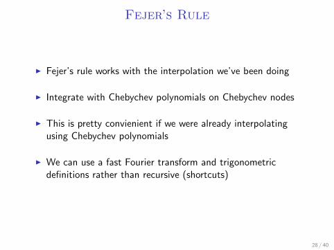
Fejer’s Rule

I Fejer’s rule works with the interpolation we’ve been doing

I Integrate with Chebychev polynomials on Chebychev nodes

I This is pretty convienient if we were already interpolatingusing Chebychev polynomials

I We can use a fast Fourier transform and trigonometricdefinitions rather than recursive (shortcuts)

28 / 40

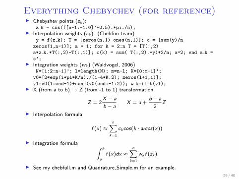
Everything Chebychev (for reference)I Chebyshev points (zk ):

z k = cos(([n-1:-1:0]’+0.5).*pi./n);I Interpolation weights (ck ): (Chebfun team)

y = f(z k); T = [zeros(n,1) ones(n,1)]; c = [sum(y)/n

zeros(1,n-1)]; a = 1; for k = 2:n T = [T(:,2)

a*z k.*T(:,2)-T(:,1)]; c(k) = sum( T(:,2).*y)*2/n; a=2; end a k =

c’;I Integration weights (wk ) (Waldvogel, 2006)

N=[1:2:n-1]’; l=length(N); m=n-l; K=[0:m-1]’;

v0=[2*exp(i*pi*K/n)./(1-4*K.2̂); zeros(l+1,1)];

v1=v0(1:end-1)+conj(v0(end:-1:2)); w k=ifft(v1);I X (from a to b) → Z (from -1 to 1) transformation

Z = 2X − a

b − aX = a+

b − a

2Z

I Interpolation formula

f (x) ≈n∑

k=1

ckcos(k · arcos(x))

I Integration formula ∫ b

af (x)dx ≈

n∑k=1

wk f (zk )

I See my chebfull.m and Quadrature Simple.m for an example.

29 / 40

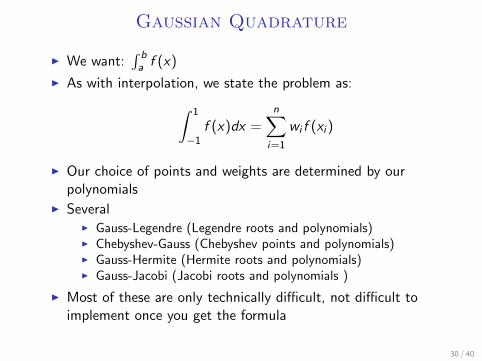
Gaussian Quadrature

I We want:∫ ba f (x)

I As with interpolation, we state the problem as:∫ 1

−1f (x)dx =

n∑i=1

wi f (xi )

I Our choice of points and weights are determined by ourpolynomials

I SeveralI Gauss-Legendre (Legendre roots and polynomials)I Chebyshev-Gauss (Chebyshev points and polynomials)I Gauss-Hermite (Hermite roots and polynomials)I Gauss-Jacobi (Jacobi roots and polynomials )

I Most of these are only technically difficult, not difficult toimplement once you get the formula

30 / 40

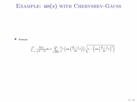
Example: sin(x) with Chebyshev-Gauss

I Formula:

∫ 1

−1

f (x)√1 − x2

dx ≈n∑

i=XXX

π

nf

(cos

(2i − 1

2nπ

))√√√√1 −(cos

(2i − 1

2nπ

)2)

31 / 40

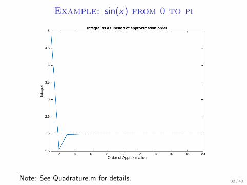
Example: sin(x) from 0 to pi

Note: See Quadrature.m for details. 32 / 40

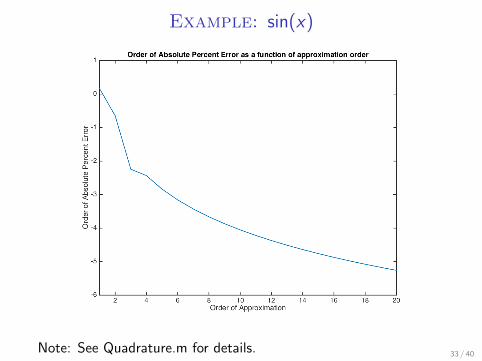
Example: sin(x)

Note: See Quadrature.m for details. 33 / 40

Matlab

I There’s a new guy in town

I Don’t exert thousands of (particularly valuable) man-hourspicking the best polynomials and best points to maximizecomputational efficiency and running horse races

I Nested sets of points to narrow things down is one option

I Or, zoom in on trouble spots, make a more fine approximationthere (Adaptive quadrature)

I Adaptive sparse grid interpolation

I Matlab: Sparse Grid Interpolation Toolbox by Andreas Klimke

34 / 40

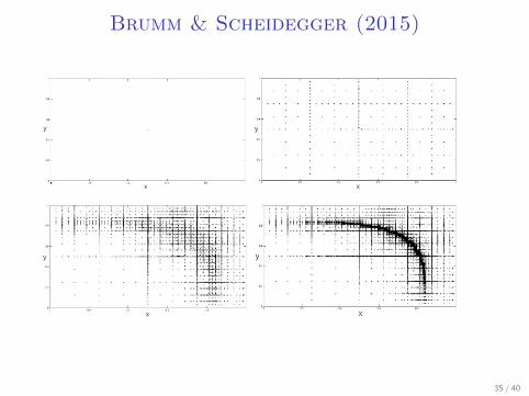
Brumm & Scheidegger (2015)

35 / 40

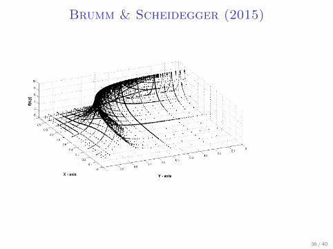
Brumm & Scheidegger (2015)

36 / 40

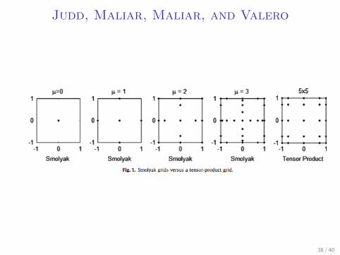
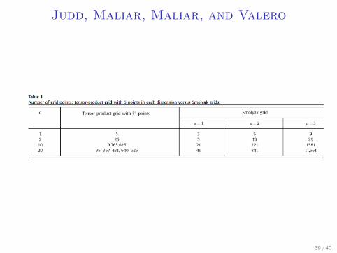
Judd, Maliar, Maliar, and Valero

I Taking every point in grid is inefficient

I Good quick easy toolbox to interpolate and integratefunctions on hypercubes

I Sparse grids can allow you to up your dimensions dramatically

I What does the grid look like?

37 / 40


38 / 40


39 / 40

Later in the Quarter: Monte Carlo Methods

I Analytical integration isn’t always possible

I Numerical quadrature frequently focuses on and has goodproperties in a few dimensions

I Monte Carlo integration has become popular

I We’ll talk about this a little later, but the idea is simple

I “Randomly”∗ walk around the space under the integral andsample points

I Your “sample” will be representative of the “population” butyou can add it up, average it, etc.

40 / 40

Numerical Methods-Lecture IX: Quadrature (and Markov...

Documents

Transcript of Numerical Methods-Lecture IX: Quadrature (and Markov...