Normal Numbers and PseudorandomGenerators∗

David H. Bailey† Jonathan M. Borwein‡

December 4, 2011

Abstract

For an integer b ≥ 2 a real number α is b-normal if, for all m > 0,every m-long string of digits in the base-b expansion of α appears, inthe limit, with frequency b−m. Although almost all reals in [0, 1] areb-normal for every b, it has been rather difficult to exhibit explicitexamples. No results whatsoever are known, one way or the other, forthe class of “natural” mathematical constants, such as π, e,

√2 and

log 2. In this paper, we summarize some previous normality results fora certain class of explicit reals, and then show that a specific memberof this class, while provably 2-normal, is provably not 6-normal. Wethen show that a practical and reasonably effective pseudorandomnumber generator can be defined based on the binary digits of thisconstant, and conclude by sketching out some directions for furtherresearch.

∗Submitted to Heinz Bauschke, ed., Proceedings of the Workshop on Computationaland Analytical Mathematics in Honour of Jonathan Borwein’s 60th Birthday, Springer,2011.†Lawrence Berkeley National Laboratory, Berkeley, CA 94720, DHBailey@lbl.gov.

Supported in part by the Director, Office of Computational and Technology Research,Division of Mathematical, Information, and Computational Sciences of the U.S. Depart-ment of Energy, under contract number DE-AC02-05CH11231.‡Laureate Professor and Director Centre for Computer Assisted Research Mathematics

and its Applications (CARMA), University of Newcastle, Callaghan, NSW 2308, Australia.Distinguished Professor, King Abdulaziz University, Jeddah 80200, Saudi Arabia. Email:jonathan.borwein@newcastle.edu.au.

1

1 Introduction

For an integer b ≥ 2 we say that a real number α is b-normal (or normal baseb) if, for all m > 0, every m-long string of digits in the base-b expansion of αappears, in the limit, with frequency b−m, or, in other words, with exactly thefrequency one would expect if the digits appeared completely “at random.”It follows from basic probability theory that, for any integer b ≥ 2, almostall reals in the interval (0, 1) are b-normal. What’s more, almost all reals inthe unit interval are simultaneously b-normal for all integers b ≥ 2.

Yet identifying even a single explicitly given real number that is b-normalfor some b has proven frustratingly difficult. The first constant proven 10-normal was the Champernowne constant [7], namely 0.12345678910111213 . . .,produced by concatenating the natural numbers in decimal format. This wasextended to base-b normality (for base-b versions of the Champernowne con-stant). In 1946, Copeland and Erdos established that the correspondingconcatenation of primes 0.23571113171923 . . . and also the concatenation ofcomposites 0.46891012141516 . . ., among others, are also 10-normal [8]. Ingeneral they proved:

Theorem 1 ([8]) If a1, a2, · · · is an increasing sequence of integers suchthat for every θ < 1 the number of a’s up to N exceeds N θ provided N issufficiently large, then the infinite decimal

0.a1a2a3 · · ·

is normal with respect to the base β in which these integers are expressed.

This clearly applies to the primes of the form ak + c with a and c relativelyprime in any given base and to the integers which are the sum of two squares(since every prime of the form 4k + 1 is included).

Some related results were established by Schmidt, including the following[15]. Write p ∼ q if there are positive integers r and s such that pr = qs.Then

Theorem 2 If p ∼ q, then any real number that is p-normal is also q-normal. However, if p 6∼ q, then there are uncountably many p-normal realsthat are not q-normal.

In a recent survey, Queffelec [14] described the above result and alsopresented the following, which he ascribed to Korobov:

2

Theorem 3 Numbers of the form∑

k p−2k

q−p2k

, where p and q are relativelyprime, are q-normal.

Nonetheless, we are still completely in the dark as to the b-normality of“natural” constants of mathematics. Borel was the first to conjecture thatall irrational algebraic numbers are b-normal for every integer b ≥ 2. Yetnot a single instance of this conjecture has ever been proven. We do not evenknow for certain whether or not the limiting frequency of zeroes in the binaryexpansion of

√2 is one-half, although numerous large statistical analyses have

failed to show any significant deviation from statistical normals. The samecan be said for π and other basic constants, such as e, log 2 and ζ(3). Clearlyany result (one way or the other) for one of these constants would be amathematical development of the first magnitude.

In the case of an algebraic number of degree d, it is now known thatthe number of ones in the binary expansion through bit position n mustexceed Cn1/d for a positive number C (depending on the constant) and allsufficiently large n [1]. In particular, there must be at least

√n ones in the

first n bits of√

2. But this is clearly a relatively weak result, because, barringan enormous mathematical surprise, the correct limiting frequency of onesin the binary expansion of

√2 is, almost certainly, one-half.

In this paper, we briefly summarize some previously published normalityresults for a certain class of real constants, prove an interesting non-normalityresult, and then demonstrate how these normality results can be parlayedinto producing a practical pseudorandom number generator. This generatorcan be implemented quite easily, is reasonably fast-running, and, in initialtests, seems to produce results of satisfactory “randomness.” In addition, weshow how all of this suggests a future direction to the long sought proof ofnormality for “natural” mathematical constants.

2 Normality of a class of generalized BBP-

type constants

In [3], Richard Crandall and one of the present authors (Bailey) analyzed theclass of constants

αb,c(r) =∞∑k=1

1

ckbck+rk, (1)

3

where the integers b > 1 and c > 1 are co-prime, where r is any real in[0, 1], and where rk is the kth binary digit of r. These constants qualifyas “generalized BBP-type constants,” because the n-th base-b digit can becalculated directly, without needing to compute any of the first n− 1 digits,by a simple and efficient algorithm similar to that first applied to π and log 2in the paper by Bailey, P. Borwein and Plouffe [2].

Bailey and Crandall were able to establish:

Theorem 4 Every real constant of the class (1) is b-normal.

Subsequently, Bailey and Misieurwicz were able to establish this sameresult (at least in a simple demonstrative case) via a much simpler argument,utilizing a “hot spot” lemma proven by ergodic theory techniques [5] (see also[6, pg. 155]).

Fix integers b and c satisfying the above criteria, and let r and s beany reals in [0, 1]. If r 6= s, then αb,c(r) 6= αb,c(s), so that the class Ab,c ={αb,c(r), 0 ≤ r ≤ 1} has uncountably many distinct elements (this was shownby Bailey and Crandall). However, it is not known whether the class Ab,ccontains any constants of mathematical significance, such as π or e.

In this paper we will focus on the constant α2,3(0), which we will denoteas α for short:

α = α2,3(0) =∞∑k=1

1

3k23k (2)

= 0.0418836808315029850712528986245716824260967584654857 . . .10

= 0.0AB8E38F684BDA12F684BF35BA781948B0FCD6E9E06522C3F35B . . .16 .

Although its 2-normality follows from the results in either of the two papersmentioned above ([3] and [5]), this particular constant was first proved 2-normal by Stoneham back in 1973 [16].

3 A non-normality result

It should be emphasized that just because a real constant is b-normal forsome integer b > 1, it does not follow that it is c-normal for any other integerc, except in the case where br = cs for positive integers r and s (see Theorem2). In other words, if a constant is 8-normal, it is clearly 16-normal (sincebase-16 digits can be written as four binary digits and base-8 digits can be

4

written as three binary digits), but nothing can be said a priori about thatconstant’s normality in any base that is not a power of two.

As mentioned above, there are very few normality results, and none isknown for well-known constants of mathematics. But the same can be saidabout specific non-normality results, provided we exclude rationals (which re-peat and thus are not normal) and examples, such as 1.0101000100000001 . . .(i.e., ones appear in position 2m), that are constructed specifically not to benormal but otherwise have relatively little mathematical interest (althoughLiouville’s class of transcendental numbers is an exception). In particular,none of the well-known “natural” constants of mathematics have ever beenproven not to be b-normal for some b. Indeed, such a result, say for π, log 2or√

2, would be even more interesting than a proof of normality for thatconstant.

In that vein, here is an intriguing result regarding the α constant men-tioned above:

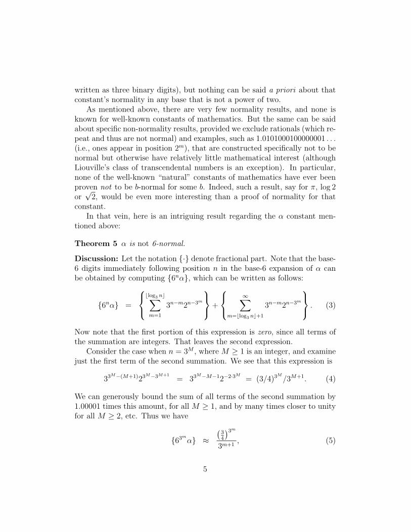
Theorem 5 α is not 6-normal.

Discussion: Let the notation {·} denote fractional part. Note that the base-6 digits immediately following position n in the base-6 expansion of α canbe obtained by computing {6nα}, which can be written as follows:

{6nα} =

blog3 nc∑m=1

3n−m2n−3m

+

∞∑

m=blog3 nc+1

3n−m2n−3m

. (3)

Now note that the first portion of this expression is zero, since all terms ofthe summation are integers. That leaves the second expression.

Consider the case when n = 3M , where M ≥ 1 is an integer, and examinejust the first term of the second summation. We see that this expression is

33M−(M+1)23M−3M+1

= 33M−M−12−2·3M

= (3/4)3M

/3M+1. (4)

We can generously bound the sum of all terms of the second summation by1.00001 times this amount, for all M ≥ 1, and by many times closer to unityfor all M ≥ 2, etc. Thus we have

{63m

α} ≈(

34

)3m

3m+1, (5)

5

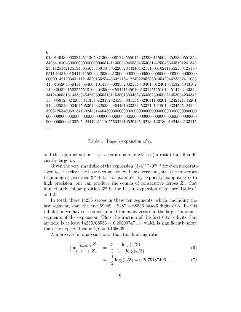
0.0130140430003334251130502130000001243555045432233011500243525320551352343541010430000000000000000514113005404055545530314425043343510124134523511251421251345055035450150535220520443404521515051024115525004251300511244540010441311500324203032130000000000000000000000000000000000000000001421203431112145201352544534211341224022052530105420442355241105541501552043504145554003101453030335320025343404013012401044532543435021420204324150255551010040433000455441145010313314511510144514123443342341240055131333504542353055315115350153345243545025005552145305423434215303501250242054041354512313232453530315345523041150201542421211452015422225343403404505301233255344404431033324453321414150142334545424124320312534005013415024551440430000000000000000000000000000000000000000000000000000000000000000000000000000000000000000000000000000000000000000000000000313350542444431111055534141052014540213412313001424333133115. . .

Table 1: Base-6 expansion of α.

and this approximation is as accurate as one wishes (in ratio) for all suffi-ciently large m.

Given the very small size of the expression (3/4)3m/3m+1 for even moderate-

sized m, it is clear the base-6 expansion will have very long stretches of zeroesbeginning at positions 3m + 1. For example, by explicitly computing α tohigh precision, one can produce the counts of consecutive zeroes Zm thatimmediately follow position 3m in the base-6 expansion of α—see Tables 1and 2.

In total, there 14256 zeroes in these ten segments, which, including thelast segment, span the first 59049 + 9487 = 68536 base-6 digits of α. In thistabulation we have of course ignored the many zeroes in the large “random”segments of the expansion. Thus the fraction of the first 68536 digits thatare zero is at least 14256/68536 = 0.20800747 . . ., which is significantly morethan the expected value 1/6 = 0.166666 . . ..

A more careful analysis shows that this limiting ratio

limm→∞

∑m≥1 Zm

3m + Zm=

3

2· log6(4/3)

1 + log6(4/3)(6)

=1

2log2(4/3) = 0.2075187496 . . . (7)

6

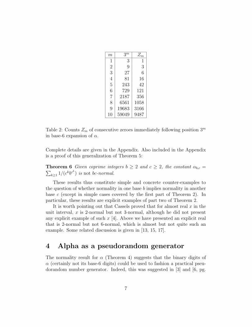
m 3m Zm1 3 12 9 33 27 64 81 165 243 426 729 1217 2187 3568 6561 10589 19683 3166

10 59049 9487

Table 2: Counts Zm of consecutive zeroes immediately following position 3m

in base-6 expansion of α.

Complete details are given in the Appendix. Also included in the Appendixis a proof of this generalization of Theorem 5:

Theorem 6 Given coprime integers b ≥ 2 and c ≥ 2, the constant αb,c =∑k≥1 1/(ckbc

k) is not bc-normal.

These results thus constitute simple and concrete counter-examples tothe question of whether normality in one base b implies normality in anotherbase c (except in simple cases covered by the first part of Theorem 2). Inparticular, these results are explicit examples of part two of Theorem 2.

It is worth pointing out that Cassels proved that for almost real x in theunit interval, x is 2-normal but not 3-normal, although he did not presentany explicit example of such x [4]. Above we have presented an explicit realthat is 2-normal but not 6-normal, which is almost but not quite such anexample. Some related discussion is given in [13, 15, 17].

4 Alpha as a pseudorandom generator

The normality result for α (Theorem 4) suggests that the binary digits ofα (certainly not its base-6 digits) could be used to fashion a practical pseu-dorandom number generator. Indeed, this was suggested in [3] and [6, pg.

7

169–170]. We will show here how this can be done. The result is a genera-tor that is both efficient on single-processor systems and also well-suited forparallel processing: each processor can quickly and independently calculatethe starting seed for its section of the resulting global sequence, which globalsequence is the same as the sequence produced on a single-processor system(subject to some reasonable conditions). However, it is acknowledged thatbefore such a generator is used in a “practical” application, it must be sub-jected to significant checking and testing. It should also be noted that justbecause a number is normal does not guarantee its suitability for pseudo-random generation (e.g., the convergence of the limiting frequencies mightbe very slow), although this particular scheme does appear to be reasonablywell-behaved.

4.1 Background

Define xn to be the binary expansion of α starting with position n+ 1. Notethat xn = {2nα}, where {·} means the fractional part of the argument. Firstconsider the case n = 3m for some integer m. In this case one can write

x3m = {23m

α} =

{m∑k=1

23m−3k

3k

}+

∞∑k=m+1

23m−3k

3k. (8)

Observe that the “tail” term (i.e., the second term) in this expression isexceedingly small once m is even moderately large—for example, when m =10, this term is only about 10−35551. This term will hereafter be abbreviatedas εm. By expanding the first term, one obtains

x3m =(3m−123m−3 + 3m−223m−32

+ · · ·+ 3 · 23m−3m−1+ 1) mod 3m

3m

+εm (9)

The numerator is taken modulo 3m, since only the remainder when dividedby 3m is of interest when finding the fractional part. By Euler’s totienttheorem, the next-to-last term in the numerator, when reduced modulo 3m,is three. Similarly, it can be seen that every other term in the numerator,when reduced modulo 3m, is equivalent to itself without the power-of-two

8

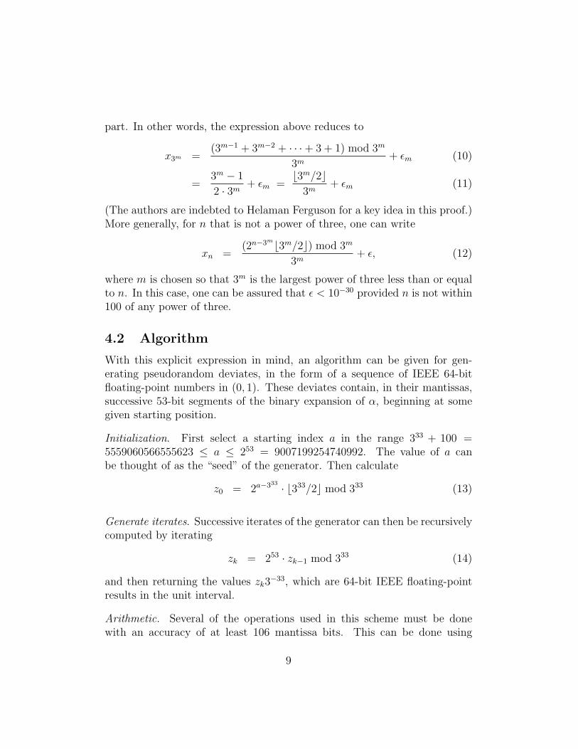
part. In other words, the expression above reduces to

x3m =(3m−1 + 3m−2 + · · ·+ 3 + 1) mod 3m

3m+ εm (10)

=3m − 1

2 · 3m+ εm =

b3m/2c3m

+ εm (11)

(The authors are indebted to Helaman Ferguson for a key idea in this proof.)More generally, for n that is not a power of three, one can write

xn =(2n−3mb3m/2c) mod 3m

3m+ ε, (12)

where m is chosen so that 3m is the largest power of three less than or equalto n. In this case, one can be assured that ε < 10−30 provided n is not within100 of any power of three.

4.2 Algorithm

With this explicit expression in mind, an algorithm can be given for gen-erating pseudorandom deviates, in the form of a sequence of IEEE 64-bitfloating-point numbers in (0, 1). These deviates contain, in their mantissas,successive 53-bit segments of the binary expansion of α, beginning at somegiven starting position.

Initialization. First select a starting index a in the range 333 + 100 =5559060566555623 ≤ a ≤ 253 = 9007199254740992. The value of a canbe thought of as the “seed” of the generator. Then calculate

z0 = 2a−333 · b333/2c mod 333 (13)

Generate iterates. Successive iterates of the generator can then be recursivelycomputed by iterating

zk = 253 · zk−1 mod 333 (14)

and then returning the values zk3−33, which are 64-bit IEEE floating-point

results in the unit interval.

Arithmetic. Several of the operations used in this scheme must be donewith an accuracy of at least 106 mantissa bits. This can be done using

9

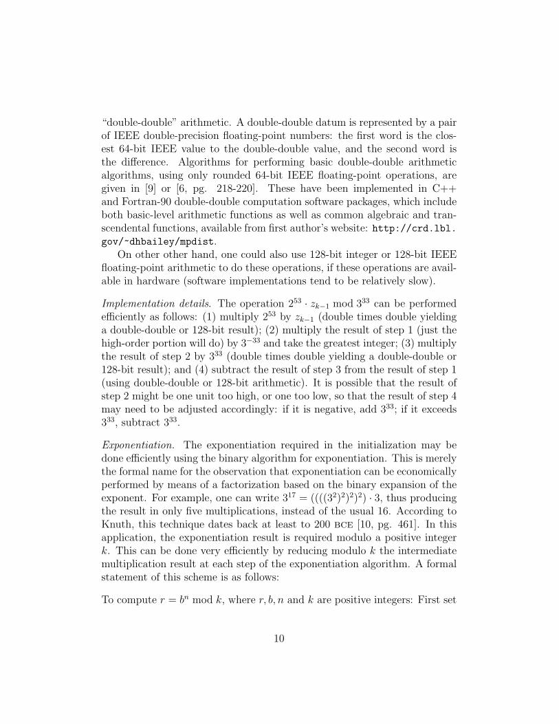
“double-double” arithmetic. A double-double datum is represented by a pairof IEEE double-precision floating-point numbers: the first word is the clos-est 64-bit IEEE value to the double-double value, and the second word isthe difference. Algorithms for performing basic double-double arithmeticalgorithms, using only rounded 64-bit IEEE floating-point operations, aregiven in [9] or [6, pg. 218-220]. These have been implemented in C++and Fortran-90 double-double computation software packages, which includeboth basic-level arithmetic functions as well as common algebraic and tran-scendental functions, available from first author’s website: http://crd.lbl.gov/~dhbailey/mpdist.

On other other hand, one could also use 128-bit integer or 128-bit IEEEfloating-point arithmetic to do these operations, if these operations are avail-able in hardware (software implementations tend to be relatively slow).

Implementation details. The operation 253 · zk−1 mod 333 can be performedefficiently as follows: (1) multiply 253 by zk−1 (double times double yieldinga double-double or 128-bit result); (2) multiply the result of step 1 (just thehigh-order portion will do) by 3−33 and take the greatest integer; (3) multiplythe result of step 2 by 333 (double times double yielding a double-double or128-bit result); and (4) subtract the result of step 3 from the result of step 1(using double-double or 128-bit arithmetic). It is possible that the result ofstep 2 might be one unit too high, or one too low, so that the result of step 4may need to be adjusted accordingly: if it is negative, add 333; if it exceeds333, subtract 333.

Exponentiation. The exponentiation required in the initialization may bedone efficiently using the binary algorithm for exponentiation. This is merelythe formal name for the observation that exponentiation can be economicallyperformed by means of a factorization based on the binary expansion of theexponent. For example, one can write 317 = ((((32)2)2)2) · 3, thus producingthe result in only five multiplications, instead of the usual 16. According toKnuth, this technique dates back at least to 200 bce [10, pg. 461]. In thisapplication, the exponentiation result is required modulo a positive integerk. This can be done very efficiently by reducing modulo k the intermediatemultiplication result at each step of the exponentiation algorithm. A formalstatement of this scheme is as follows:

To compute r = bn mod k, where r, b, n and k are positive integers: First set

10

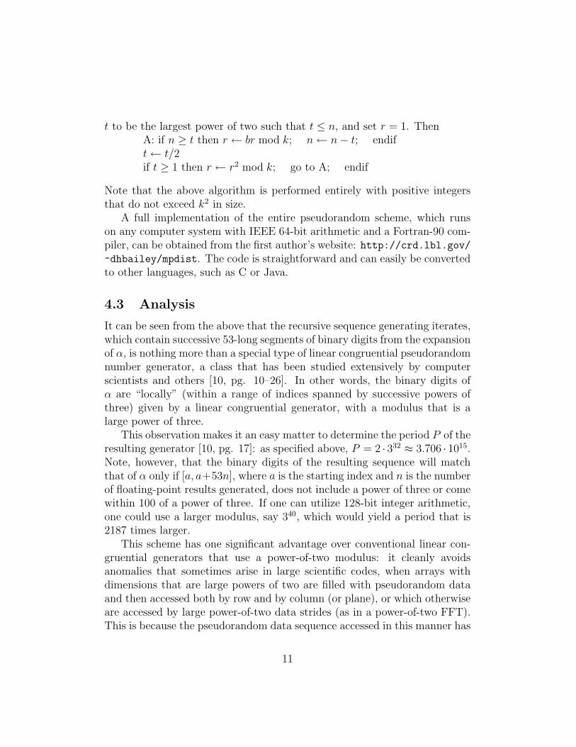
t to be the largest power of two such that t ≤ n, and set r = 1. ThenA: if n ≥ t then r ← br mod k; n← n− t; endift← t/2if t ≥ 1 then r ← r2 mod k; go to A; endif

Note that the above algorithm is performed entirely with positive integersthat do not exceed k2 in size.

A full implementation of the entire pseudorandom scheme, which runson any computer system with IEEE 64-bit arithmetic and a Fortran-90 com-piler, can be obtained from the first author’s website: http://crd.lbl.gov/

~dhbailey/mpdist. The code is straightforward and can easily be convertedto other languages, such as C or Java.

4.3 Analysis

It can be seen from the above that the recursive sequence generating iterates,which contain successive 53-long segments of binary digits from the expansionof α, is nothing more than a special type of linear congruential pseudorandomnumber generator, a class that has been studied extensively by computerscientists and others [10, pg. 10–26]. In other words, the binary digits ofα are “locally” (within a range of indices spanned by successive powers ofthree) given by a linear congruential generator, with a modulus that is alarge power of three.

This observation makes it an easy matter to determine the period P of theresulting generator [10, pg. 17]: as specified above, P = 2 · 332 ≈ 3.706 · 1015.Note, however, that the binary digits of the resulting sequence will matchthat of α only if [a, a+53n], where a is the starting index and n is the numberof floating-point results generated, does not include a power of three or comewithin 100 of a power of three. If one can utilize 128-bit integer arithmetic,one could use a larger modulus, say 340, which would yield a period that is2187 times larger.

This scheme has one significant advantage over conventional linear con-gruential generators that use a power-of-two modulus: it cleanly avoidsanomalies that sometimes arise in large scientific codes, when arrays withdimensions that are large powers of two are filled with pseudorandom dataand then accessed both by row and by column (or plane), or which otherwiseare accessed by large power-of-two data strides (as in a power-of-two FFT).This is because the pseudorandom data sequence accessed in this manner has

11

a reduced period, and thus may be not as “random” as desired. The usage ofa modulus that is a large power of three is immune to these problems. Theauthors are not aware of any major scientific calculation that involves dataaccess strides that are large powers of three.

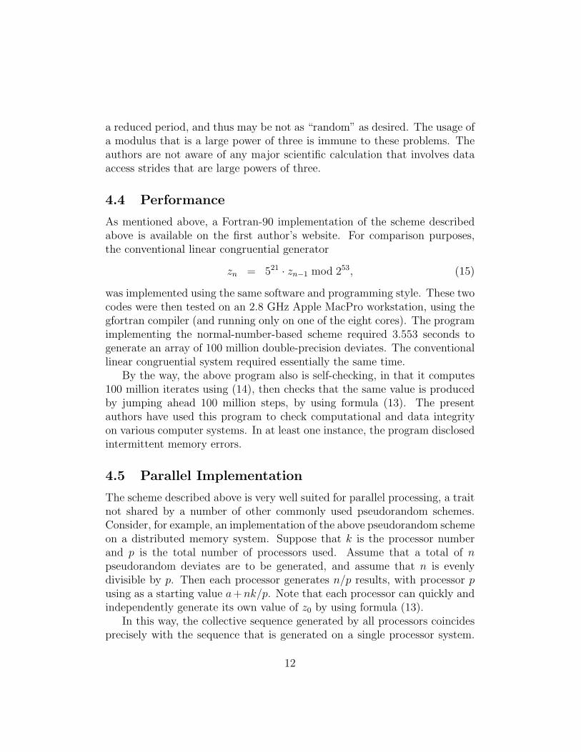
4.4 Performance

As mentioned above, a Fortran-90 implementation of the scheme describedabove is available on the first author’s website. For comparison purposes,the conventional linear congruential generator

zn = 521 · zn−1 mod 253, (15)

was implemented using the same software and programming style. These twocodes were then tested on an 2.8 GHz Apple MacPro workstation, using thegfortran compiler (and running only on one of the eight cores). The programimplementing the normal-number-based scheme required 3.553 seconds togenerate an array of 100 million double-precision deviates. The conventionallinear congruential system required essentially the same time.

By the way, the above program also is self-checking, in that it computes100 million iterates using (14), then checks that the same value is producedby jumping ahead 100 million steps, by using formula (13). The presentauthors have used this program to check computational and data integrityon various computer systems. In at least one instance, the program disclosedintermittent memory errors.

4.5 Parallel Implementation

The scheme described above is very well suited for parallel processing, a traitnot shared by a number of other commonly used pseudorandom schemes.Consider, for example, an implementation of the above pseudorandom schemeon a distributed memory system. Suppose that k is the processor numberand p is the total number of processors used. Assume that a total of npseudorandom deviates are to be generated, and assume that n is evenlydivisible by p. Then each processor generates n/p results, with processor pusing as a starting value a+nk/p. Note that each processor can quickly andindependently generate its own value of z0 by using formula (13).

In this way, the collective sequence generated by all processors coincidesprecisely with the sequence that is generated on a single processor system.

12

This feature is crucially important in parallel processing, permitting onecan verify that a parallel program produces the same answers (to withinreasonable numerical round-off error) as the single-processor version. It isalso important, for the same reason, to permit one to compare results, say,between a run on 64 CPUs of a given system with one on 128 CPUs.

This scheme has been used to generate data for the fast Fourier transform(FFT) benchmark that is part of the benchmark suite for the High Produc-tivity Computing Systems (HPCS) program, funded by the U.S. DefenseAdvanced Research Projects Agency (DARPA) and the U.S. Department ofEnergy.

4.6 Variations

Some initial tests, conducted by Nelson Beebe of the University of Utah,found that if by chance one iterate is rather small, it will include as itstrailing bits a few of the leading bits of the next result (this is a naturalconsequence of the construction). While the authors are not aware of anyapplication for which this feature would have significant impact, it can bevirtually eliminated by advancing the sequence by more than 53 bits—sayby 64 bits—from iterate to iterate.

This can be done by simply altering formula (14) above to read:

zk = 264 · zk−1 mod 333. (16)

This can be implemented as is, if one is using 128-bit integer or 128-bit IEEEfloating-point arithmetic, but does not work correctly if one is using double-double arithmetic, because the product 264 · zk−1 could exceed 2106, which isthe maximum size of an integer that can be represented exactly as a double-double operand. When using double-double arithmetic, one can computeeach iterate using the following:

zk = 211 · (253 · zk−1 mod 333) mod 333. (17)

Tests by the present authors, advancing 64 bits per result, showed no signif-icant correlation to the leading bits of the next iterate. And, of course, theadditional “skip” here could be more than 11; it could be any value up to 53.

Finally, there is no reason that other constants from this class could notalso be used in a similar way. For example, a very similar generator could be

13

constructed based on α2,5. One could also construct pseudorandom genera-tors based on constants that are 3-normal or 5-normal, although one wouldlose the property that successive digits are precisely retained in consecutivecomputer words (which are based on binary arithmetic). The specific choiceof multiplier and modulus can be made based on application requirementsand the type of high-precision arithmetic that is available (e.g., double-doubleor 128-bit integer).

However, as we noted above, it is important to recognize that any pro-posed pseudorandom number generator, including this one, must be sub-jected to lengthy and rigorous testing [10, 11, 12]. Along this line, as notedabove, generators of the general linear congruential family have problems,and it is not yet certain whether some variation or combination of genera-tors in this class can be fashioned into a robust, reliable scheme that is bothefficient and practical. But we do believe that these schemes are worthy offurther study.

5 Conclusion and directions for further work

In this paper, we have shown how the constant α =∑

n≥1 1/(3n23n), which

is provably 2-normal, is not 6-normal, as well as some generalizations. Theseresults thus constitute simple and concrete counter-examples to the ques-tion of whether normality in one base b implies normality in another basec (except in simple cases covered by the first part of Theorem 2). In par-ticular, these results are explicit examples of the second part of Theorem 2.We have also shown how a practical pseudorandom number generator canbe constructed based on the binary digits of α, where each generated wordconsists of successive sections of its binary expansion.

Perhaps the most significant implication of the algorithm we have pre-sented is not for its practical utility, but instead for the insight it providesto the fundamental question of normality. In particular, the pseudorandomnumber construction implies that the digit expansions of one particular classof provably normal numbers consist of successive segments of exponentiallygrowing length, and within each segment the digits are given by a specifictype of linear congruential generator, with a period that also grows exponen-tially. From this perspective, the 2-normality of α is entirely plausible.

Now consider what this implies, say, for the normality of a constant such

14

as log 2. First recall the classical formula

log 2 =∞∑n=1

1

n2n. (18)

Thus, following the well-known BBP approach (see [2] or [6, Chap. 4]), wecan write

{2d log 2} =

{d∑

n=1

2d−n mod n

n

}+

{∞∑

n=d+1

2d−n

n

}. (19)

This leads immediately to the BBP algorithm for computing the binary dig-its of log 2 beginning after position d, since each term of the first summationcan be computed very rapidly by means of the binary algorithm for expo-nentiation, and the second summation quickly converges.

But we can also view (19) for its insight on normality. Note that thebinary expansion of log 2 following position d can be seen as a sum of nor-malized linear congruential pseudorandom number generators, with periods(at least in some terms) that grow steadily with n (since the period of alinear congruential generator depends on the factorization of the modulus).But with increasing n, at least some terms will have prime moduli, resultingin relatively long periods. In fact, some will be primitive primes modulo two,which give the maximal period (n− 1)/2. Note that the sum of normalizedlinear congruential generators can be rewritten as a single linear congruentialgenerator. Thus it is plausible that the period of the sum of generators in thefirst portion of (19) increases without bound, resulting in a highly “random”expansion (although all of this needs to be worked out in detail).

We have attempted to develop these notions further, but so far we havenot made a great deal of progress. But, at the least, this approach may beeffective for constants such as

β =∞∑

n∈W

1

n2n, (20)

where W is the set of primitive primes modulo two, which as mentioned abovegive rise to a maximal periods when used as a linear congruential modulus.Only time will tell.

15

6 Appendix

Proof of Theorem 5: α2,3 is not 6-normal.

Let Qm be the base-6 expansion of α2,3 immediately following position3m (i.e., after the “decimal” point has been shifted to the right 3m digits).We can write

Qm = 63m

α2,3 mod 1

=

(m∑k=1

33m−k23m−3k

)mod 1 +

∞∑k=m+1

33m−k23m−3k

. (21)

The first portion of this expression is zero, since all terms in the summationare integers. The small second portion is very accurately approximated bythe first term of the series, namely (3/4)3m

/3m+1. In fact, for all m ≥ 1,

(3/4)3m

3m+1< Qm <

(3/4)3m

3m+1(1 + 2 · 10−6). (22)

Let Zm = blog6 1/Qmc be the number of zeroes in the base-6 expansionof α that immediately follow position 3m. Then for all m ≥ 1, (22) can berewritten

3m log6

(4

3

)+ (m+ 1) log6 3− 2

< Zm < 3m log6

(4

3

)+ (m+ 1) log6 3. (23)

Now let Fm be the fraction of zeroes in the base-6 expansion of α up toposition 3m +Zm (i.e., up to the end of the block of zeroes that immediatelyfollows position 3m). Clearly

Fm >

∑mk=1 Zk

3m + Zm, (24)

since the numerator only counts zeroes in the long stretches. The summationin the numerator satisfies, for all sufficiently large m,

m∑k=1

Zk >3

2

(3m − 1

3

)log6

(4

3

)+m(m+ 3)

2log6 3− 2m

>3

2· 3m log6

(4

3

)− 1

2log6

(4

3

)− 2m. (25)

16

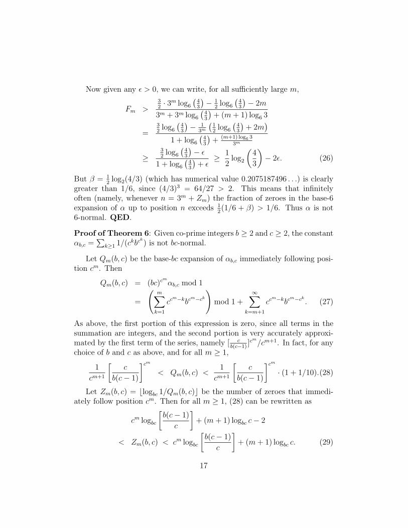
Now given any ε > 0, we can write, for all sufficiently large m,

Fm >32· 3m log6

(43

)− 1

2log6

(43

)− 2m

3m + 3m log6

(43

)+ (m+ 1) log6 3

=32

log6

(43

)− 1

3m

(12

log6

(43

)+ 2m

)1 + log6

(43

)+ (m+1) log6 3

3m

≥32

log6

(43

)− ε

1 + log6

(43

)+ ε

≥ 1

2log2

(4

3

)− 2ε. (26)

But β = 12

log2(4/3) (which has numerical value 0.2075187496 . . .) is clearlygreater than 1/6, since (4/3)3 = 64/27 > 2. This means that infinitelyoften (namely, whenever n = 3m + Zm) the fraction of zeroes in the base-6expansion of α up to position n exceeds 1

2(1/6 + β) > 1/6. Thus α is not

6-normal. QED.

Proof of Theorem 6: Given co-prime integers b ≥ 2 and c ≥ 2, the constantαb,c =

∑k≥1 1/(ckbc

k) is not bc-normal.

Let Qm(b, c) be the base-bc expansion of αb,c immediately following posi-tion cm. Then

Qm(b, c) = (bc)cm

αb,c mod 1

=

(m∑k=1

ccm−kbc

m−ck)

mod 1 +∞∑

k=m+1

ccm−kbc

m−ck . (27)

As above, the first portion of this expression is zero, since all terms in thesummation are integers, and the second portion is very accurately approxi-mated by the first term of the series, namely [ c

b(c−1)]c

m/cm+1. In fact, for any

choice of b and c as above, and for all m ≥ 1,

1

cm+1

[c

b(c− 1)

]cm< Qm(b, c) <

1

cm+1

[c

b(c− 1)

]cm· (1 + 1/10).(28)

Let Zm(b, c) = blogbc 1/Qm(b, c)c be the number of zeroes that immedi-ately follow position cm. Then for all m ≥ 1, (28) can be rewritten as

cm logbc

[b(c− 1)

c

]+ (m+ 1) logbc c− 2

< Zm(b, c) < cm logbc

[b(c− 1)

c

]+ (m+ 1) logbc c. (29)

17

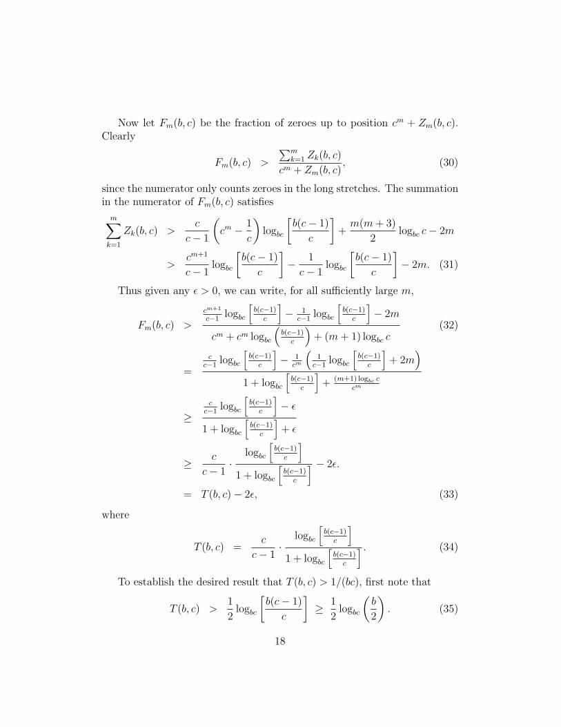
Now let Fm(b, c) be the fraction of zeroes up to position cm + Zm(b, c).Clearly

Fm(b, c) >

∑mk=1 Zk(b, c)

cm + Zm(b, c), (30)

since the numerator only counts zeroes in the long stretches. The summationin the numerator of Fm(b, c) satisfies

m∑k=1

Zk(b, c) >c

c− 1

(cm − 1

c

)logbc

[b(c− 1)

c

]+m(m+ 3)

2logbc c− 2m

>cm+1

c− 1logbc

[b(c− 1)

c

]− 1

c− 1logbc

[b(c− 1)

c

]− 2m. (31)

Thus given any ε > 0, we can write, for all sufficiently large m,

Fm(b, c) >

cm+1

c−1logbc

[b(c−1)c

]− 1

c−1logbc

[b(c−1)c

]− 2m

cm + cm logbc

(b(c−1)c

)+ (m+ 1) logbc c

(32)

=

cc−1

logbc

[b(c−1)c

]− 1

cm

(1c−1

logbc

[b(c−1)c

]+ 2m

)1 + logbc

[b(c−1)c

]+ (m+1) logbc c

cm

≥cc−1

logbc

[b(c−1)c

]− ε

1 + logbc

[b(c−1)c

]+ ε

≥ c

c− 1·

logbc

[b(c−1)c

]1 + logbc

[b(c−1)c

] − 2ε.

= T (b, c)− 2ε, (33)

where

T (b, c) =c

c− 1·

logbc

[b(c−1)c

]1 + logbc

[b(c−1)c

] . (34)

To establish the desired result that T (b, c) > 1/(bc), first note that

T (b, c) >1

2logbc

[b(c− 1)

c

]≥ 1

2logbc

(b

2

). (35)

18

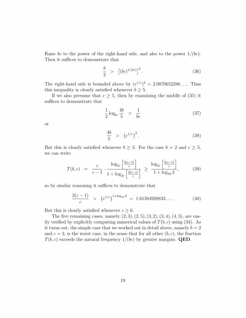
Raise bc to the power of the right-hand side, and also to the power 1/(bc).Then it suffices to demonstrate that

b

2>

[(bc)1/(bc)

]2. (36)

The right-hand side is bounded above by (e1/e)2 = 2.0870652286 . . .. Thusthis inequality is clearly satisfied whenever b ≥ 5.

If we also presume that c ≥ 5, then by examining the middle of (35) itsuffices to demonstrate that

1

2logbc

4b

5>

1

bc(37)

or

4b

5>

(e1/e)2. (38)

But this is clearly satisfied whenever b ≥ 3. For the case b = 2 and c ≥ 5,we can write

T (b, c) =c

c− 1·

log2c

[2(c−1)c

]1 + log2c

[2(c−1)c

] ≥ log2c

[2(c−1)c

]1 + log10 2

, (39)

so by similar reasoning it suffices to demonstrate that

2(c− 1)

c>

(e1/e)1+log10 2

= 1.61384928833 . . . . (40)

But this is clearly satisfied whenever c ≥ 6.The five remaining cases, namely (2, 3), (2, 5), (3, 2), (3, 4), (4, 3), are eas-

ily verified by explicitly computing numerical values of T (b, c) using (34). Asit turns out, the simple case that we worked out in detail above, namely b = 2and c = 3, is the worst case, in the sense that for all other (b, c), the fractionT (b, c) exceeds the natural frequency 1/(bc) by greater margins. QED.

19

References

[1] David H. Bailey, Jonathan M. Borwein, Richard E. Crandall and CarlPomerance, “On the binary expansions of algebraic numbers,” Journalof Number Theory Bordeaux, vol. 16 (2004), pg. 487–518.

[2] David H. Bailey, Peter B. Borwein and Simon Plouffe, “On the rapidcomputation of various polylogarithmic constants,” Mathematics ofComputation, vol. 66, no. 218 (Apr 1997), pg. 903–913.

[3] David H. Bailey and Richard E. Crandall, “Random generators andnormal numbers,” Experimental Mathematics, vol. 11 (2002), no. 4, pg.527–546.

[4] J. W. S. Cassels, “On a problem of Steinhaus about normal numbers,”Colloquium Mathematicum, voo. 7 (1959), pg. 95–101.

[5] David H. Bailey and Michal Misiurewicz, “A strong hot spot theorem,”Proceedings of the American Mathematical Society, vol. 134 (2006), no.9, pg. 2495–2501.

[6] Jonathan M. Borwein and David H. Bailey, Mathematics by Experiment:Plausible Reasoning in the 21st Century, AK Peters, Natick, MA, anded., 2008.

[7] D. G. Champernowne, “The construction of decimals normal in the scaleof ten,” Journal of the London Mathematical Society, vol. 8 (1933), pg.254–260.

[8] A. H. Copeland and P. Erdos, “Note on normal numbers,” Bulletin ofthe American Mathematical Society, vol. 52 (1946), pg. 857–860.

[9] Yozo Hida, Xiaoye S. Li and David H. Bailey, “Algorithms for quad-double precision floating point arithmetic,” 15th IEEE Symposium onComputer Arithmetic, IEEE Computer Society, 2001, pg. 155–162.

[10] Donald E. Knuth, The Art of Computer Programming, vol. 2, Addison-Wesley, Boston, 1998.

[11] P. L’Ecuyer, “Random number generation,” in Handbook of Computa-tional Statistics, J. E. Gentle, W. Haerdle and Y. Mori, ed., Springer-Verlag, Berlin, 2004, Chap. II.2.

20

[12] P. L’Ecuyer and R. Simard, “TestU01: A C Library for empirical test-ing of random number generators,” ACM Transactions on MathematicalSoftware, vol. 33 (Aug. 2007).

[13] A. D. Pollington, “The Hausdorff dimension of a set of normal numbers,”Pacific Journal of Mathematics, vol. 95 (1981), pg. 193–204.

[14] Martine Queffelec, “Old and new results on normality,” Lecture Notes –Monograph Series, vol. 48, Dynamics and Stochastics, 2006, Institute ofMathematical Statistics, pg. 225–236.

[15] W. Schmidt, “On normal numbers,” Pacific Journal of Mathematics,vol. 10 (1960), pg. 661–672.

[16] R. Stoneham, “On absolute (j, ε)-normality in the rational fractions withapplications to normal numbers,” Acta Arithmetica, vol. 22 (1973), 277–286.

[17] H. Weyl, “Uber die Gleichverteilung von Zahlen mod. Eins,” Mathema-tische Annalen, vol. 77 (1916), pg. 313–352.

21