Nonlinear Models - csd.uwo.cadlizotte/teaching/cs4414_F18/Lectures/8_Nonlinear... · Nonlinear...
58
Nonlinear Models Dan Lizotte 2018-10-18 Nonlinearly separable data • A linear boundary might be too simple to capture the class structure. • One way of getting a nonlinear decision boundary in the input space is to find a linear decision boundary in an expanded space (similar to polynomial regression.) • Thus, x i is replaced by ϕ(x i ), where ϕ is called a feature mapping Separability by adding features -2 -1 0 1 2 -1 -0.5 0 0.5 1 x 1 -2 -1 0 1 2 0 0.5 1 1.5 2 2.5 x 1 x 2 = x 1 2 1
Transcript of Nonlinear Models - csd.uwo.cadlizotte/teaching/cs4414_F18/Lectures/8_Nonlinear... · Nonlinear...
Nonlinear ModelsDan Lizotte2018-10-18
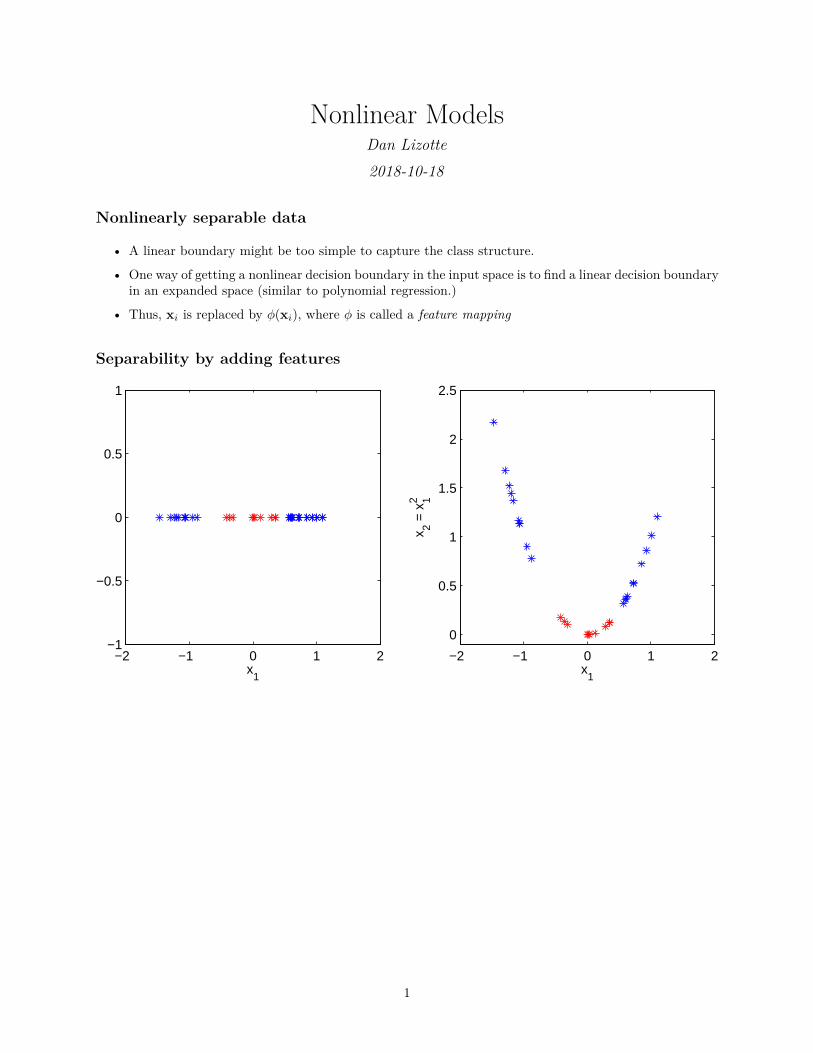
Nonlinearly separable data
• A linear boundary might be too simple to capture the class structure.
• One way of getting a nonlinear decision boundary in the input space is to find a linear decision boundaryin an expanded space (similar to polynomial regression.)
• Thus, xi is replaced by ϕ(xi), where ϕ is called a feature mapping
Separability by adding features
−2 −1 0 1 2−1
−0.5
0
0.5
1
x1
−2 −1 0 1 2
0
0.5
1
1.5
2
2.5
x1
x 2 = x
12
1
Separability by adding features
−2 −1 0 1 2−1
−0.5
0
0.5
1
x
(w0+w(1) x+w(2) x2)
−2 −1 0 1 2
0
0.5
1
1.5
2
2.5
x1
x 2 = x
12
Separability by adding features
−2 −1 0 1 2−1
−0.5
0
0.5
1
x
(w0+w(1) x+w(2) x2)
−2 −1 0 1 2
0
0.5
1
1.5
2
2.5
x
x 2 = x
12
b(1)+b(2) x
more flexible decision boundary ≈ enriched feature space
Margin optimization in feature space
• Replacing xi with ϕ(xi), the dual form becomes:
2
max∑n
i=1 αi − 12∑n
i,j=1 yiyjαiαj(ϕ(xi) · ϕ(xj))w.r.t. αi
s.t. 0 ≤ αi ≤ C and∑n
i=1 αiyi = 0
• Classification of an input x is given by:
hw,w0(x) = sign(
n∑i=1
αiyi(ϕ(xi) · ϕ(x)) + w0
)
• Note that in the dual form, to do both SVM training and prediction, we only ever need to computedot-products of feature vectors.
Kernel functions
• Whenever a learning algorithm (such as SVMs) can be written in terms of dot-products, it can begeneralized to kernels.
• A kernel is any function K : Rn × Rn 7→ R which corresponds to a dot product for some featuremapping ϕ:
K(x1, x2) = ϕ(x1) · ϕ(x2) for some ϕ.
• Conversely, by choosing feature mapping ϕ, we implicitly choose a kernel function
• Recall that ϕ(x1) · ϕ(x2) ∝ cos∠(ϕ(x1), ϕ(x2)) where ∠ denotes the angle between the vectors, so akernel function can be thought of as a notion of similarity.
Example: Quadratic kernel
• Let K(x, z) = (x · z)2.
• Is this a kernel?
K(x, z) =
(p∑
i=1xizi
) p∑j=1
xjzj
=∑
i,j∈{1...p}
(xixj) (zizj)
• Hence, it is a kernel, with feature mapping:
ϕ(x) = ⟨x21, x1x2, . . . , x1xp, x2x1, x2
2, . . . , x2p⟩
Feature vector includes all squares of elements and all cross terms.
• Note that computing ϕ takes O(p2) but computing K takes only O(p)!
Polynomial kernels
• More generally, K(x, z) = (1 + x · z)d is a kernel, for any positive integer d.
• If we expanded the product above, we get terms for all degrees up to and including d (in xi and zi).
• If we use the primal form of the SVM, each of these will have a weight associated with it!
• Curse of dimensionality: it is very expensive both to optimize and to predict with an SVM in primalform with many features.
3
The “kernel trick”
• If we work with the dual, we do not actually have to ever compute the features using ϕ. We just haveto compute the similarity K.
• That is, we can solve the dual for the αi:
max∑n
i=1 αi − 12∑n
i,j=1 yiyjαiαjK(xi, xj) w.r.t. αi
s.t. 0 ≤ αi ≤ C,∑n
i=1 αiyi = 0
• The class of a new input x is computed as:
hw,w0(x) = sign(
n∑i=1
αiyiK(xi, x) + w0
)
• Often, K(·, ·) can be evaluated in O(p) time—a big savings!
Some other (fairly generic) kernel functions
• K(x, z) = (1 + x · z)d – feature expansion has all monomial terms of degree ≤ d.
• Radial Basis Function (RBF)/Gaussian kernel (most popular):
K(x, z) = exp(−γ∥x − z∥2)
The kernel has an infinite-dimensional feature expansion, but dot-products can still be computed inO(n)!
• Sigmoid kernel:K(x, z) = tanh(c1x · z + c2)
4
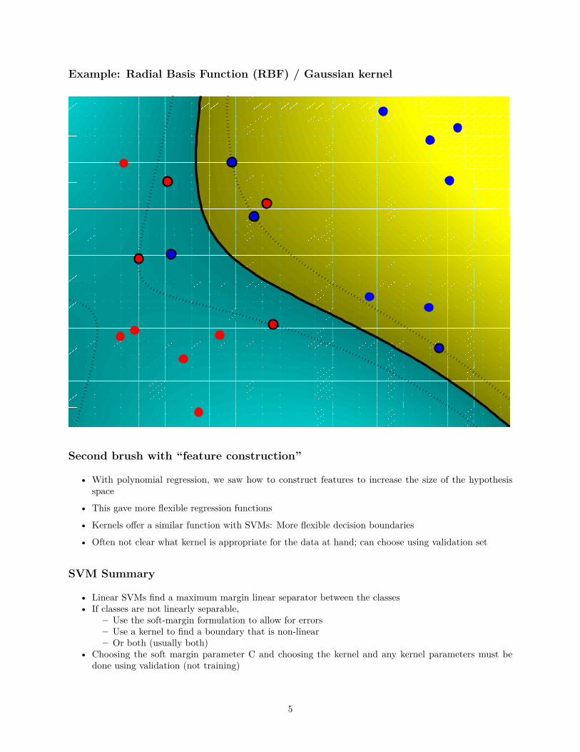
Example: Radial Basis Function (RBF) / Gaussian kernel
Second brush with “feature construction”
• With polynomial regression, we saw how to construct features to increase the size of the hypothesisspace
• This gave more flexible regression functions
• Kernels offer a similar function with SVMs: More flexible decision boundaries
• Often not clear what kernel is appropriate for the data at hand; can choose using validation set
SVM Summary
• Linear SVMs find a maximum margin linear separator between the classes• If classes are not linearly separable,
– Use the soft-margin formulation to allow for errors– Use a kernel to find a boundary that is non-linear– Or both (usually both)
• Choosing the soft margin parameter C and choosing the kernel and any kernel parameters must bedone using validation (not training)
5
Getting SVMs to work in practice
• libsvm and liblinear are popular
• Scaling the inputs (xi) is very important. (E.g. make all mean zero variance 1.)
• Two important choices:
– Kernel (and kernel parameters, e.g. γ for the RBF kernel)
– Regularization parameter C
• The parameters may interact – best C may depend on γ
• Together, these control overfitting: best to do a within-fold parameter search, using a validation set
• Clues you might be overfitting: Low margin (large weights), Large fraction of instances are supportvectors
Kernels beyond SVMs
• Remember, a kernel is a special kind of similarity measure
• A lot of research has to do with defining new kernel functions, suitable to particular tasks / kinds ofinput objects
• Many kernels are available:
– Information diffusion kernels (Lafferty and Lebanon, 2002)
– Diffusion kernels on graphs (Kondor and Jebara 2003)
– String kernels for text classification (Lodhi et al, 2002)
– String kernels for protein classification (e.g., Leslie et al, 2002)
… and others!
Instance-based learning, Decision Trees
• Non-parametric learning
• k-nearest neighbour
• Efficient implementations
• Variations
Parametric supervised learning
• So far, we have assumed that we have a data set D of labeled examples
• From this, we learn a parameter vector of a fixed size such that some error measure based on thetraining data is minimized
• These methods are called parametric, and their main goal is to summarize the data using the param-eters
• Parametric methods are typically global, i.e. have one set of parameters for the entire data space
• But what if we just remembered the data?
6

• When new instances arrive, we will compare them with what we know, and determine the answer
Non-parametric (memory-based) learning methods
• Key idea: just store all training examples ⟨xi, yi⟩
• When a query is made, compute the value of the new instance based on the values of the closest (mostsimilar) points
• Requirements:
– A distance function
– How many closest points (neighbors) to look at?
– How do we compute the value of the new point based on the existing values?
Simple idea: Connect the dots!
0.00
0.25
0.50
0.75
1.00
15 20 25
Radius.Mean
binO
utco
me
Outcome
N
R
7
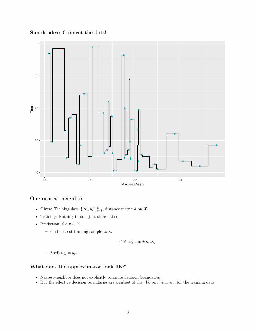
Simple idea: Connect the dots!
0
20
40
60
80
12 16 20 24
Radius.Mean
Tim
e
One-nearest neighbor
• Given: Training data {(xi, yi)}ni=1, distance metric d on X .
• Training: Nothing to do! (just store data)
• Prediction: for x ∈ X
– Find nearest training sample to x.
i∗ ∈ arg mini
d(xi, x)
– Predict y = yi∗ .
What does the approximator look like?
• Nearest-neighbor does not explicitly compute decision boundaries• But the effective decision boundaries are a subset of the Voronoi diagram for the training data
8
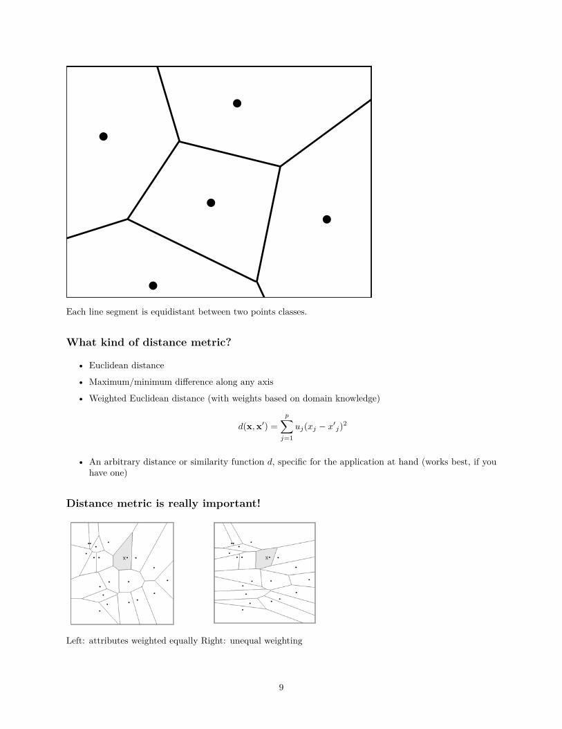
Each line segment is equidistant between two points classes.
What kind of distance metric?
• Euclidean distance
• Maximum/minimum difference along any axis
• Weighted Euclidean distance (with weights based on domain knowledge)
d(x, x′) =p∑
j=1uj(xj − x′
j)2
• An arbitrary distance or similarity function d, specific for the application at hand (works best, if youhave one)
Distance metric is really important!
!
"#$%&'()*+,+-../0+-..10+234&56+78+9##&5 :3;*<3=5>?<;54+@5<&3'3(A+B@'45+//
9C@*'D<&'<*5+E';*<3=5+95*&'=;BC$$#;5+*)5+'3$C*+D5=*#&;+F/0+F-0+GF3+<&5+*6#+4'H53;'#3<@A
!/ I+J+F// 0+F/- K+0+!- I+J+F-/ 0+F-- K+0+G!L I+J+FL/ 0+FL- K8
M35+=<3+4&<6+*)5+35<&5;*>35'()?#&+&5('#3;+'3+'3$C*+;$<=58
E';*J!'0!NK+IJF'/ O FN/K-PJQF'- O QFN-K
-E';*J!'0!NK+I+JF'/ O FN/K- P+JF'- O FN-K
-
R)5+&5@<*'D5+;=<@'3(;+'3+*)5+4';*<3=5+H5*&'=+<SS5=*+&5('#3+;)<$5;8
"#$%&'()*+,+-../0+-..10+234&56+78+9##&5 :3;*<3=5>?<;54+@5<&3'3(A+B@'45+/-
TC=@'45<3+E';*<3=5+95*&'=
M*)5&+95*&'=;G
U 9<)<@<3#?';0+V<3W>?<;540+"#&&5@<*'#3>?<;54+JB*<3S'@@P7<@*X0+9<5;Y+V'3(#+;%;*5HGK
! "
#####
$
%
&&&&&
'
(
)*
)
+)
*
*
!
"
!
!
!
#
!!
!$$
$!$
$$!
%&'()*'&'()*'%%&'(*'+
(%%&'(*'+
!
!!!!
!
!
!
"
"""
#
$$# ,
6)5&5
M&+5ZC'D<@53*@%0
Left: attributes weighted equally Right: unequal weighting
9
Distance metric tricks
• You may need to do preprocessing:
– Scale the input dimensions (or normalize them)
– Remove noisy inputs
– Determine weights for attributes based on cross-validation (or information-theoretic methods)
• Distance metric is often domain-specific
– E.g. string edit distance in bioinformatics
– E.g. trajectory distance in time series models for walking data
• Distance metric can be learned sometimes (more on this later)
k-nearest neighbor
• Given: Training data {(xi, yi)}ni=1, distance metric d on X .
• Learning: Nothing to do!
• Prediction: for x ∈ X
– Find the k nearest training samples to x.Let their indices be i1, i2, . . . , ik.
– Predict
∗ y = mean/median of {yi1 , yi2 , . . . , yik} for regression
∗ y = majority of {yi1 , yi2 , . . . , yik} for classification, or empirical probability of each class
10
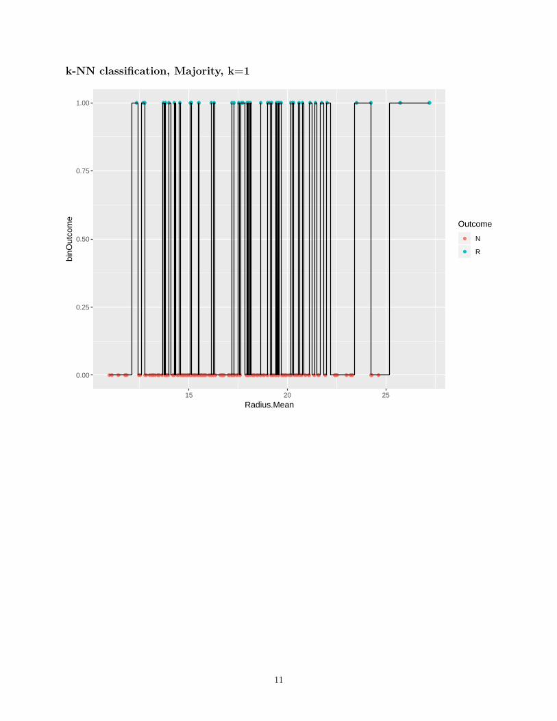
k-NN classification, Majority, k=1
0.00
0.25
0.50
0.75
1.00
15 20 25
Radius.Mean
binO
utco
me
Outcome
N
R
11
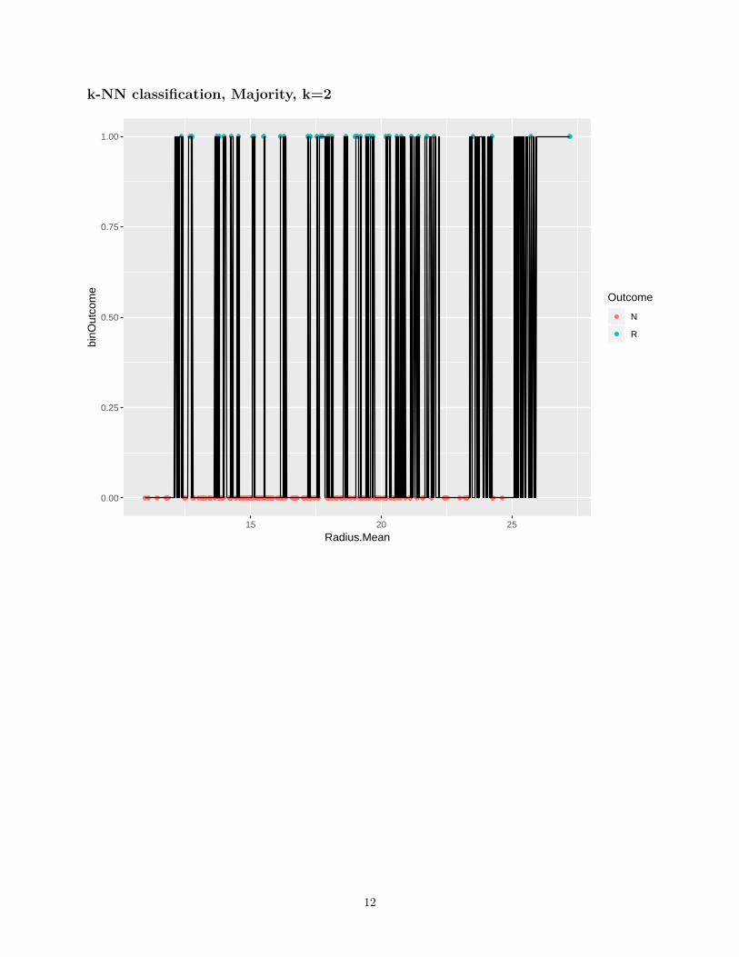
k-NN classification, Majority, k=2
0.00
0.25
0.50
0.75
1.00
15 20 25
Radius.Mean
binO
utco
me
Outcome
N
R
12
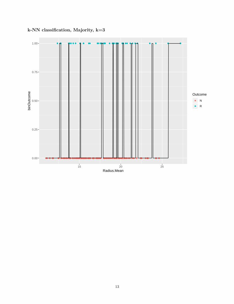
k-NN classification, Majority, k=3
0.00
0.25
0.50
0.75
1.00
15 20 25
Radius.Mean
binO
utco
me
Outcome
N
R
13
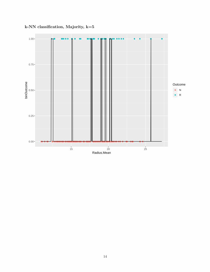
k-NN classification, Majority, k=5
0.00
0.25
0.50
0.75
1.00
15 20 25
Radius.Mean
binO
utco
me
Outcome
N
R
14
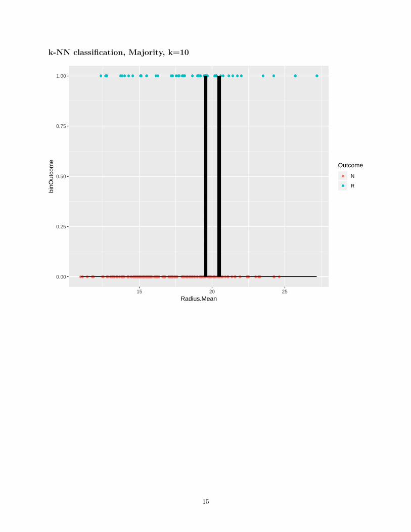
k-NN classification, Majority, k=10
0.00
0.25
0.50
0.75
1.00
15 20 25
Radius.Mean
binO
utco
me
Outcome
N
R
15
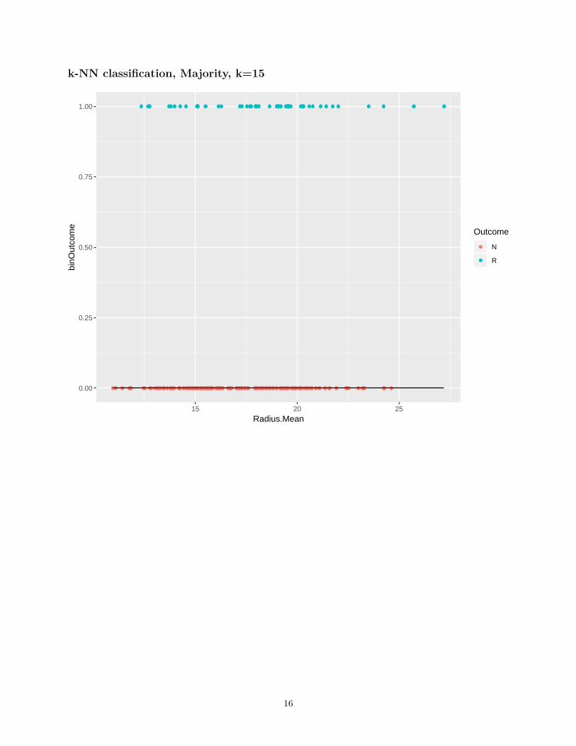
k-NN classification, Majority, k=15
0.00
0.25
0.50
0.75
1.00
15 20 25
Radius.Mean
binO
utco
me
Outcome
N
R
16
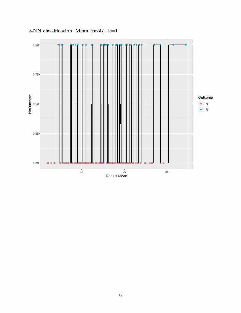
k-NN classification, Mean (prob), k=1
0.00
0.25
0.50
0.75
1.00
15 20 25
Radius.Mean
binO
utco
me
Outcome
N
R
17
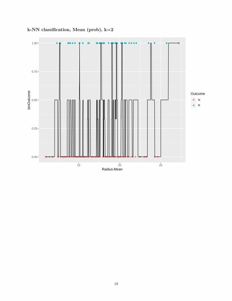
k-NN classification, Mean (prob), k=2
0.00
0.25
0.50
0.75
1.00
15 20 25
Radius.Mean
binO
utco
me
Outcome
N
R
18
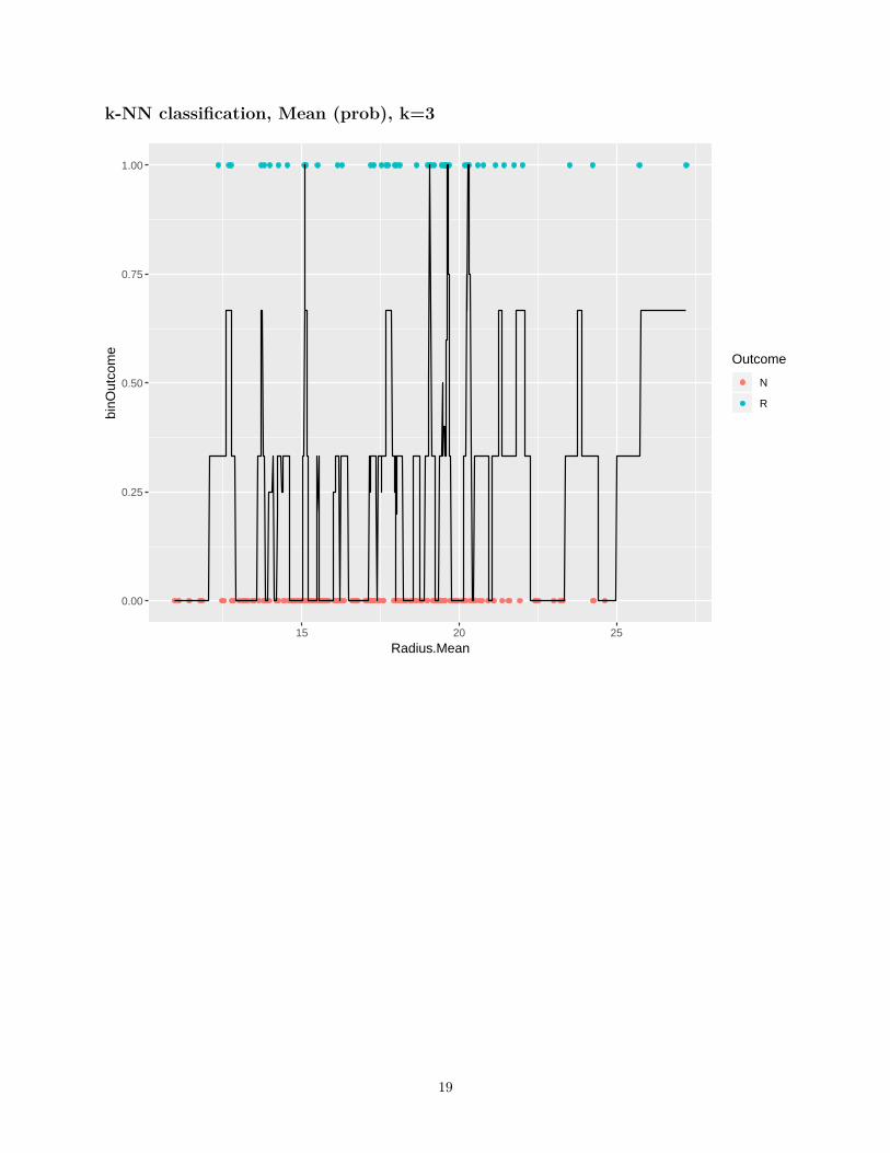
k-NN classification, Mean (prob), k=3
0.00
0.25
0.50
0.75
1.00
15 20 25
Radius.Mean
binO
utco
me
Outcome
N
R
19
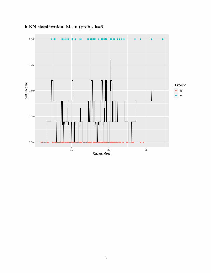
k-NN classification, Mean (prob), k=5
0.00
0.25
0.50
0.75
1.00
15 20 25
Radius.Mean
binO
utco
me
Outcome
N
R
20
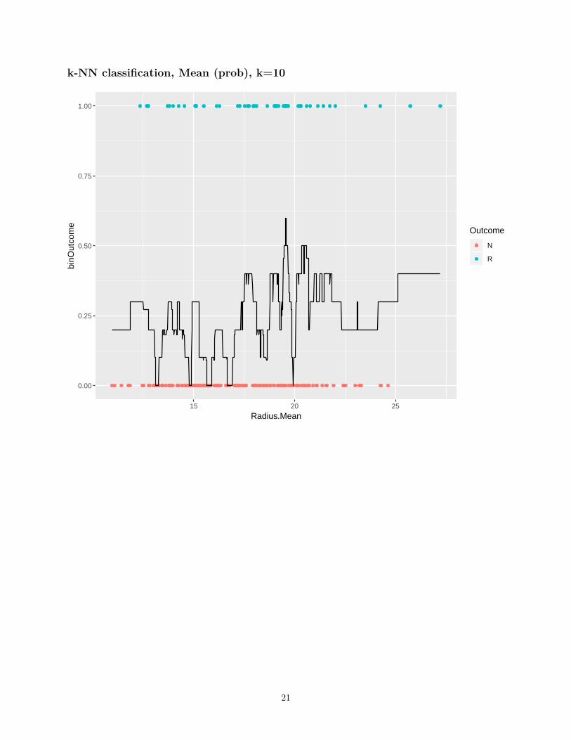
k-NN classification, Mean (prob), k=10
0.00
0.25
0.50
0.75
1.00
15 20 25
Radius.Mean
binO
utco
me
Outcome
N
R
21
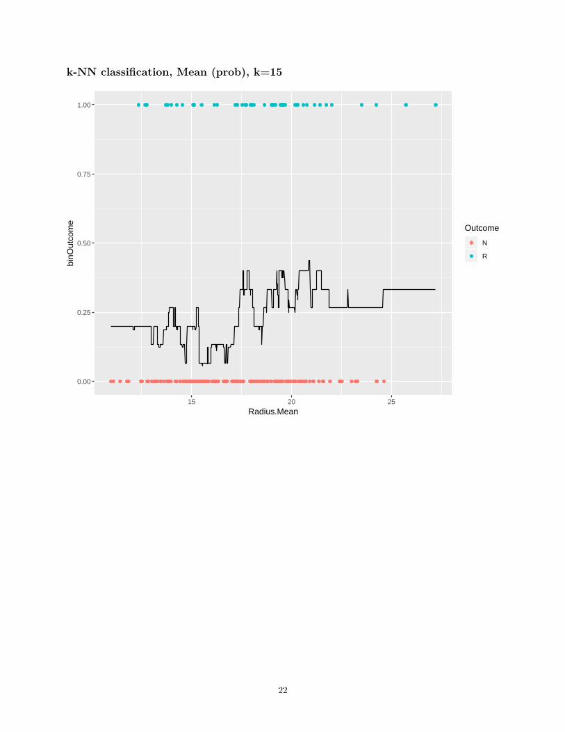
k-NN classification, Mean (prob), k=15
0.00
0.25
0.50
0.75
1.00
15 20 25
Radius.Mean
binO
utco
me
Outcome
N
R
22
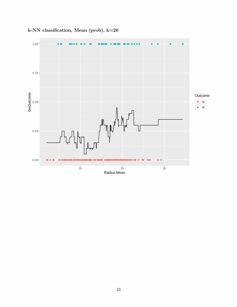
k-NN classification, Mean (prob), k=20
0.00
0.25
0.50
0.75
1.00
15 20 25
Radius.Mean
binO
utco
me
Outcome
N
R
23
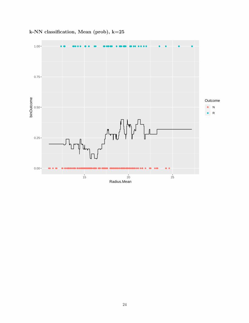
k-NN classification, Mean (prob), k=25
0.00
0.25
0.50
0.75
1.00
15 20 25
Radius.Mean
binO
utco
me
Outcome
N
R
24
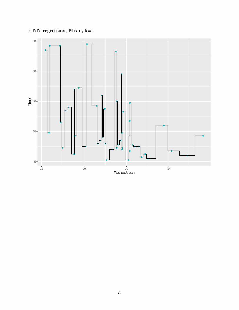
k-NN regression, Mean, k=1
0
20
40
60
80
12 16 20 24
Radius.Mean
Tim
e
25
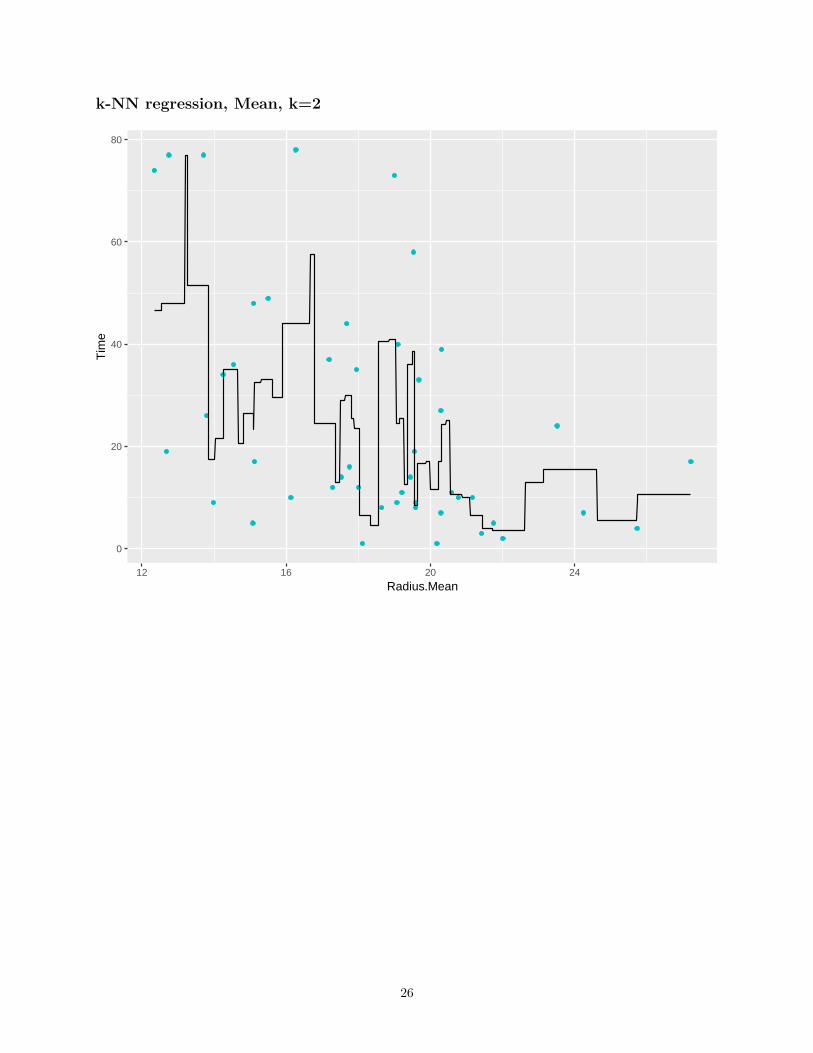
k-NN regression, Mean, k=2
0
20
40
60
80
12 16 20 24
Radius.Mean
Tim
e
26
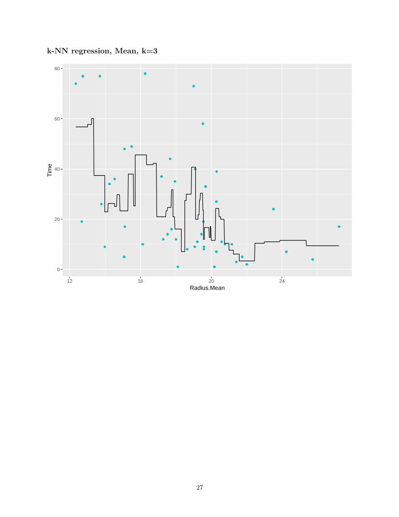
k-NN regression, Mean, k=3
0
20
40
60
80
12 16 20 24
Radius.Mean
Tim
e
27
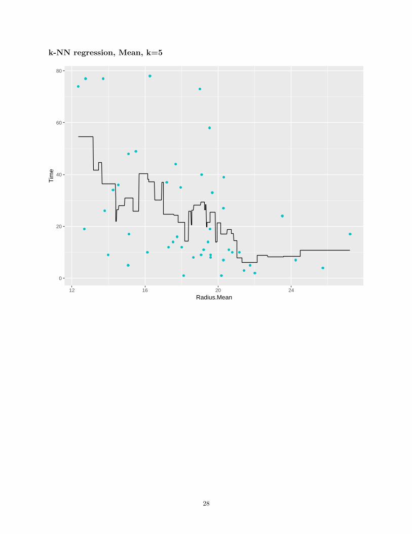
k-NN regression, Mean, k=5
0
20
40
60
80
12 16 20 24
Radius.Mean
Tim
e
28
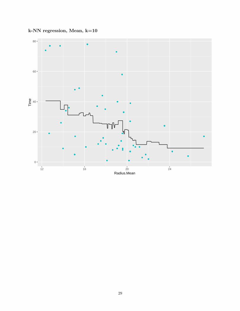
k-NN regression, Mean, k=10
0
20
40
60
80
12 16 20 24
Radius.Mean
Tim
e
29
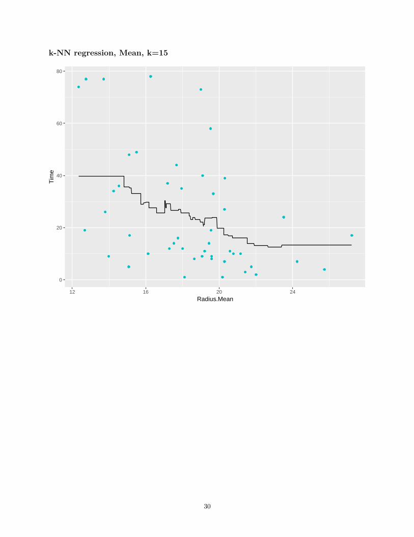
k-NN regression, Mean, k=15
0
20
40
60
80
12 16 20 24
Radius.Mean
Tim
e
30
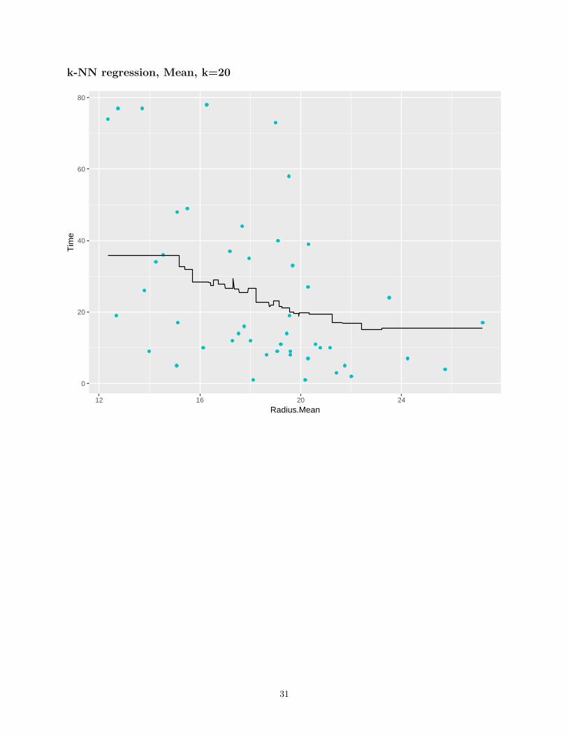
k-NN regression, Mean, k=20
0
20
40
60
80
12 16 20 24
Radius.Mean
Tim
e
31
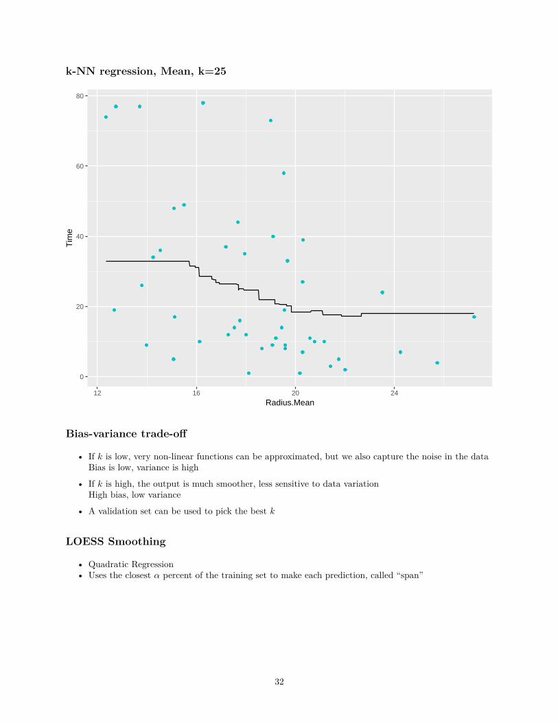
k-NN regression, Mean, k=25
0
20
40
60
80
12 16 20 24
Radius.Mean
Tim
e
Bias-variance trade-off
• If k is low, very non-linear functions can be approximated, but we also capture the noise in the dataBias is low, variance is high
• If k is high, the output is much smoother, less sensitive to data variationHigh bias, low variance
• A validation set can be used to pick the best k
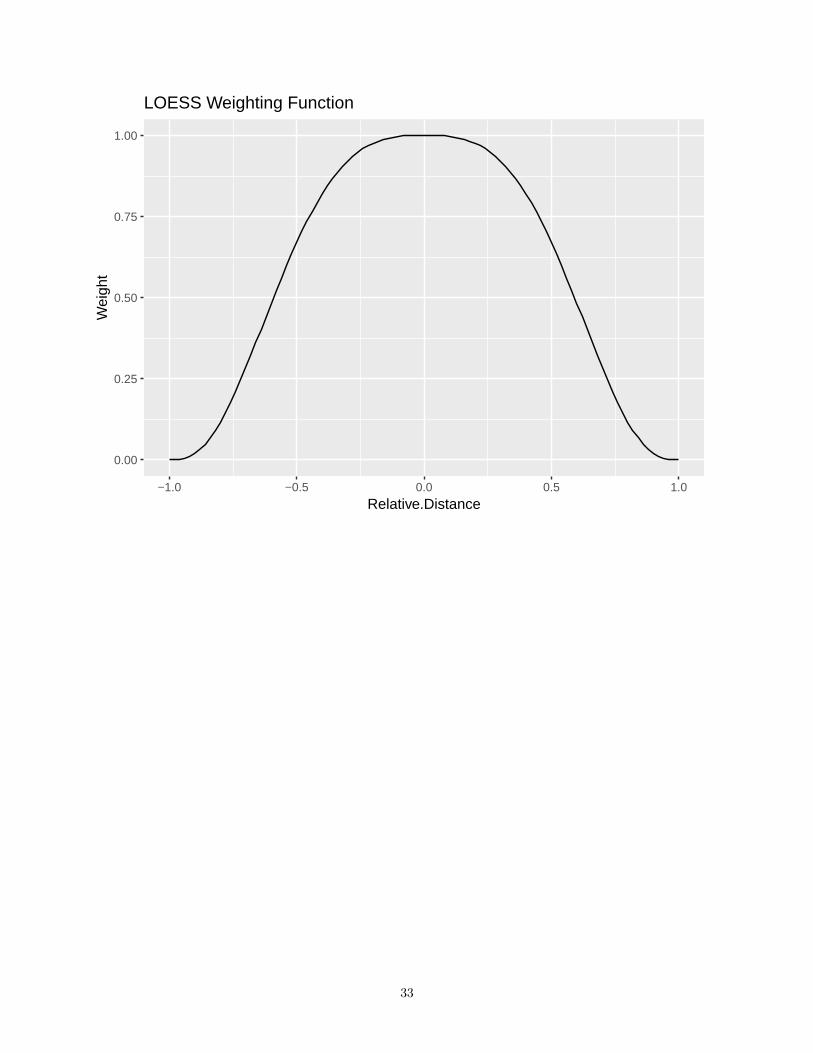
LOESS Smoothing
• Quadratic Regression• Uses the closest α percent of the training set to make each prediction, called “span”
32
0.00
0.25
0.50
0.75
1.00
−1.0 −0.5 0.0 0.5 1.0
Relative.Distance
Wei
ght
LOESS Weighting Function
33
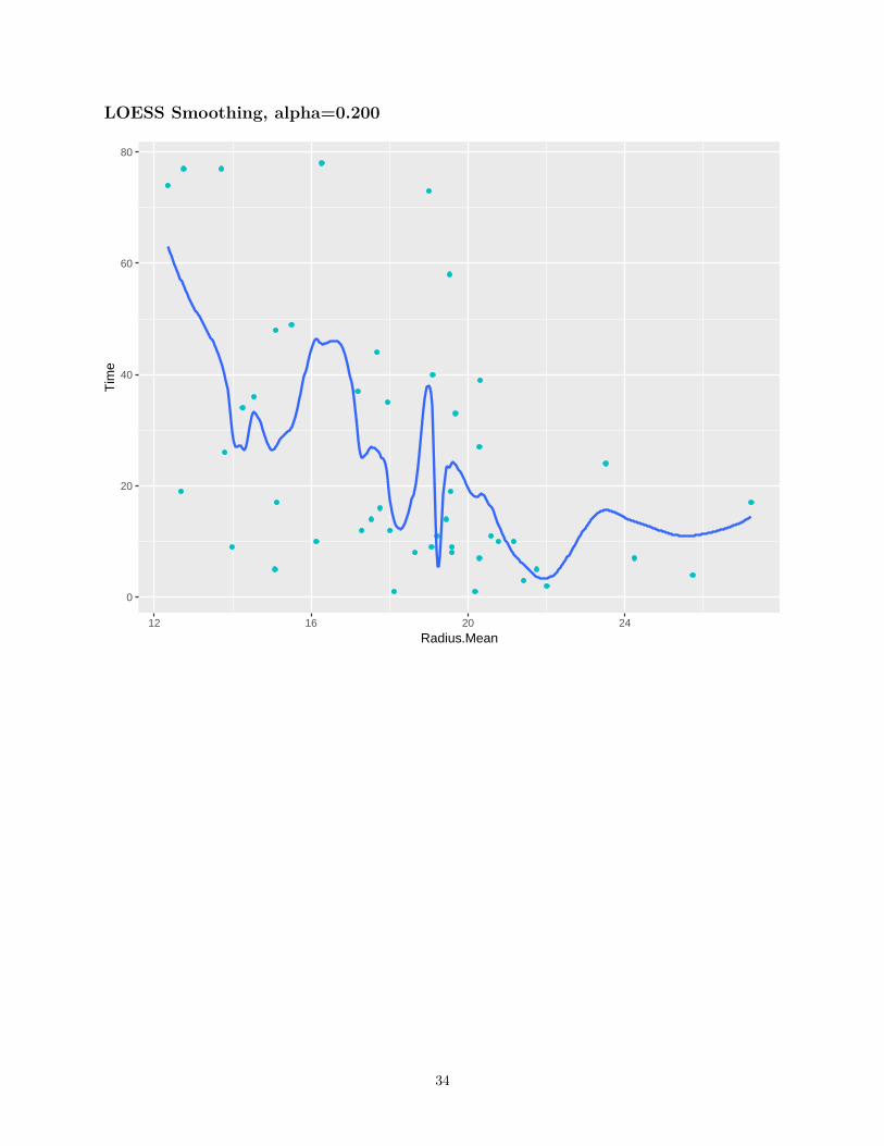
LOESS Smoothing, alpha=0.200
0
20
40
60
80
12 16 20 24
Radius.Mean
Tim
e
34
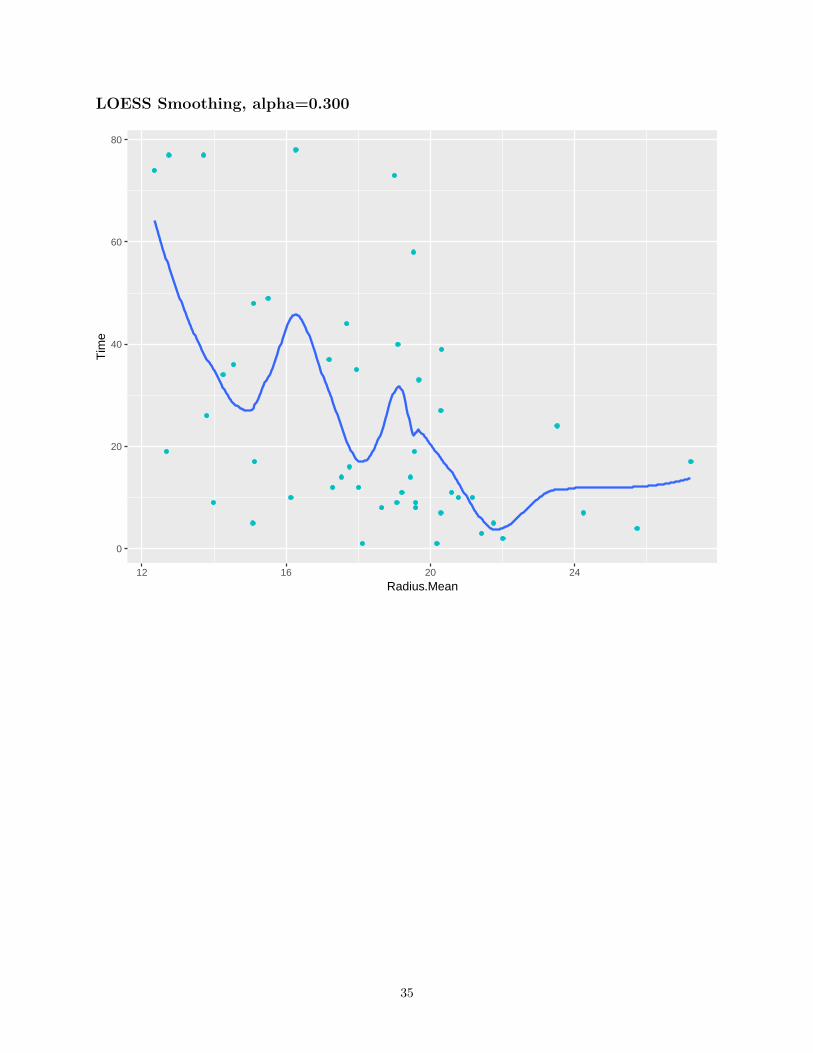
LOESS Smoothing, alpha=0.300
0
20
40
60
80
12 16 20 24
Radius.Mean
Tim
e
35
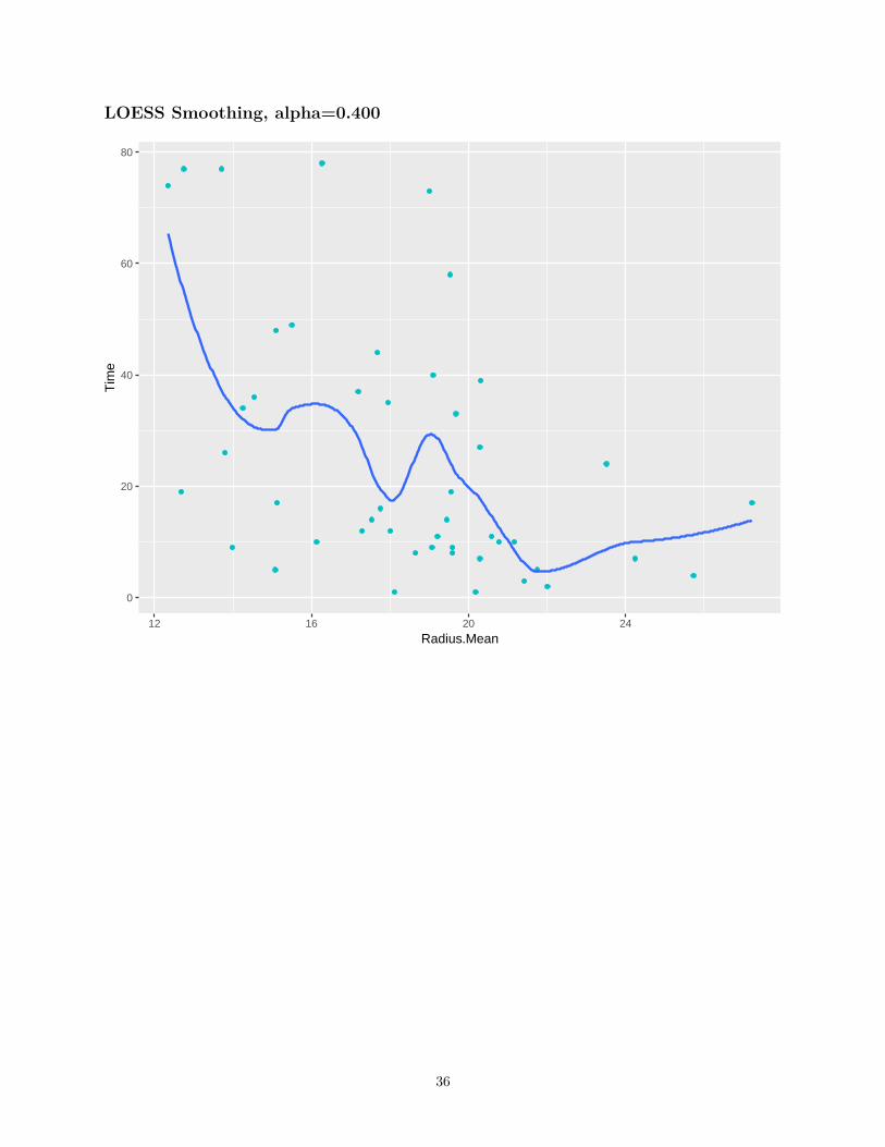
LOESS Smoothing, alpha=0.400
0
20
40
60
80
12 16 20 24
Radius.Mean
Tim
e
36
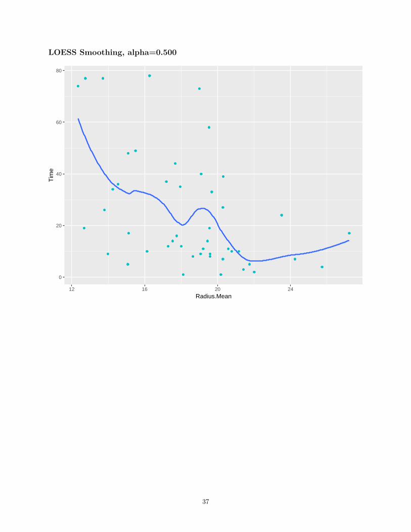
LOESS Smoothing, alpha=0.500
0
20
40
60
80
12 16 20 24
Radius.Mean
Tim
e
37
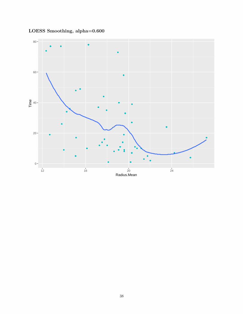
LOESS Smoothing, alpha=0.600
0
20
40
60
80
12 16 20 24
Radius.Mean
Tim
e
38

LOESS Smoothing, alpha=0.700
0
20
40
60
80
12 16 20 24
Radius.Mean
Tim
e
39

LOESS Smoothing, alpha=0.750
0
20
40
60
80
12 16 20 24
Radius.Mean
Tim
e
40
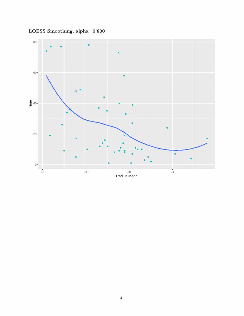
LOESS Smoothing, alpha=0.800
0
20
40
60
80
12 16 20 24
Radius.Mean
Tim
e
41
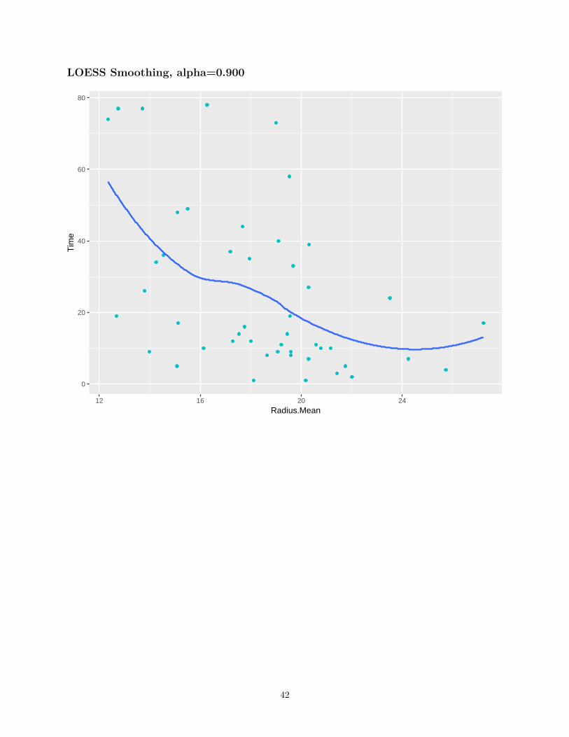
LOESS Smoothing, alpha=0.900
0
20
40
60
80
12 16 20 24
Radius.Mean
Tim
e
42
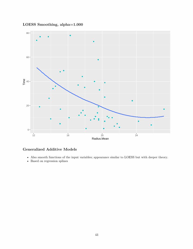
LOESS Smoothing, alpha=1.000
0
20
40
60
80
12 16 20 24
Radius.Mean
Tim
e
Generalized Additive Models
• Also smooth functions of the input variables; appearance similar to LOESS but with deeper theory.• Based on regression splines
43
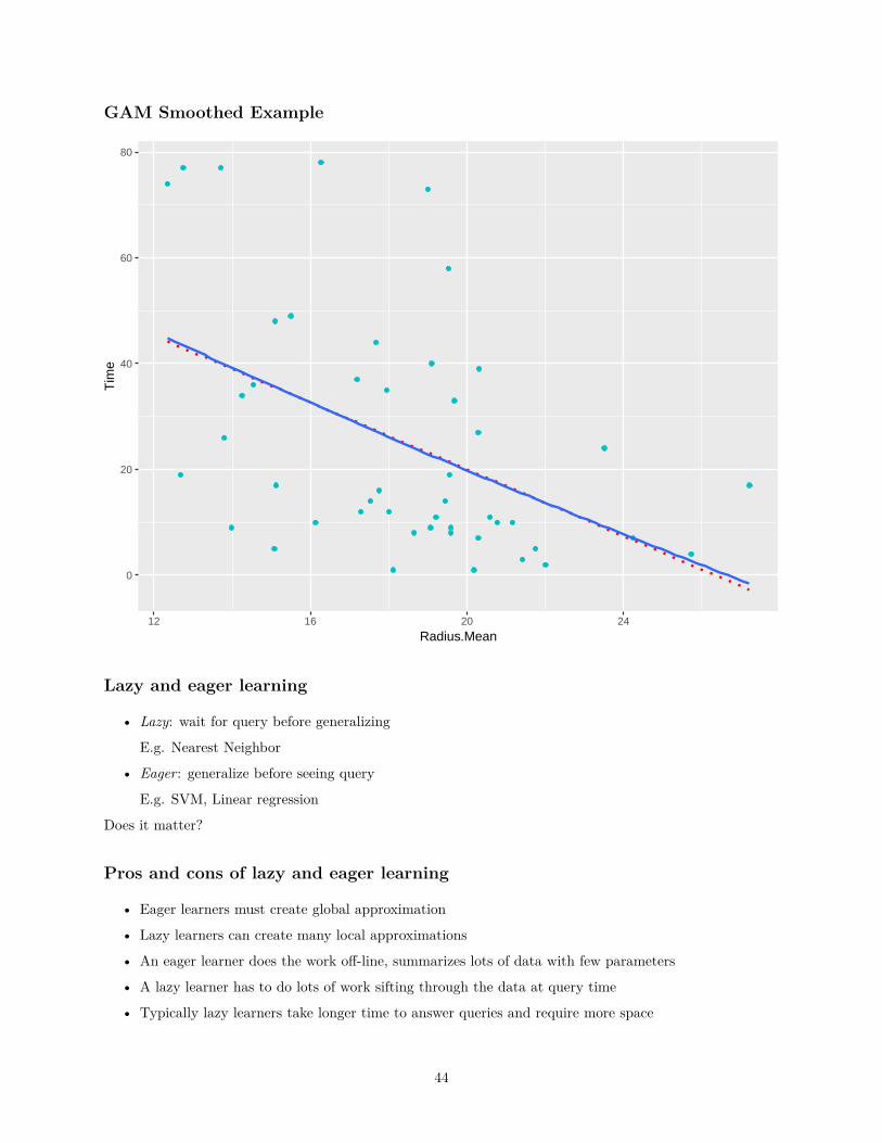
GAM Smoothed Example
0
20
40
60
80
12 16 20 24
Radius.Mean
Tim
e
Lazy and eager learning
• Lazy: wait for query before generalizing
E.g. Nearest Neighbor
• Eager: generalize before seeing query
E.g. SVM, Linear regression
Does it matter?
Pros and cons of lazy and eager learning
• Eager learners must create global approximation
• Lazy learners can create many local approximations
• An eager learner does the work off-line, summarizes lots of data with few parameters
• A lazy learner has to do lots of work sifting through the data at query time
• Typically lazy learners take longer time to answer queries and require more space
44
When to consider nonparametric methods
• When you have: instances that map to points in Rp, not too many attributes per instance (< 20), lotsof data
• Advantages:
– Training is very fast
– Easy to learn complex functions over few variables
– Can give back confidence intervals in addition to the prediction
– Often wins if you have enough data
• Disadvantages:
– Slow at query time
– Query answering complexity depends on the number of instances
– Easily fooled by irrelevant attributes (for most distance metrics)
– “Inference” is not possible
Decision Trees
• What are decision trees?
• Methods for constructing decision trees
• Overfitting avoidance
Non-metric learning
• The result of learning is not a set of parameters, but there is no distance metric to assess similarityof different instances
• Typical examples:
– Decision trees
– Rule-based systems
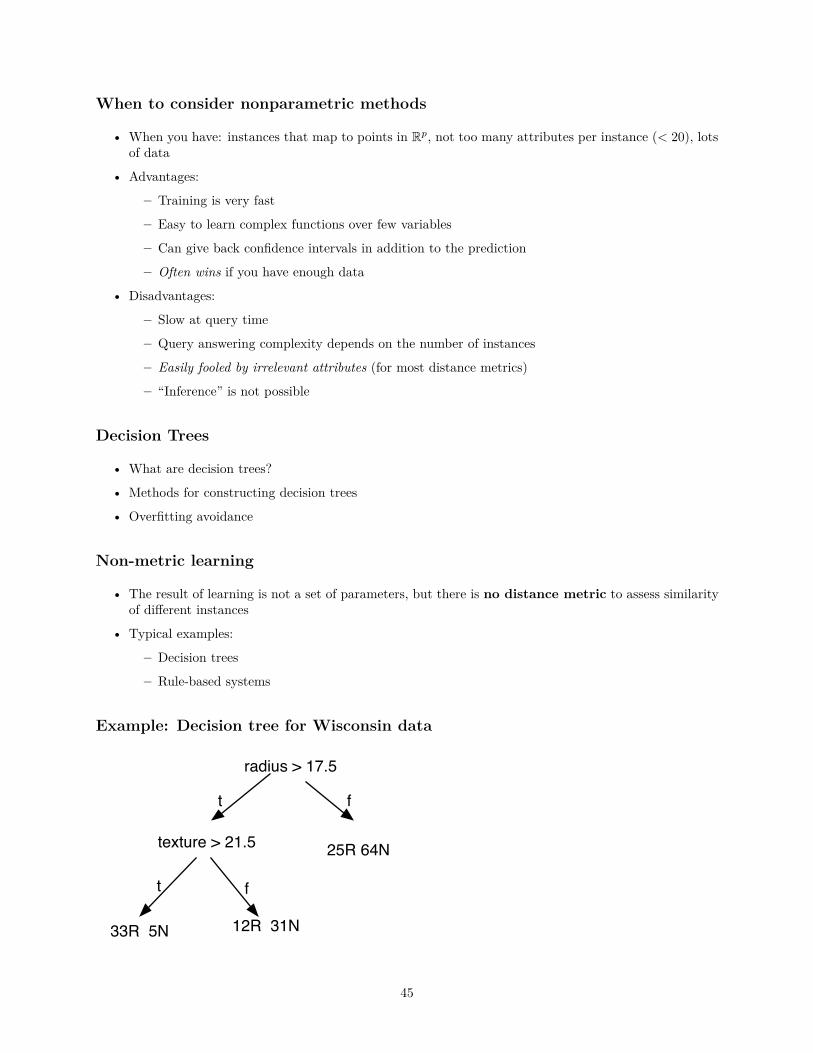
Example: Decision tree for Wisconsin data
radius > 17.5
texture > 21.5
t f
t f
33R 5N 12R 31N
25R 64N
45
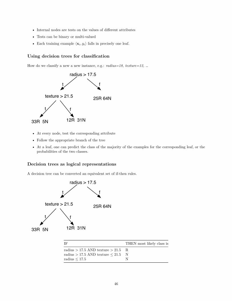
• Internal nodes are tests on the values of different attributes
• Tests can be binary or multi-valued
• Each training example ⟨xi, yi⟩ falls in precisely one leaf.
Using decision trees for classification
How do we classify a new a new instance, e.g.: radius=18, texture=12, …
radius > 17.5
texture > 21.5
t f
t f
33R 5N 12R 31N
25R 64N
• At every node, test the corresponding attribute
• Follow the appropriate branch of the tree
• At a leaf, one can predict the class of the majority of the examples for the corresponding leaf, or theprobabilities of the two classes.
Decision trees as logical representations
A decision tree can be converted an equivalent set of if-then rules.
radius > 17.5
texture > 21.5
t f
t f
33R 5N 12R 31N
25R 64N
IF THEN most likely class isradius > 17.5 AND texture > 21.5 Rradius > 17.5 AND texture ≤ 21.5 Nradius ≤ 17.5 N
46
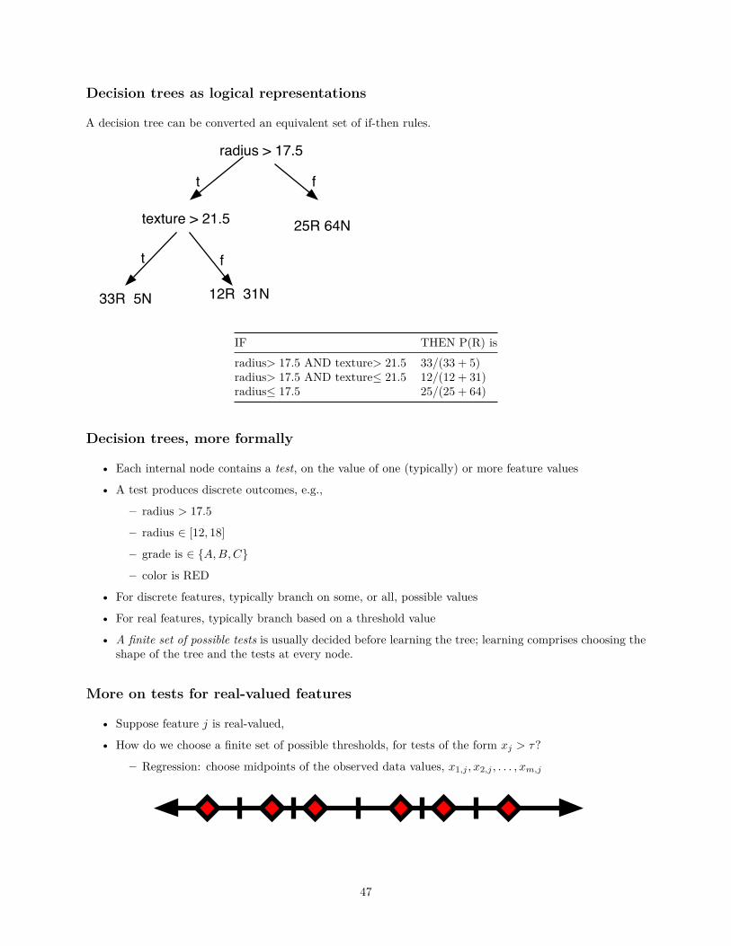
Decision trees as logical representations
A decision tree can be converted an equivalent set of if-then rules.
radius > 17.5
texture > 21.5
t f
t f
33R 5N 12R 31N
25R 64N
IF THEN P(R) isradius> 17.5 AND texture> 21.5 33/(33 + 5)radius> 17.5 AND texture≤ 21.5 12/(12 + 31)radius≤ 17.5 25/(25 + 64)
Decision trees, more formally
• Each internal node contains a test, on the value of one (typically) or more feature values
• A test produces discrete outcomes, e.g.,
– radius > 17.5
– radius ∈ [12, 18]
– grade is ∈ {A, B, C}
– color is RED
• For discrete features, typically branch on some, or all, possible values
• For real features, typically branch based on a threshold value
• A finite set of possible tests is usually decided before learning the tree; learning comprises choosing theshape of the tree and the tests at every node.
More on tests for real-valued features
• Suppose feature j is real-valued,
• How do we choose a finite set of possible thresholds, for tests of the form xj > τ?
– Regression: choose midpoints of the observed data values, x1,j , x2,j , . . . , xm,j
47
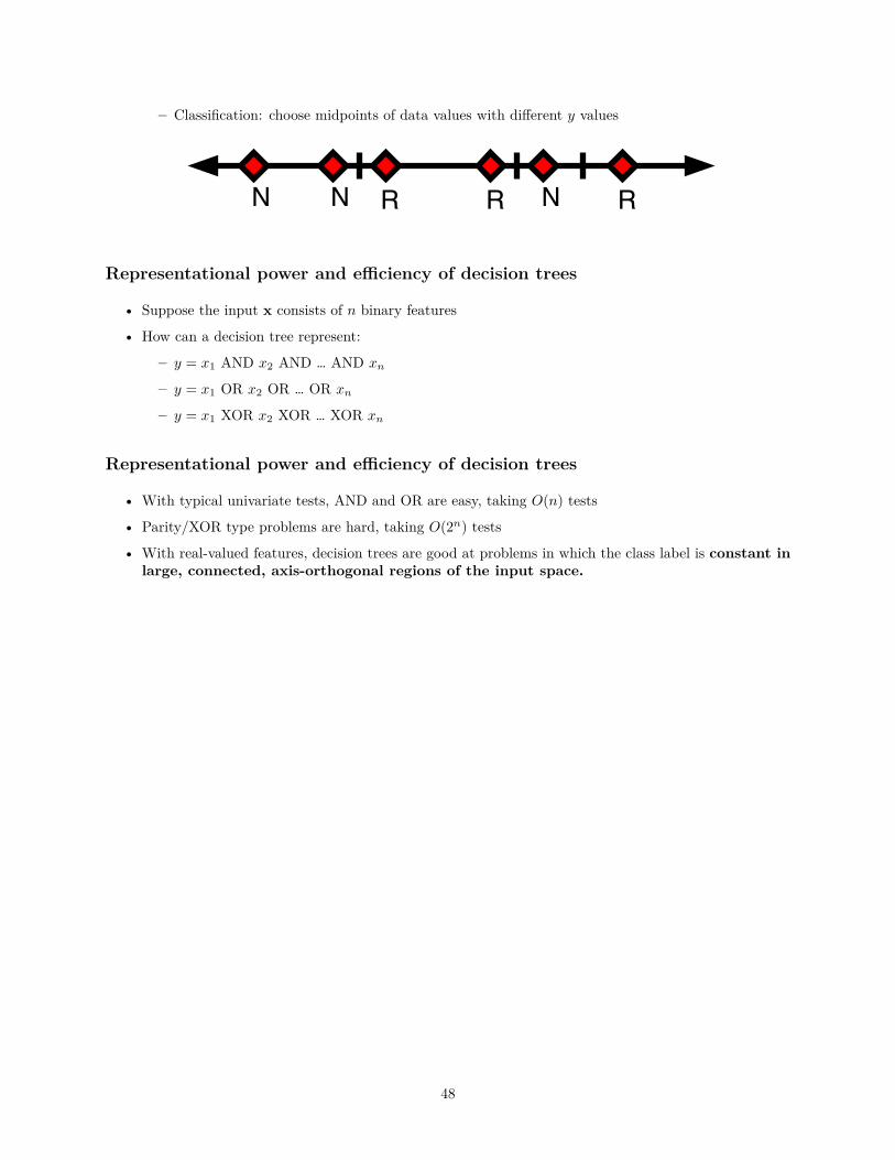
– Classification: choose midpoints of data values with different y values
N RR RN N
Representational power and efficiency of decision trees
• Suppose the input x consists of n binary features
• How can a decision tree represent:
– y = x1 AND x2 AND … AND xn
– y = x1 OR x2 OR … OR xn
– y = x1 XOR x2 XOR … XOR xn
Representational power and efficiency of decision trees
• With typical univariate tests, AND and OR are easy, taking O(n) tests
• Parity/XOR type problems are hard, taking O(2n) tests
• With real-valued features, decision trees are good at problems in which the class label is constant inlarge, connected, axis-orthogonal regions of the input space.
48
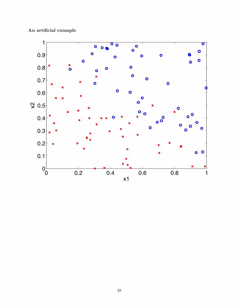
An artificial example
0 0.2 0.4 0.6 0.8 10
0.1
0.2
0.3
0.4
0.5
0.6
0.7
0.8
0.9
1
x1
x2
49
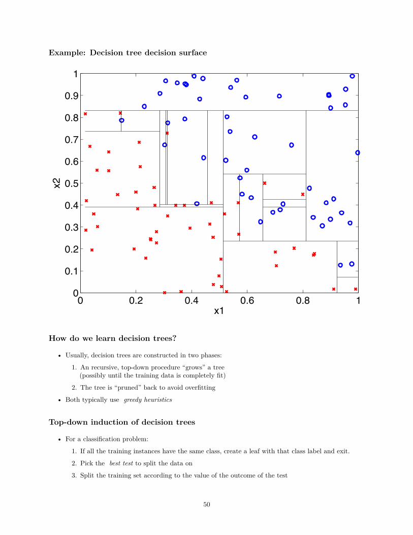
Example: Decision tree decision surface
0 0.2 0.4 0.6 0.8 10
0.1
0.2
0.3
0.4
0.5
0.6
0.7
0.8
0.9
1
x1
x2
How do we learn decision trees?
• Usually, decision trees are constructed in two phases:
1. An recursive, top-down procedure “grows” a tree(possibly until the training data is completely fit)
2. The tree is “pruned” back to avoid overfitting
• Both typically use greedy heuristics
Top-down induction of decision trees
• For a classification problem:
1. If all the training instances have the same class, create a leaf with that class label and exit.
2. Pick the best test to split the data on
3. Split the training set according to the value of the outcome of the test
50
4. Recurse on each subset of the training data
Top-down induction of decision trees
• For a regression problem - same as above, except:
– The decision on when to stop splitting has to be made earlier
– At a leaf, either predict the mean value, or do a linear fit
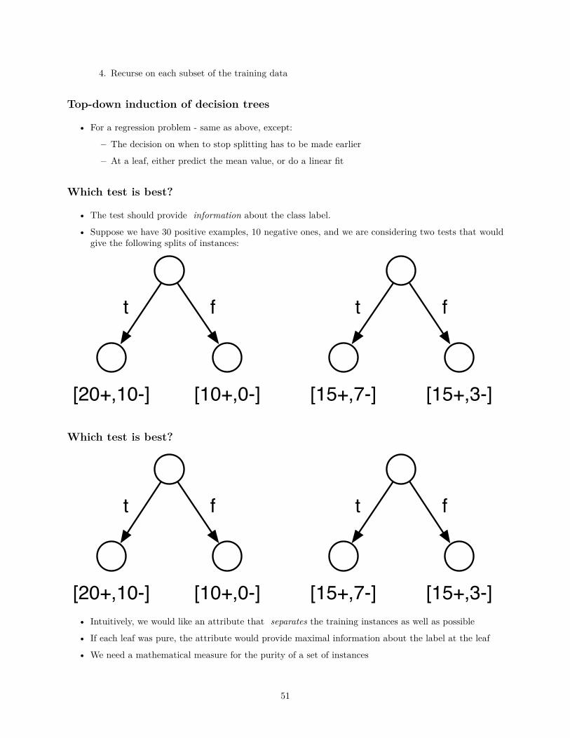
Which test is best?
• The test should provide information about the class label.
• Suppose we have 30 positive examples, 10 negative ones, and we are considering two tests that wouldgive the following splits of instances:
t f
[20+,10-] [10+,0-]
t f
[15+,7-] [15+,3-]
Which test is best?
t f
[20+,10-] [10+,0-]
t f
[15+,7-] [15+,3-]• Intuitively, we would like an attribute that separates the training instances as well as possible
• If each leaf was pure, the attribute would provide maximal information about the label at the leaf
• We need a mathematical measure for the purity of a set of instances
51
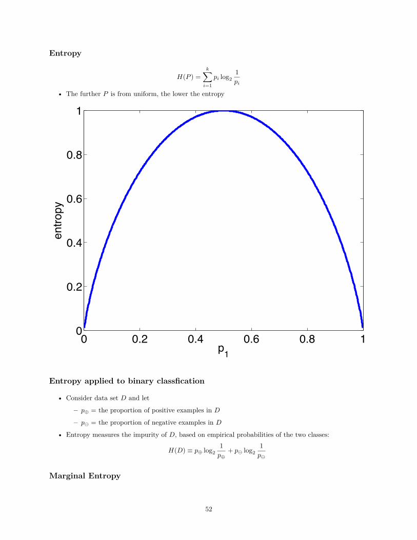
Entropy
H(P ) =k∑
i=1pi log2
1pi
• The further P is from uniform, the lower the entropy
0 0.2 0.4 0.6 0.8 10
0.2
0.4
0.6
0.8
1
p1
entropy
Entropy applied to binary classfication
• Consider data set D and let
– p⊕ = the proportion of positive examples in D
– p⊖ = the proportion of negative examples in D
• Entropy measures the impurity of D, based on empirical probabilities of the two classes:
H(D) ≡ p⊕ log21
p⊕+ p⊖ log2
1p⊖
Marginal Entropy
52
x =HasKids y =OwnsFrozenVideoYes YesYes YesYes YesYes YesNo NoNo NoYes NoYes No
• From the table, we can estimate P (Y = Yes) = 0.5 = P (Y = No).
• Thus, we estimate H(Y ) = 0.5 log 10.5 + 0.5 log 1
0.5 = 1.
Specific Conditional entropy
x =HasKids y =OwnsFrozenVideoYes YesYes YesYes YesYes YesNo NoNo NoYes NoYes No
Specific conditional entropy is the uncertainty in Y given a particular x value. E.g.,
• P (Y = Yes|X = Yes) = 23 , P (Y = No|X = Yes) = 1
3
• H(Y |X = Yes) = 23 log 1
( 23 ) + 1
3 log 1( 1
3 ) ≈ 0.9183.
(Average) Conditional entropy
x =HasKids y =OwnsFrozenVideoYes YesYes YesYes YesYes YesNo NoNo NoYes NoYes No
• The conditional entropy, H(Y |X), is the specific conditional entropy of y averaged over the values forx:
H(Y |X) =∑
x
P (X = x)H(Y |X = x)
53
• H(Y |X = Yes) = 23 log 1
( 23 ) + 1
3 log 1( 1
3 ) ≈ 0.9183
• H(Y |X = No) = 0 log 10 + 1 log 1
1 = 0.
• H(Y |X) = H(Y |X = Yes)P (X = Yes) + H(Y |X = No)P (X = No) = 0.9183 · 34 + 0 · 1
4 ≈ 0.6887
• Interpretation: the expected number of bits needed to transmit y if both the emitter and the receiverknow the possible values of x (but before they are told x’s specific value).
Information gain
• How much does the entropy of Y go down, on average, if I am told the value of X?
IG(Y |X) = H(Y ) − H(Y |X)
This is called information gain
• Alternative interpretation: what reduction in entropy would be obtained by knowing X
• Intuitively, this has the meaning we seek for decision tree construction
Previous example: H(Y ) = 1, E[H(Y |X)] = 0.6887, so I.G. is 0.3113
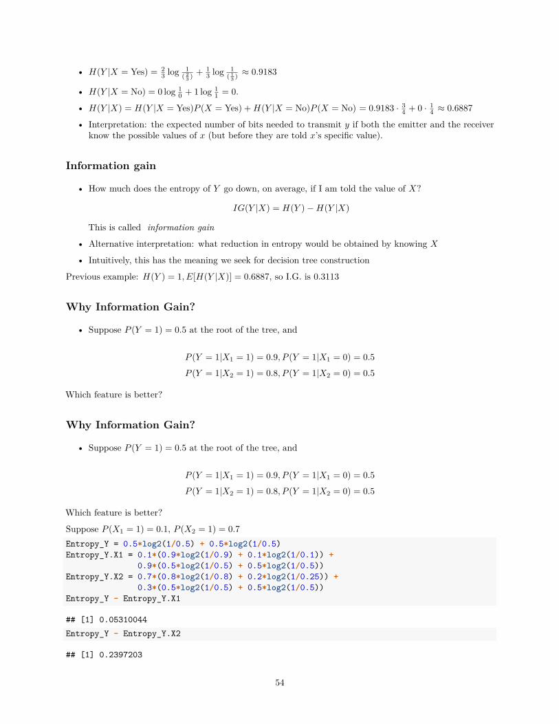
Why Information Gain?
• Suppose P (Y = 1) = 0.5 at the root of the tree, and
P (Y = 1|X1 = 1) = 0.9, P (Y = 1|X1 = 0) = 0.5
P (Y = 1|X2 = 1) = 0.8, P (Y = 1|X2 = 0) = 0.5
Which feature is better?
Why Information Gain?
• Suppose P (Y = 1) = 0.5 at the root of the tree, and
P (Y = 1|X1 = 1) = 0.9, P (Y = 1|X1 = 0) = 0.5
P (Y = 1|X2 = 1) = 0.8, P (Y = 1|X2 = 0) = 0.5
Which feature is better?
Suppose P (X1 = 1) = 0.1, P (X2 = 1) = 0.7Entropy_Y = 0.5*log2(1/0.5) + 0.5*log2(1/0.5)Entropy_Y.X1 = 0.1*(0.9*log2(1/0.9) + 0.1*log2(1/0.1)) +
0.9*(0.5*log2(1/0.5) + 0.5*log2(1/0.5))Entropy_Y.X2 = 0.7*(0.8*log2(1/0.8) + 0.2*log2(1/0.25)) +
0.3*(0.5*log2(1/0.5) + 0.5*log2(1/0.5))Entropy_Y - Entropy_Y.X1
## [1] 0.05310044Entropy_Y - Entropy_Y.X2
## [1] 0.2397203
54
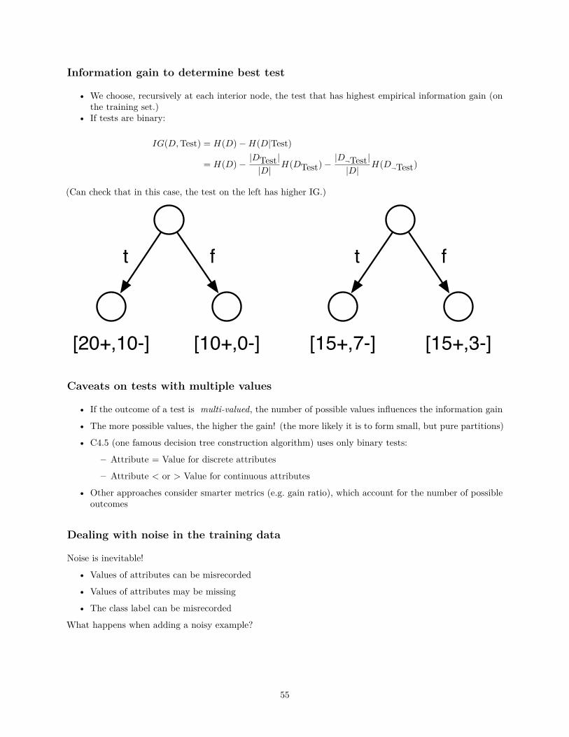
Information gain to determine best test
• We choose, recursively at each interior node, the test that has highest empirical information gain (onthe training set.)
• If tests are binary:
IG(D, Test) = H(D) − H(D|Test)
= H(D) −|DTest|
|D|H(DTest) −
|D¬Test||D|
H(D¬Test)
(Can check that in this case, the test on the left has higher IG.)
t f
[20+,10-] [10+,0-]
t f
[15+,7-] [15+,3-]
Caveats on tests with multiple values
• If the outcome of a test is multi-valued, the number of possible values influences the information gain
• The more possible values, the higher the gain! (the more likely it is to form small, but pure partitions)
• C4.5 (one famous decision tree construction algorithm) uses only binary tests:
– Attribute = Value for discrete attributes
– Attribute < or > Value for continuous attributes
• Other approaches consider smarter metrics (e.g. gain ratio), which account for the number of possibleoutcomes
Dealing with noise in the training data
Noise is inevitable!
• Values of attributes can be misrecorded
• Values of attributes may be missing
• The class label can be misrecorded
What happens when adding a noisy example?
55
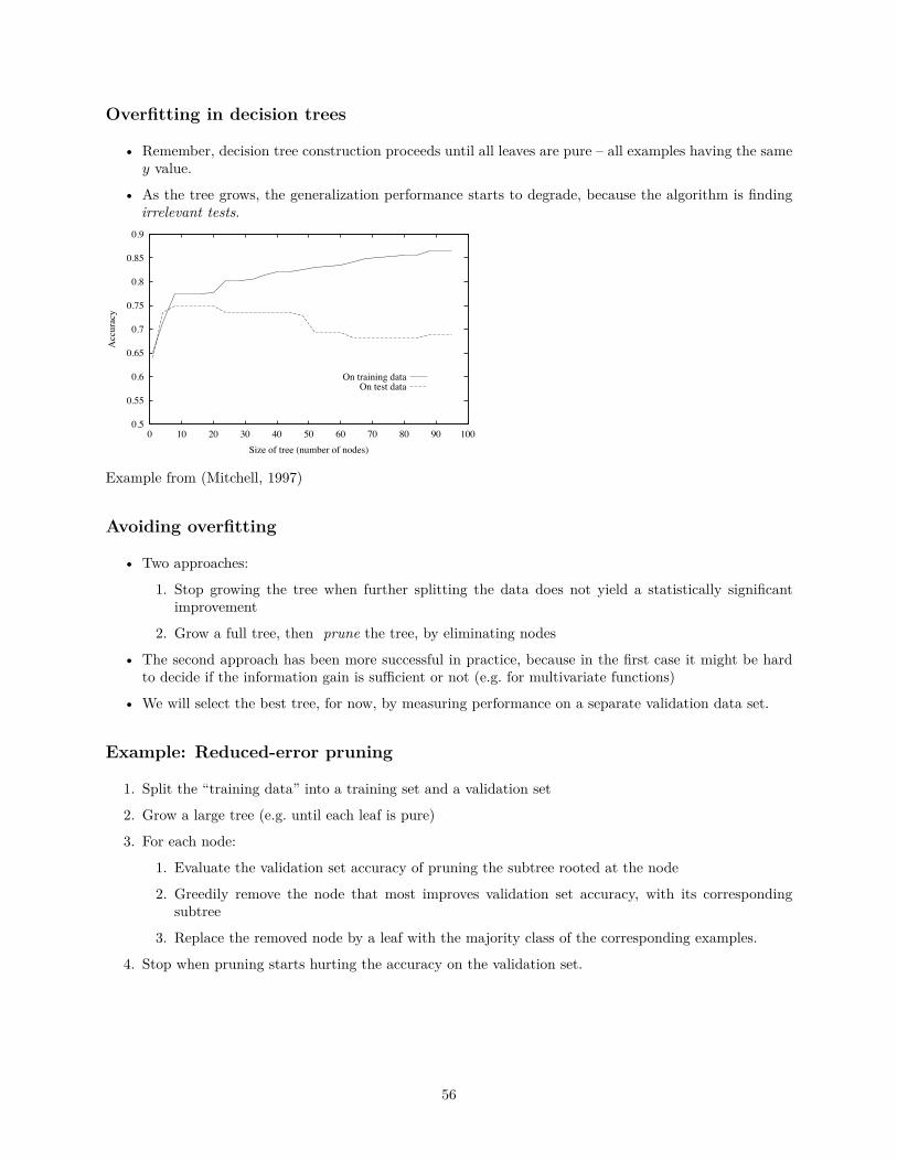
Overfitting in decision trees
• Remember, decision tree construction proceeds until all leaves are pure – all examples having the samey value.
• As the tree grows, the generalization performance starts to degrade, because the algorithm is findingirrelevant tests.
0.5
0.55
0.6
0.65
0.7
0.75
0.8
0.85
0.9
0 10 20 30 40 50 60 70 80 90 100
Acc
urac
y
Size of tree (number of nodes)
On training dataOn test data
Example from (Mitchell, 1997)
Avoiding overfitting
• Two approaches:
1. Stop growing the tree when further splitting the data does not yield a statistically significantimprovement
2. Grow a full tree, then prune the tree, by eliminating nodes
• The second approach has been more successful in practice, because in the first case it might be hardto decide if the information gain is sufficient or not (e.g. for multivariate functions)
• We will select the best tree, for now, by measuring performance on a separate validation data set.
Example: Reduced-error pruning
1. Split the “training data” into a training set and a validation set
2. Grow a large tree (e.g. until each leaf is pure)
3. For each node:
1. Evaluate the validation set accuracy of pruning the subtree rooted at the node
2. Greedily remove the node that most improves validation set accuracy, with its correspondingsubtree
3. Replace the removed node by a leaf with the majority class of the corresponding examples.
4. Stop when pruning starts hurting the accuracy on the validation set.
56
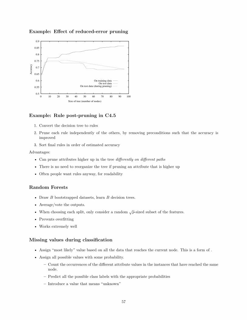
Example: Effect of reduced-error pruning
0.5
0.55
0.6
0.65
0.7
0.75
0.8
0.85
0.9
0 10 20 30 40 50 60 70 80 90 100
Acc
urac
y
Size of tree (number of nodes)
On training dataOn test data
On test data (during pruning)
Example: Rule post-pruning in C4.5
1. Convert the decision tree to rules
2. Prune each rule independently of the others, by removing preconditions such that the accuracy isimproved
3. Sort final rules in order of estimated accuracy
Advantages:
• Can prune attributes higher up in the tree differently on different paths
• There is no need to reorganize the tree if pruning an attribute that is higher up
• Often people want rules anyway, for readability
Random Forests
• Draw B bootstrapped datasets, learn B decision trees.
• Average/vote the outputs.
• When choosing each split, only consider a random √p-sized subset of the features.
• Prevents overfitting
• Works extremely well
Missing values during classification
• Assign “most likely” value based on all the data that reaches the current node. This is a form of .
• Assign all possible values with some probability.
– Count the occurrences of the different attribute values in the instances that have reached the samenode.
– Predict all the possible class labels with the appropriate probabilities
– Introduce a value that means “unknown”
57
Decision Tree Summary (1)
• Very fast learning algorithms (e.g. C4.5, CART)
• Attributes may be discrete or continuous, no preprocessing needed
• Provide a general representation of classification rules
• Easy to understand! Though…
– Exact tree output may be sensitive to small changes in data
– With many features, tests may not be meaningful
Decision Tree Summary (2)
• In standard form, good for (nonlinear) piecewise axis-orthogonal decision boundaries – not good withsmooth, curvilinear boundaries
• In regression, the function obtained is discontinuous, which may not be desirable
• Good accuracy in practice – many applications
58


![arXiv:1201.2648v4 [cond-mat.str-el] 16 Sep 2014 · 2014-09-17 · Symmetry-protected topological orders for interacting fermions { Fermionic topological nonlinear ˙ models and a](https://static.fdocument.org/doc/165x107/5f70160faf2ad47813162637/arxiv12012648v4-cond-matstr-el-16-sep-2014-2014-09-17-symmetry-protected.jpg)