Nonlinear dynamics

Yichao Jing

OutlineØ Examples for nonlinearities in particle accelerator

Ø Approaches to study nonlinear resonances

Ø Chromaticity, resonance driving terms and dynamic aperture

Nonlineardynamics

Nonlinearities in accelerator

ρρρ

ρρ

BBsK

BBsK

BBysKy

BB

xsKx

yx

xy

yx

112 )( ,1)(

)( ,)(

±==

Δ=+ʹ́

Δ±=+ʹ́

!

!

δ = ω0

2πβ 2EeV (sinφ − sinφs ), φ = hω0ηδ

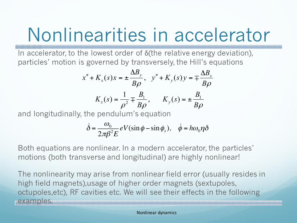
In accelerator, to the lowest order of δ(the relative energy deviation), particles’ motion is governed by transversely, the Hill’s equations

and longitudinally, the pendulum’s equation

Both equations are nonlinear. In a modern accelerator, the particles’ motions (both transverse and longitudinal) are highly nonlinear!

The nonlinearity may arise from nonlinear field error (usually resides in high field magnets),usage of higher order magnets (sextupoles, octupoles,etc), RF cavities etc. We will see their effects in the following examples.

Nonlineardynamics

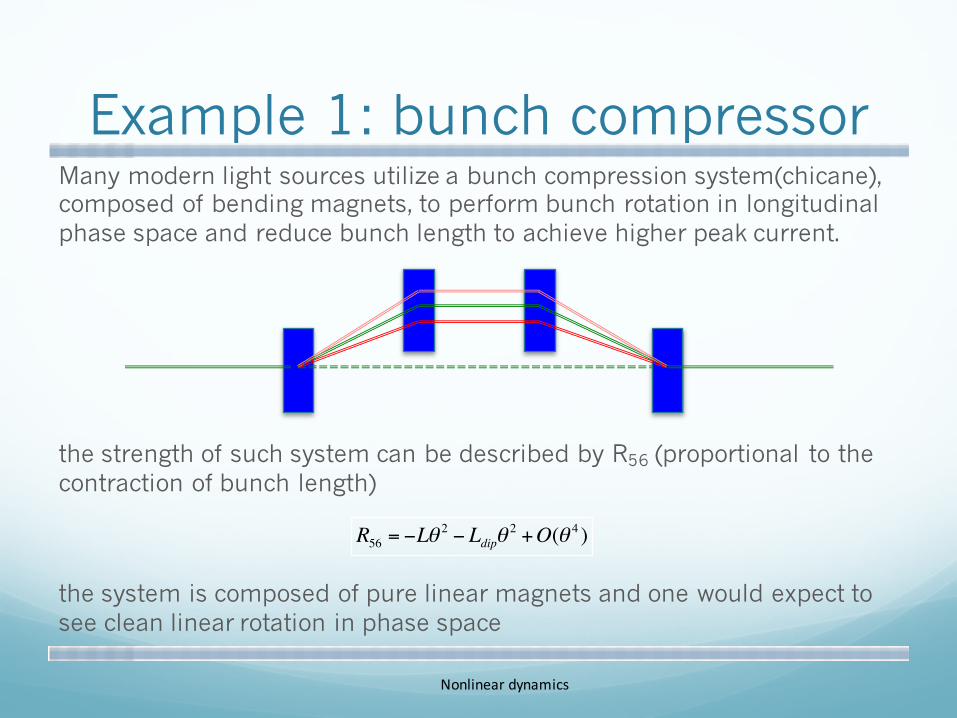
Example 1: bunch compressorMany modern light sources utilize a bunch compression system(chicane), composed of bending magnets, to perform bunch rotation in longitudinal phase space and reduce bunch length to achieve higher peak current.

the strength of such system can be described by R56 (proportional to the contraction of bunch length)

the system is composed of pure linear magnets and one would expect to see clean linear rotation in phase space

R56 = −Lθ2 − Ldipθ

2 +O(θ 4 )

Nonlineardynamics

Example 1: bunch compressor

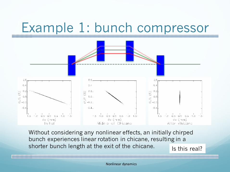
Without considering any nonlinear effects, an initially chirped bunch experiences linear rotation in chicane, resulting in a shorter bunch length at the exit of the chicane. Is this real?

Nonlineardynamics

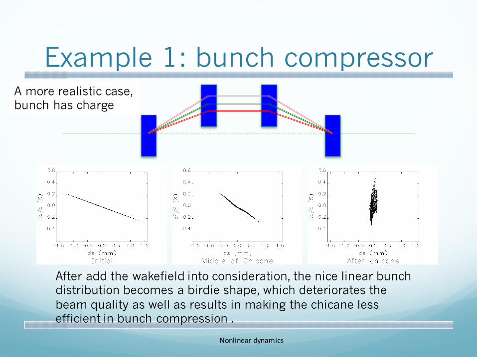
Example 1: bunch compressorA more realistic case, bunch has charge

After add the wakefield into consideration, the nice linear bunch distribution becomes a birdie shape, which deteriorates the beam quality as well as results in making the chicane less efficient in bunch compression .

Nonlineardynamics

Example 2: storage ring

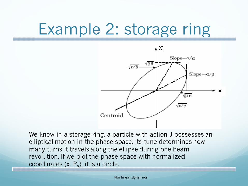
We know in a storage ring, a particle with action J possesses an elliptical motion in the phase space. Its tune determines how many turns it travels along the ellipse during one beam revolution. If we plot the phase space with normalized coordinates (x, Px), it is a circle.

X’

X

Nonlineardynamics

Example 2: storage ring

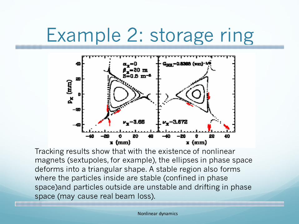
Tracking results show that with the existence of nonlinear magnets (sextupoles, for example), the ellipses in phase space deforms into a triangular shape. A stable region also forms where the particles inside are stable (confined in phase space)and particles outside are unstable and drifting in phase space (may cause real beam loss).

Nonlineardynamics

Nonlinearities in accelerator can’t be avoided

From above examples, we can see:

① Nonlinear effects are important in many diverse accelerator systems, and can arise even in systems comprising elements that are often considered “linear”.

② Nonlinear effects can occur in the longitudinal or transverse motion of particles moving along an accelerator beam line.

③ To understand nonlinear dynamics in accelerators we need to be able to construct dynamical maps for individual elements and complete systems and analyze these maps to understand the impact of nonlinearities on the performance of the system.

① If we have an accurate and thorough understanding of nonlinear dynamics in accelerators, we can attempt to mitigate adverse effects from nonlinearities.

Nonlineardynamics

Canonical transformationCanonical transformation is a transformation from a set of canonical variables to another. For example, the new set of variables X is transformed by an existing set of canonical variables x by:

the new set of variables obeys Hamilton’s equations

and we call X canonical variables. Please note that from the definition of canonical transformation, it is naturally symplectic.

In accelerator physics, it is often convenient to transform the cartesiancoordinates (x, px, y, py) into the action-angle variables (J, Φ).

∂X∂x

= A, and AT JA = JX = X(x)

X = J ∂H∂X

Nonlineardynamics

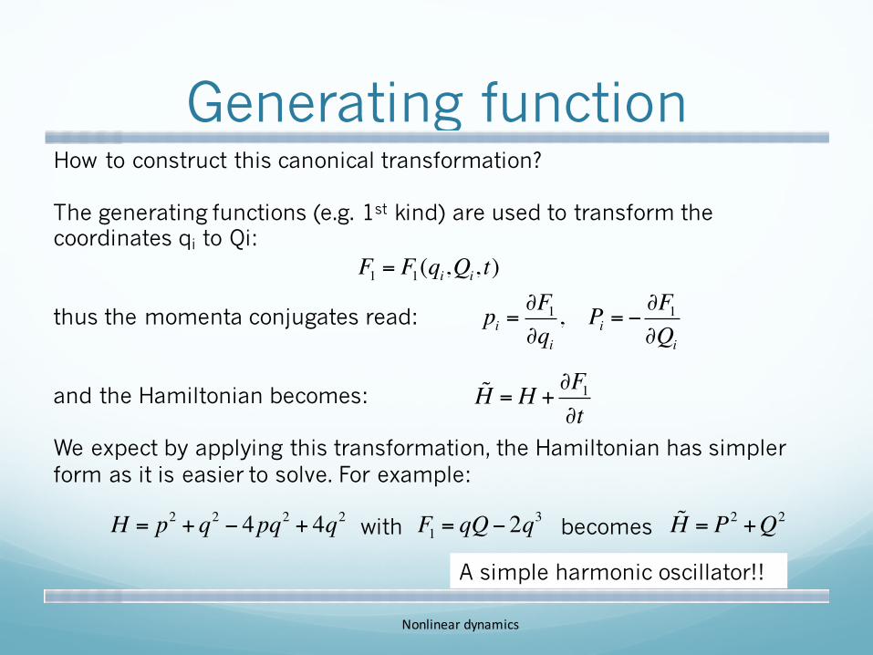
Generating functionHow to construct this canonical transformation?

The generating functions (e.g. 1st kind) are used to transform the coordinates qi to Qi:

thus the momenta conjugates read:

and the Hamiltonian becomes:

We expect by applying this transformation, the Hamiltonian has simpler form as it is easier to solve. For example:

with becomes

F1 = F1(qi,Qi, t)

pi =∂F1∂qi, Pi = −

∂F1∂Qi

H = H +∂F1∂t

H = p2 + q2 − 4pq2 + 4q2 F1 = qQ− 2q3 H = P2 +Q2

A simple harmonic oscillator!!

Nonlineardynamics

Action-angle variablesThe action angle variable (J, Φ) is defined as:

where (α,β,γ) are Twiss parameters. The action angle variable is very important for linear beam dynamics. As we all know, for linear dynamics, it has properties

using a generating function

and the Hamiltonian reduces to note this H is s dependent!

2Jz = γ zz2 + 2αzzz '+βzz '

2,

tanφz = −αz −βzz 'z

dJzds

= 0, dφzs=1βz

H =Jzβz

F1(z,φz ) = −z2

2βz(tanφx +αx )

Nonlineardynamics

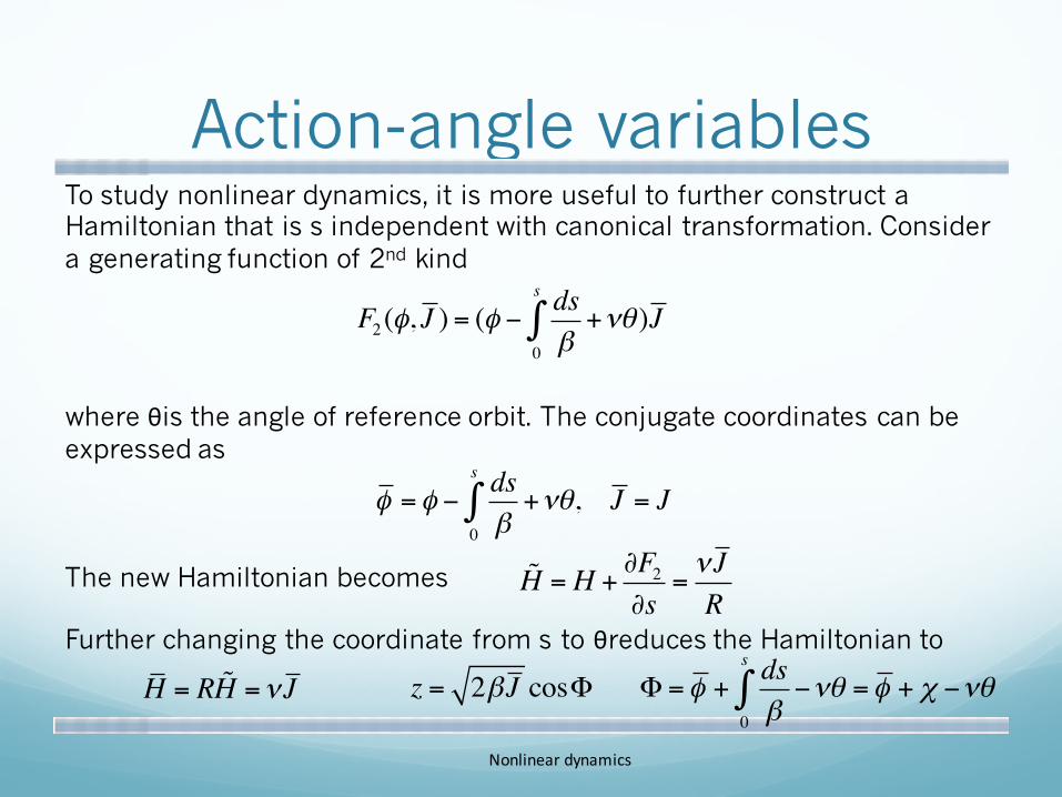
Action-angle variablesTo study nonlinear dynamics, it is more useful to further construct a Hamiltonian that is s independent with canonical transformation. Consider a generating function of 2nd kind

where θis the angle of reference orbit. The conjugate coordinates can be expressed as

The new Hamiltonian becomes

Further changing the coordinate from s to θreduces the Hamiltonian to

F2 (φ, J ) = (φ −dsβ+νθ

0

s

∫ )J

H = H +∂F2∂s

=νJR

φ = φ −dsβ+νθ

0

s

∫ , J = J

H = R H =νJ z = 2βJ cosΦ Φ = φ +dsβ−νθ

0

s

∫ = φ + χ −νθ

Nonlineardynamics

Treatments of nonlinearitiesA number of powerful tools for analysis of nonlinear systems can be developed from Hamiltonian mechanics to describe the motion for a particle moving through a component in an accelerator beamline:(truncated) power series; Lie transform; (implicit) generating function.

Hamiltonian is usually not integrable. However, if the Hamiltonian can be written as a sum of integrable terms, an explicit symplectic integrator that is accurate to some specified order can be constructed to solve the system.

For a storage ring, We mainly discuss two approaches to analyze nonlinear dynamics:1. Canonical perturbation method where nonlinear terms are treated as

perturbation to the linear Hamiltonian (may not give correct pictures when nonlinear magnets are strong)

2. Normal form analysis, based on Lie transformation of the one-turn map (especially useful when dealing with resonance driving terms and dynamic aperture problems) Nonlineardynamics

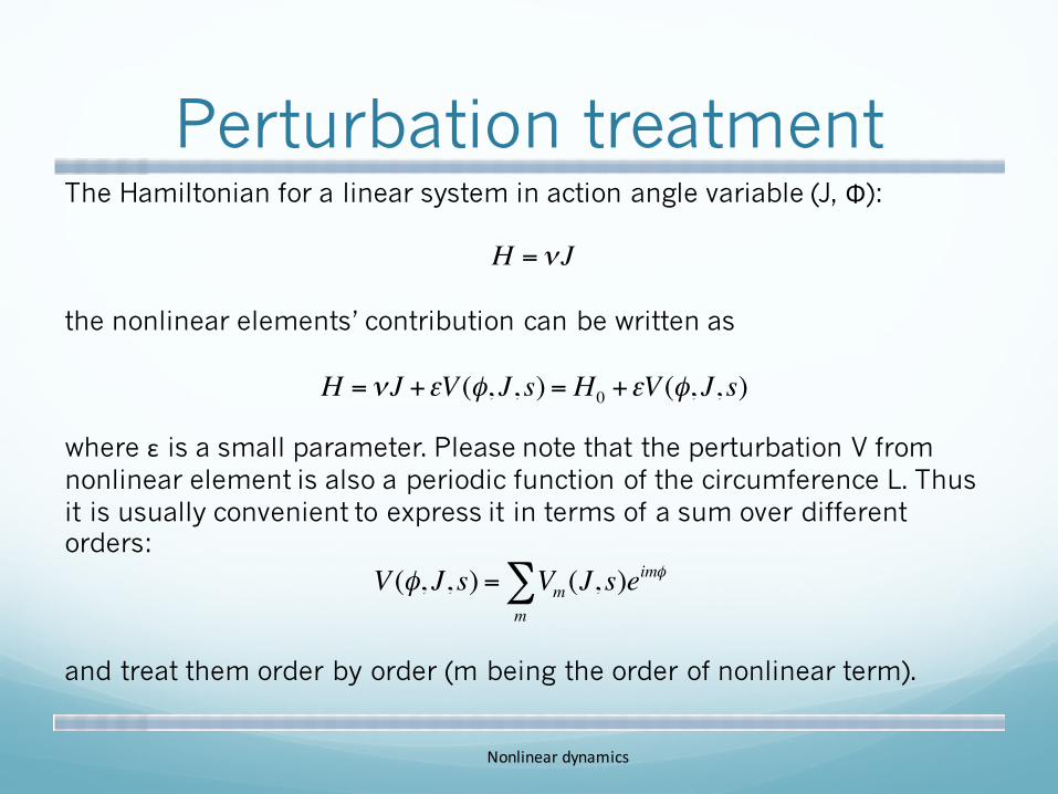
Perturbation treatmentThe Hamiltonian for a linear system in action angle variable (J, Φ):

the nonlinear elements’ contribution can be written as

where ε is a small parameter. Please note that the perturbation V from nonlinear element is also a periodic function of the circumference L. Thus it is usually convenient to express it in terms of a sum over different orders:

and treat them order by order (m being the order of nonlinear term).

V (φ, J, s) = Vm (J, s)eimφ

m∑

H =νJ

H =νJ +εV (φ, J, s) = H0 +εV (φ, J, s)

Nonlineardynamics

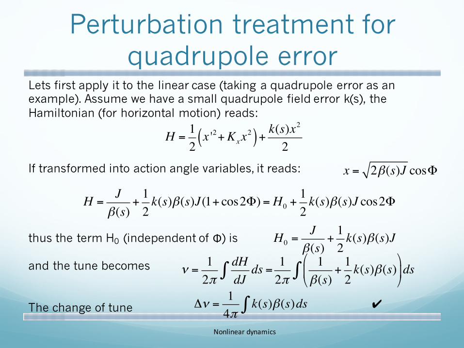
Perturbation treatment for quadrupole error

Lets first apply it to the linear case (taking a quadrupole error as an example). Assume we have a small quadrupole field error k(s), the Hamiltonian (for horizontal motion) reads:

If transformed into action angle variables, it reads:

thus the term H0 (independent of Φ) is

and the tune becomes

The change of tune

H =12x '2+Kxx

2( )+ k(s)x2

2

H =J

β(s)+12k(s)β(s)J(1+ cos2Φ) = H0 +

12k(s)β(s)J cos2Φ

x = 2β(s)J cosΦ

H0 =J

β(s)+12k(s)β(s)J

ν =12π

dHdJ

ds =∫ 12π

1β(s)

+12k(s)β(s)

"

#$

%

&'ds∫

Δν =14π

k(s)β(s)ds∫ ✔

Nonlineardynamics

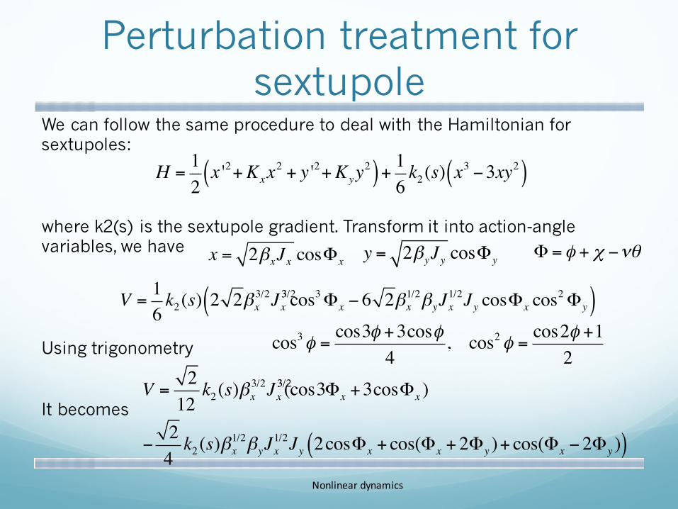
Perturbation treatment for sextupole

We can follow the same procedure to deal with the Hamiltonian for sextupoles:

where k2(s) is the sextupole gradient. Transform it into action-angle variables, we have

Using trigonometry

It becomes

H =12x '2+Kxx

2 + y '2+Kyy2( )+ 16 k2 (s) x

3 −3xy2( )

x = 2βxJx cosΦx y = 2βyJy cosΦy

V =16k2 (s) 2 2βx

3/2Jx3/23 cos3Φx − 6 2βx

1/2βyJx1/2Jy cosΦx cos

2Φy( )cos3φ = cos3φ +3cosφ

4, cos2φ = cos2φ +1

2

V =212

k2 (s)βx3/2Jx

3/23(cos3Φx +3cosΦx )

−24k2 (s)βx

1/2βyJx1/2Jy 2cosΦx + cos(Φx + 2Φy )+ cos(Φx − 2Φy )( )

Φ = φ + χ −νθ

Nonlineardynamics

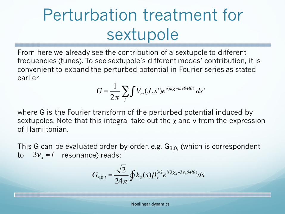
Perturbation treatment for sextupole

From here we already see the contribution of a sextupole to different frequencies (tunes). To see sextupole’s different modes’ contribution, it is convenient to expand the perturbed potential in Fourier series as stated earlier

where G is the Fourier transform of the perturbed potential induced by sextupoles. Note that this integral take out the χ and ν from the expression of Hamiltonian.

This G can be evaluated order by order, e.g. G3,0,l (which is correspondent to resonance) reads:

G =12π

Vm (J, s ')ei(mχ−mνθ+lθ ) ds '∫

l∑

G3,0,l =2

24πk2 (s)βx

3/2ei(3χ x−3ν xθ+lθ )∫ ds

3ν x = l

Nonlineardynamics

Perturbation treatment for sextupole

The Hamiltonian (in orbit angle θ) can be written as

where G’s drive the correspondent resonances and … drives parametric resonance

H =ν xJx +ν yJy + G3,0,l Jx3/2 cos(3φx − lθ )

l∑

+ G1,2,l Jx1/2Jy cos(φx + 2φy − lθ )+

l∑ G1,−2,l JxJy

1/2 cos(φx − 2φy − lθ )l∑ +…

ν x = l

Nonlineardynamics

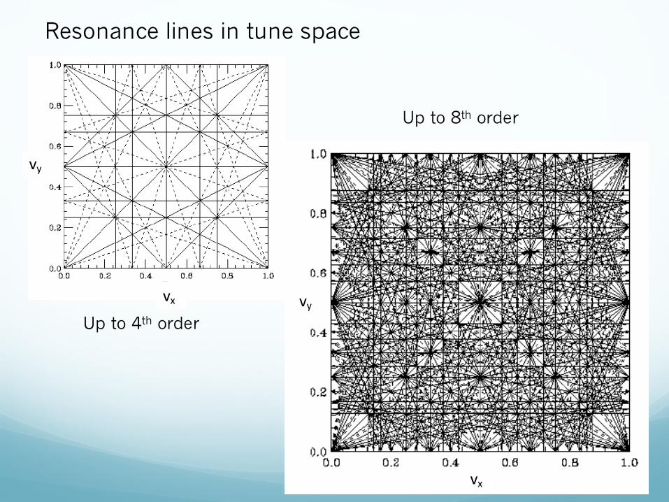
Resonance lines in tune space

vx

vy

vx

vyUp to 4th order

Up to 8th order

Nonlineardynamics

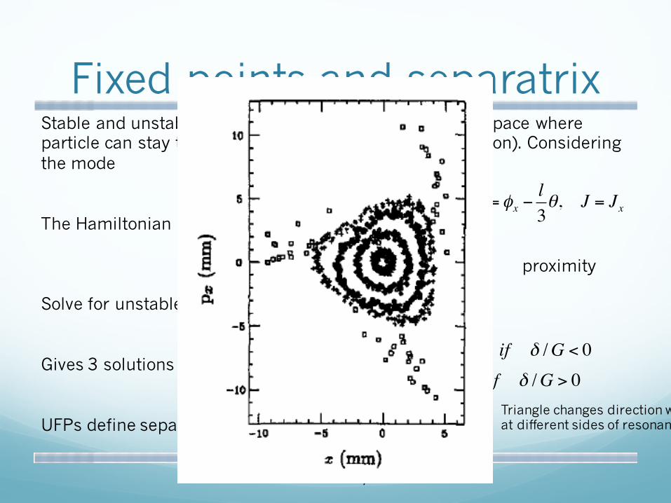
Fixed points and separatrixStable and unstable fixed points are the points in phase space where particle can stay there indefinitely (without any perturbation). Considering the mode , with generating function

The Hamiltonian becomes

Solve for unstable fixed points

Gives 3 solutions

UFPs define separatrix (the boundary of stable region)

3ν x = l

F2 = (φx −l3θ )J φ = φx −

l3θ, J = Jx

H = δJ +G3,0,l J3/2 cos3φ, δ =ν x −

l3

dJdθ

=dφdθ

= 0

proximity

JUFP1/2 =

2δ3G

φUFP = 0,±2π / 3, if δ /G < 0φUFP = ±π / 3,π if δ /G > 0

Triangle changes direction when at different sides of resonance

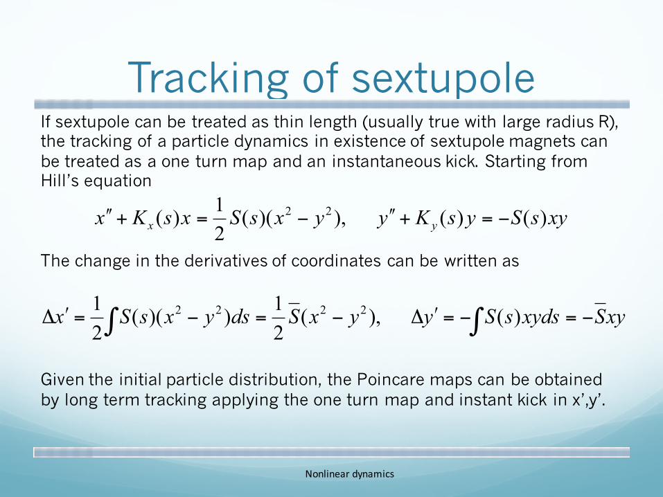
Tracking of sextupoleIf sextupole can be treated as thin length (usually true with large radius R), the tracking of a particle dynamics in existence of sextupole magnets can be treated as a one turn map and an instantaneous kick. Starting from Hill’s equation

The change in the derivatives of coordinates can be written as

Given the initial particle distribution, the Poincare maps can be obtained by long term tracking applying the one turn map and instant kick in x’,y’.

xysSysKyyxsSxsKx yx )()( ),)((21)( 22 −=+ʹ́−=+ʹ́

∫∫ −=−=ʹΔ−=−=ʹΔ xySxydssSyyxSdsyxsSx )( ,)(21))((

21 2222

Nonlineardynamics

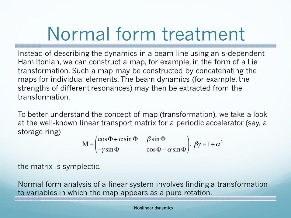
Normal form treatmentInstead of describing the dynamics in a beam line using an s-dependent Hamiltonian, we can construct a map, for example, in the form of a Lie transformation. Such a map may be constructed by concatenating the maps for individual elements. The beam dynamics (for example, the strengths of different resonances) may then be extracted from the transformation.

To better understand the concept of map (transformation), we take a look at the well-known linear transport matrix for a periodic accelerator (say, a storage ring)

the matrix is symplectic.

Normal form analysis of a linear system involves finding a transformation to variables in which the map appears as a pure rotation.

M =cosΦ+α sinΦ−γ sinΦ#

$%

β sinΦcosΦ−α sinΦ

&

'(, βγ =1+α 2

Nonlineardynamics

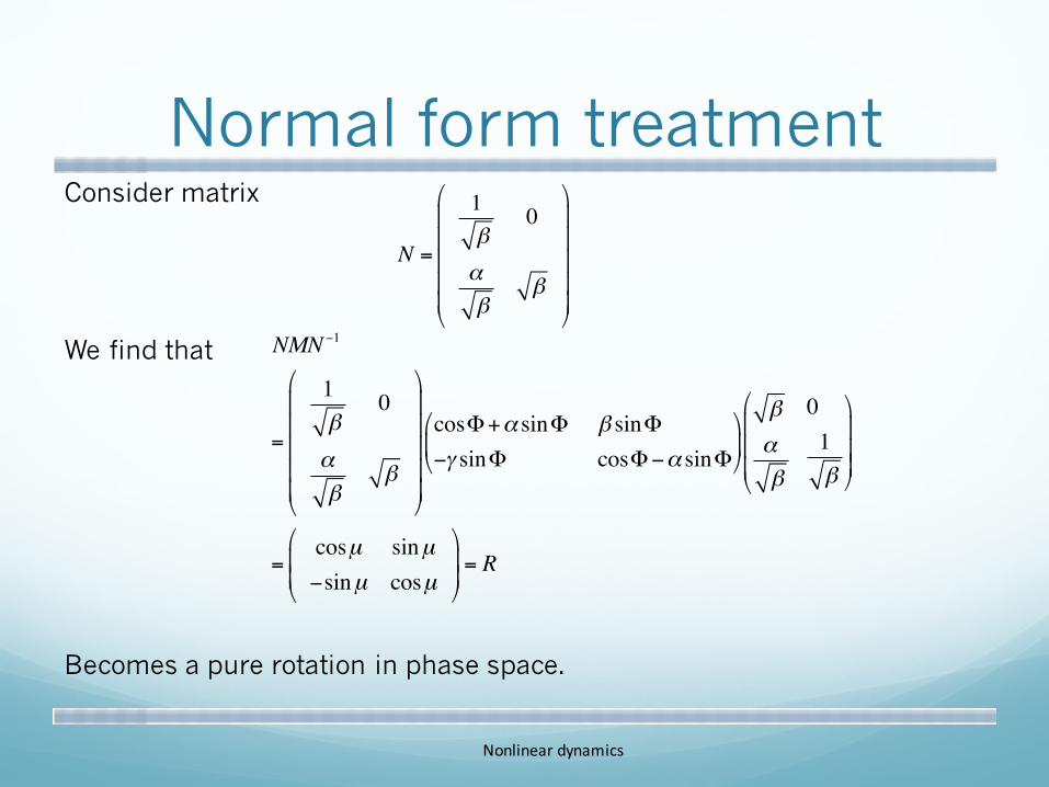
Normal form treatmentConsider matrix

We find that

Becomes a pure rotation in phase space.

N =

1β

0

αβ

β

!

"

#####

$

%

&&&&&

NMN −1

=

1β

0

αβ

β

"

#

$$$$$

%

&

'''''

cosΦ+α sinΦ−γ sinΦ"

#$

β sinΦcosΦ−α sinΦ

%

&'

β

αβ

"

#

$$$

0

1β

%

&

'''

=cosµ sinµ−sinµ cosµ

"

#$$

%

&''= R

Nonlineardynamics

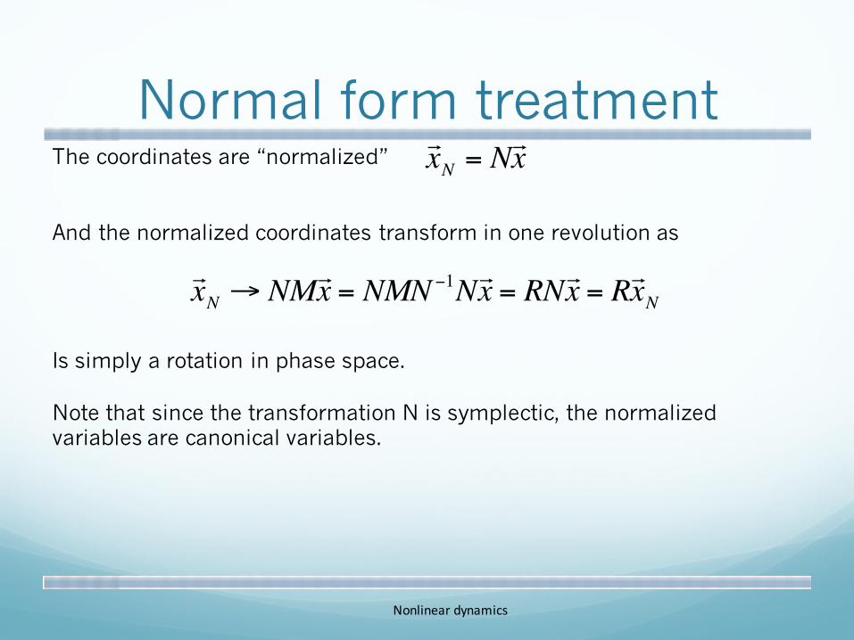
Normal form treatmentThe coordinates are “normalized”

And the normalized coordinates transform in one revolution as

Is simply a rotation in phase space.

Note that since the transformation N is symplectic, the normalized variables are canonical variables.

xN = Nx

xN → NMx = NMN −1Nx = RNx = RxN

Nonlineardynamics

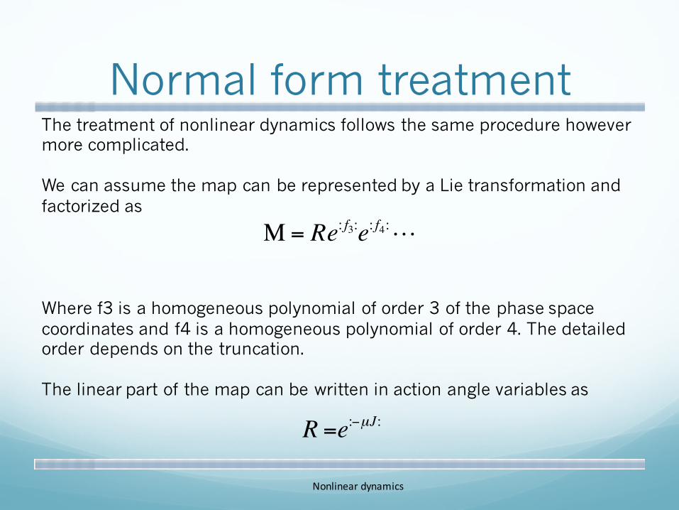
Normal form treatmentThe treatment of nonlinear dynamics follows the same procedure however more complicated.

We can assume the map can be represented by a Lie transformation and factorized as

Where f3 is a homogeneous polynomial of order 3 of the phase space coordinates and f4 is a homogeneous polynomial of order 4. The detailed order depends on the truncation.

The linear part of the map can be written in action angle variables as

Μ = Re: f3:e: f4:

R =e:−µJ:

Nonlineardynamics

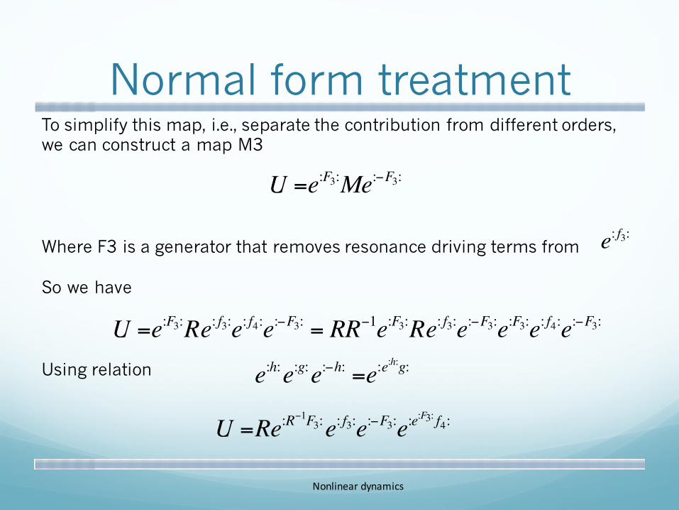
Normal form treatmentTo simplify this map, i.e., separate the contribution from different orders, we can construct a map M3

Where F3 is a generator that removes resonance driving terms from

So we have

Using relation

U =e:F3:Me:−F3:

e:h:e:g:e:−h: =e:e:h:g:

e: f3:

U =e:F3:Re: f3:e: f4:e:−F3: = RR−1e:F3:Re: f3:e:−F3:e:F3:e: f4:e:−F3:

U =Re:R−1F3:e: f3:e:−F3:e:e

:F3: f4:

Nonlineardynamics

Normal form treatmentUsing Baker-Campbell-Hausdorff formula

The map now becomes

We can further reduce it to (non-trivial)

Where contains all the 3rd order contribution.

e:A:e:B: = e:C:, where C = A+B+ 12[A,B]+

U =Re:R−1F3+ f3−F3+O(4):e:e

:F3: f4:

U =Re: f3(1):e: f4

(1): = Re:R−1F3+ f3−F3:e: f4

(1):

f3(1) = R−1F3 + f3 −F3

Nonlineardynamics

Normal form treatmentThus the solution is

Since f3 is periodic in the angle variable Φ, we can write

We can construct a f3(1) that does not have phase dependence, i.e., we can write it as

Thus now the generation function F3 reads

F3 =f3 − f3

(1)

I − R−1

f3 = f3,m (J )eimφ

m∑

f (1)3 = f3,0 (J )

F3 =f3,m (J )e

imφ

1− e−imµm≠0∑

Nonlineardynamics

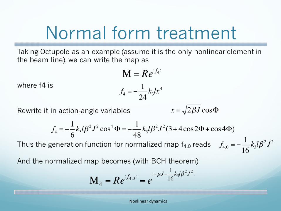
Normal form treatmentTaking Octupole as an example (assume it is the only nonlinear element in the beam line), we can write the map as

where f4 is

Rewrite it in action-angle variables

Thus the generation function for normalized map f4,0 reads

And the normalized map becomes (with BCH theorem)

f4 = −124k3lx

4

Nonlineardynamics

Μ = Re: f4:

f4 = −16k3lβ

2J 2 cos4Φ = −148k3lβ

2J 2 (3+ 4cos2Φ+ cos4Φ)

x = 2βJ cosΦ

f4,0 = −116k3lβ

2J 2

Μ4 = Re: f4,0: = e

:−µJ− 116k3lβ

2J 2:

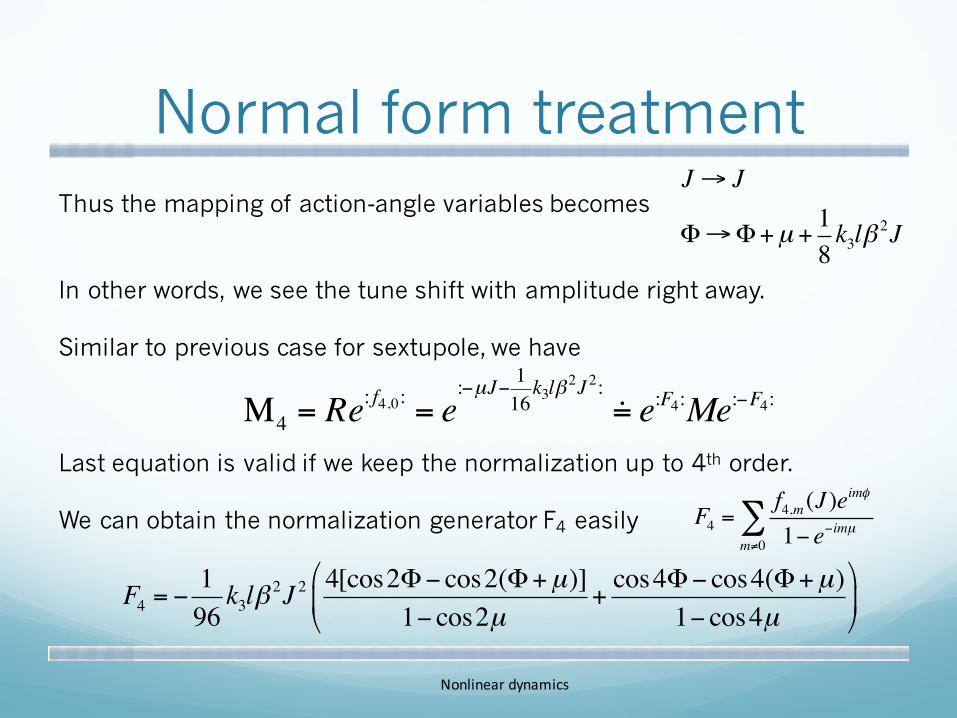
Normal form treatmentThus the mapping of action-angle variables becomes

In other words, we see the tune shift with amplitude right away.

Similar to previous case for sextupole, we have

Last equation is valid if we keep the normalization up to 4th order.

We can obtain the normalization generator F4 easily

Nonlineardynamics

J→ J

Φ→Φ+µ +18k3lβ

2J

Μ4 = Re: f4,0: = e

:−µJ− 116k3lβ

2J 2:= e:F4:Me:−F4:

F4 = −196k3lβ

2J 2 4[cos2Φ− cos2(Φ+µ)]1− cos2µ

+cos4Φ− cos4(Φ+µ)

1− cos4µ#

$%

&

'(

F4 =f4,m (J )e

imφ

1− e−imµm≠0∑

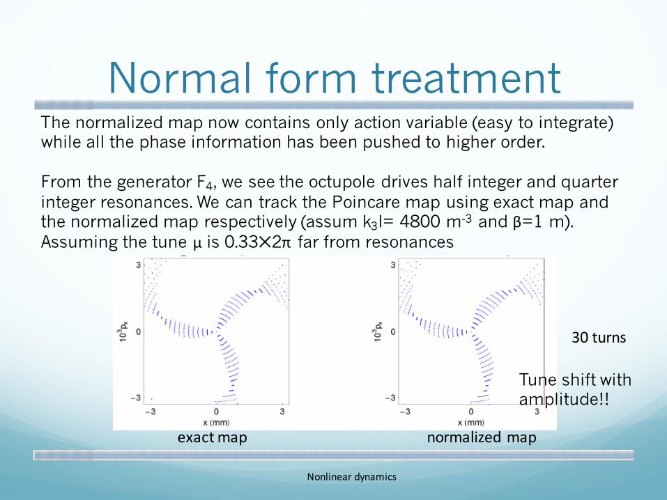
Normal form treatmentThe normalized map now contains only action variable (easy to integrate) while all the phase information has been pushed to higher order.

From the generator F4, we see the octupole drives half integer and quarter integer resonances. We can track the Poincare map using exact map and the normalized map respectively (assum k3l= 4800 m-3 and β=1 m). Assuming the tune μ is 0.33✕2π far from resonances

Nonlineardynamics

exactmapnormalizedmap

30turns

Tune shift with amplitude!!

Normal form treatment

Nonlineardynamics

exactmapnormalizedmap

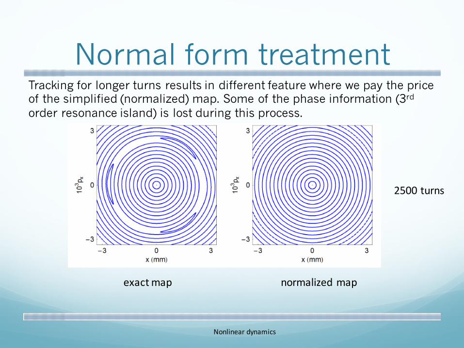
2500turns

Tracking for longer turns results in different feature where we pay the price of the simplified (normalized) map. Some of the phase information (3rd

order resonance island) is lost during this process.

Normal form treatment

Nonlineardynamics

exactmapnormalizedmap

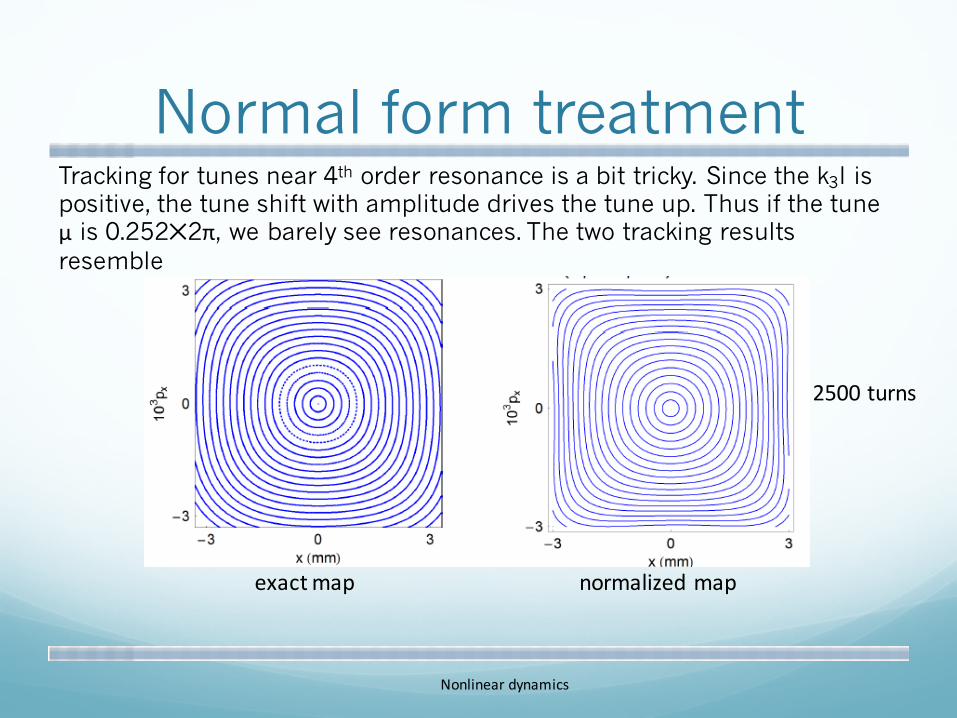
2500turns

Tracking for tunes near 4th order resonance is a bit tricky. Since the k3l is positive, the tune shift with amplitude drives the tune up. Thus if the tune μ is 0.252✕2π, we barely see resonances. The two tracking results resemble

Normal form treatment

Nonlineardynamics

exactmapnormalizedmap

2500turns

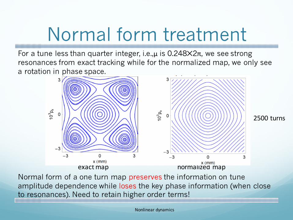
For a tune less than quarter integer, i.e.,μ is 0.248✕2π, we see strong resonances from exact tracking while for the normalized map, we only see a rotation in phase space.

Normal form of a one turn map preserves the information on tune amplitude dependence while loses the key phase information (when close to resonances). Need to retain higher order terms!

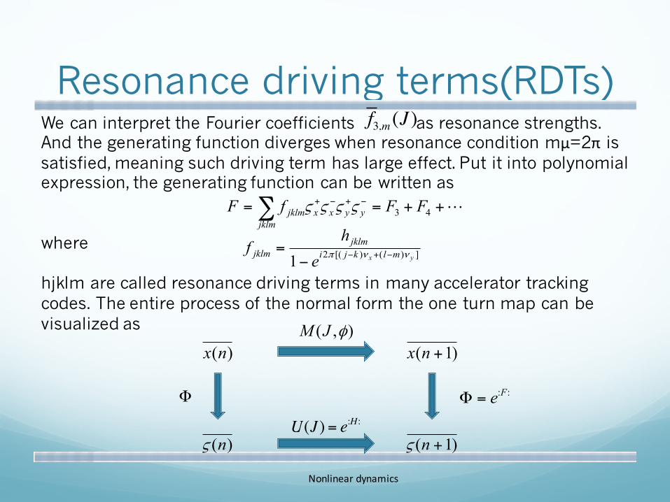
Resonance driving terms(RDTs)We can interpret the Fourier coefficients as resonance strengths. And the generating function diverges when resonance condition mμ=2π is satisfied, meaning such driving term has large effect. Put it into polynomial expression, the generating function can be written as

where

hjklm are called resonance driving terms in many accelerator tracking codes. The entire process of the normal form the one turn map can be visualized as

f3,m (J )

!++==∑ −+−+

jklmyyxxjklm FFfF 43ςςςς

])()[(21 yx mlkjijklm

jklm eh

f ννπ −+−−=

)(nx )1( +nx),( φJM

Φ ::Fe=Φ

)(nςU(J ) = e:H :

)1( +nς

Nonlineardynamics

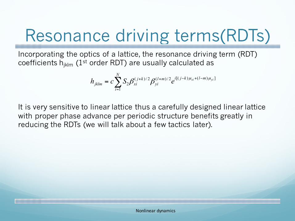
Resonance driving terms(RDTs)Incorporating the optics of a lattice, the resonance driving term (RDT) coefficients hjklm (1st order RDT) are usually calculated as

It is very sensitive to linear lattice thus a carefully designed linear lattice with proper phase advance per periodic structure benefits greatly in reducing the RDTs (we will talk about a few tactics later).

∑=

−+−++=N

i

mlkjimlyi

kjxijklm

yixieSch1

])()[(2/)(2/)(2

µµββ

Nonlineardynamics

Chromatic aberrationSextupoles (and even higher order magnets) are necessary in an accelerator design (not only existing as the field error of strong linear magnets).

Sextupoles are used to correct the chromatic aberration, i.e., tune shift, that resides in linear lattice (in comparison to the aberration that exists in optics).

We can define chromaticities

The chromaticity induced by quadrupole field is called natural chromaticity.

[ ][ ] δνδδβν

δνδδβν

π

π

ddCCdssKs

ddCCdssKs

yyyyyy

xxxxxx

/ ,)()(

/ ,)()(

41

41

=≡−=Δ

=≡−=Δ

∫∫

Nonlineardynamics

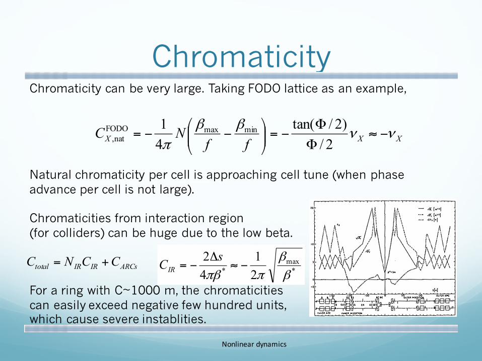
ChromaticityChromaticity can be very large. Taking FODO lattice as an example,

Natural chromaticity per cell is approaching cell tune (when phase advance per cell is not large).

Chromaticities from interaction region (for colliders) can be huge due to the low beta.

For a ring with C~1000 m, the chromaticitiescan easily exceed negative few hundred units, which cause severe instablities.

XXX ffNC νν

ββπ

−≈ΦΦ

−=⎟⎟⎠

⎞⎜⎜⎝

⎛−−=

2/)2/tan(

41 minmaxFODO

nat,

*max

* 21

42

ββ

ππβ−≈

Δ−=

sCIRARCsIRIRtotal CCNC +=

Nonlineardynamics

Chromaticity correction

Nonlineardynamics

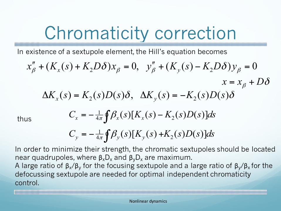
In existence of a sextupole element, the Hill’s equation becomes

thus

δβ Dxx +=

0))(( ,0))(( 22 =−+ʹ́=++ʹ́ ββββ δδ yDKsKyxDKsKx yx

δδ )()()( ,)()()( 22 sDsKsKsDsKsK yx −=Δ=Δ

dssDsKsKsC

dssDsKsKsC

yyy

xxx

)]()()()[(

)]()()()[(

241

241

∫∫

+−=

−−=

β

β

π

π

In order to minimize their strength, the chromatic sextupoles should be located near quadrupoles, where βxDx and βyDx are maximum.A large ratio of βx/βy for the focusing sextupole and a large ratio of βy/βx for the defocussing sextupole are needed for optimal independent chromaticity control.

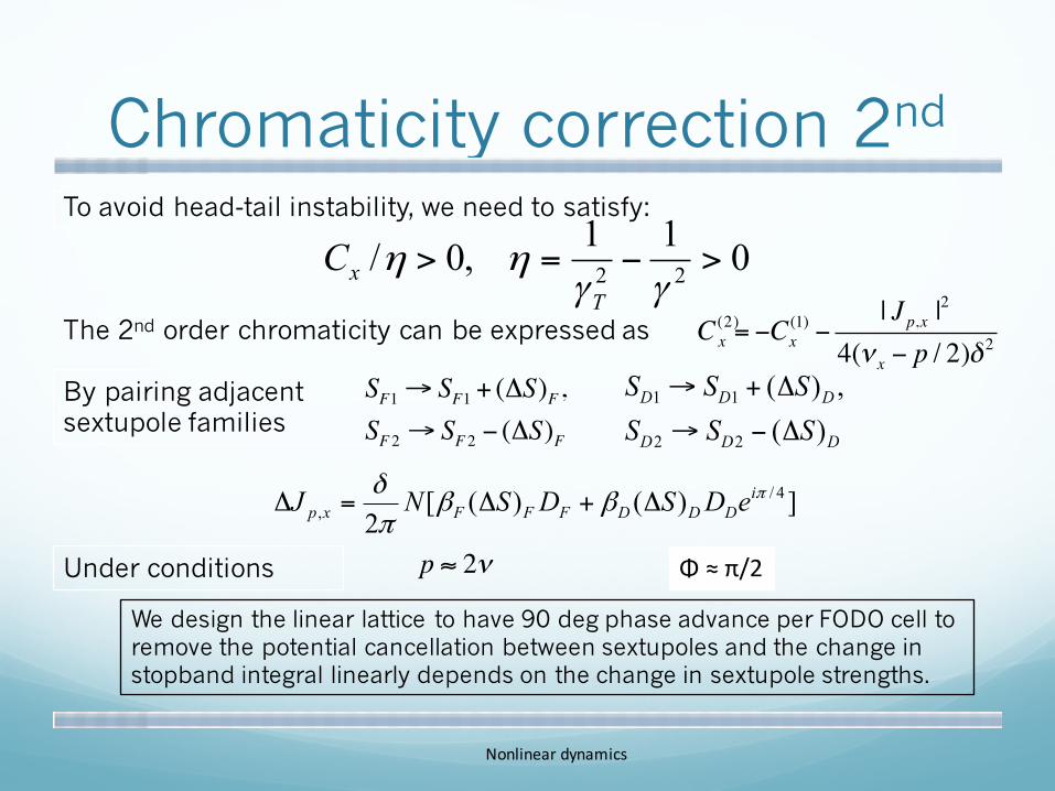
Chromaticity correction 2nd

Φ ≈π/2

C (2)x = −Cx

(1) −| Jp,x |

2

4(ν x − p / 2)δ2

By pairing adjacent sextupole families

SF1→ SF1 + (ΔS)F,SF2 → SF2 − (ΔS)F

Under conditions p ≈ 2ν

])()([2

4/,

πββπδ i

DDDFFFxp eDSDSNJ Δ+Δ=Δ

We design the linear lattice to have 90 deg phase advance per FODO cell to remove the potential cancellation between sextupoles and the change in stopband integral linearly depends on the change in sextupole strengths.

To avoid head-tail instability, we need to satisfy:

011,0/ 22 >−=>γγ

ηηT

xC

The 2nd order chromaticity can be expressed as

DDD

DDD

SSSSSS)(,)(

22

11

Δ−→

Δ+→

Nonlineardynamics

Dynamic aperture (DA)Dynamic aperture determines the stable region in 2d real space (x-y) while particles travel along the accelerator. It is very important for particle dynamic study especially in effects that requires tracking over many revolutions (decided by system’s damping time, could range from 1000 (light sources) to 1,000,000 (proton/heavy ion storage rings).

Dynamic aperture is a clear indication of nonlinear resonances that reside in an accelerator. Its size is limited by the utilize of nonlinear magnets to correct chromatic aberration. Thus designing the lattice with the nonlinear magnets’ strengths reduced is crucial in improving DA.

Careful tuning of multipole nonlinear elements can also result in reducing the resonance driving terms thus improving the DA.

There are many ways of determining the DA of a specific lattice. Mostly commonly used techniques include line search mode (single-line, n-line,etc…) and frequency map analysis.

Nonlineardynamics

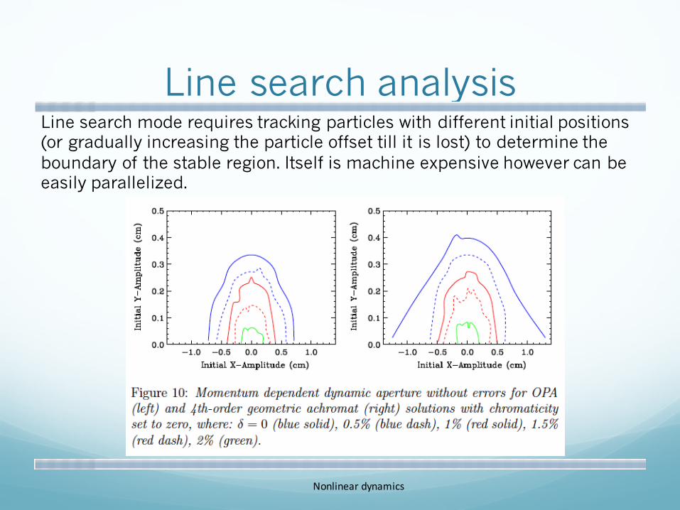
Line search analysisLine search mode requires tracking particles with different initial positions (or gradually increasing the particle offset till it is lost) to determine the boundary of the stable region. Itself is machine expensive however can be easily parallelized.

Nonlineardynamics

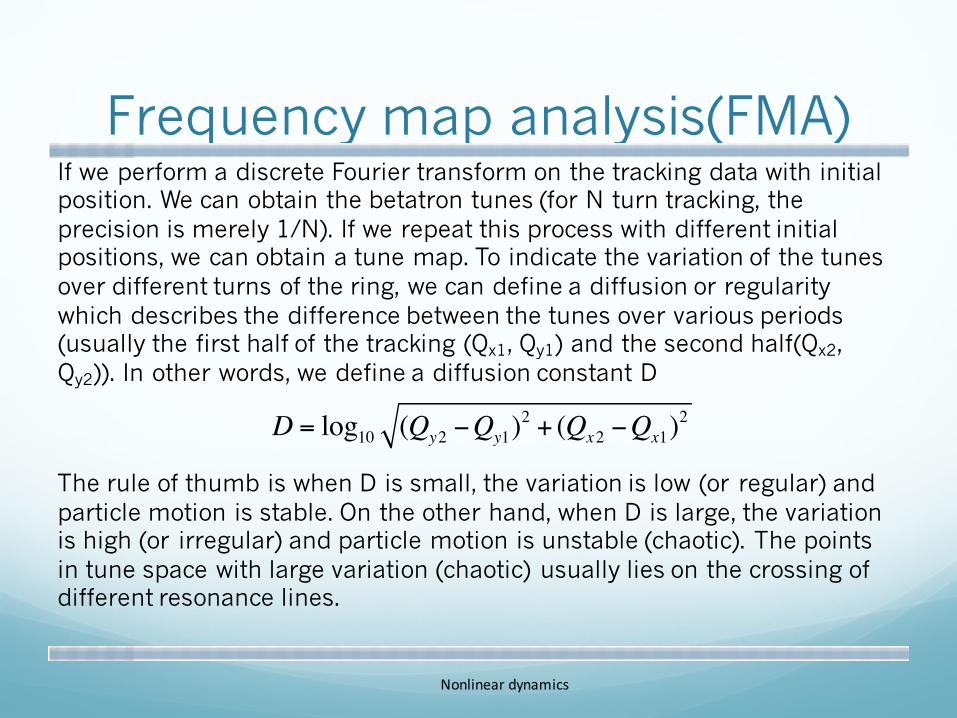
Frequency map analysis(FMA)If we perform a discrete Fourier transform on the tracking data with initial position. We can obtain the betatron tunes (for N turn tracking, the precision is merely 1/N). If we repeat this process with different initial positions, we can obtain a tune map. To indicate the variation of the tunes over different turns of the ring, we can define a diffusion or regularity which describes the difference between the tunes over various periods (usually the first half of the tracking (Qx1, Qy1) and the second half(Qx2, Qy2)). In other words, we define a diffusion constant D

The rule of thumb is when D is small, the variation is low (or regular) and particle motion is stable. On the other hand, when D is large, the variation is high (or irregular) and particle motion is unstable (chaotic). The points in tune space with large variation (chaotic) usually lies on the crossing of different resonance lines.

Nonlineardynamics

D = log10 (Qy2 −Qy1)2 + (Qx2 −Qx1)

2

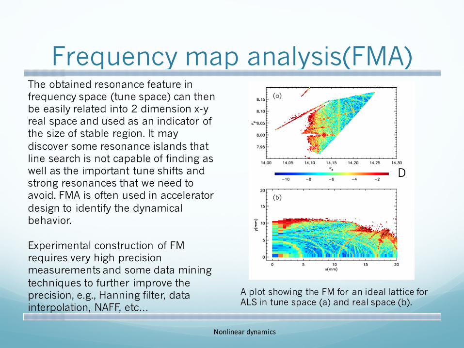
Frequency map analysis(FMA)The obtained resonance feature in frequency space (tune space) can then be easily related into 2 dimension x-y real space and used as an indicator of the size of stable region. It may discover some resonance islands that line search is not capable of finding as well as the important tune shifts and strong resonances that we need to avoid. FMA is often used in accelerator design to identify the dynamical behavior.

Experimental construction of FM requires very high precision measurements and some data mining techniques to further improve the precision, e.g., Hanning filter, data interpolation, NAFF, etc…

Nonlineardynamics

A plot showing the FM for an ideal lattice for ALS in tune space (a) and real space (b).

D