Nonlinear Algebraic Equations - Forside · Nonlinear algebraic equations Similarly, for any linear...
88
Nonlinear Algebraic Equations Lectures INF2320 – p. 1/88
Transcript of Nonlinear Algebraic Equations - Forside · Nonlinear algebraic equations Similarly, for any linear...

Nonlinear Algebraic Equations
Lectures INF2320 – p. 1/88
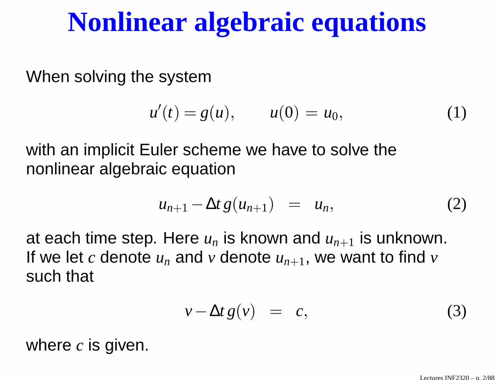
Nonlinear algebraic equations
When solving the system
u′(t) = g(u), u(0) = u0, (1)
with an implicit Euler scheme we have to solve thenonlinear algebraic equation
un+1−∆t g(un+1) = un, (2)
at each time step. Here un is known and un+1 is unknown.If we let c denote un and v denote un+1, we want to find vsuch that
v−∆t g(v) = c, (3)
where c is given.
Lectures INF2320 – p. 2/88
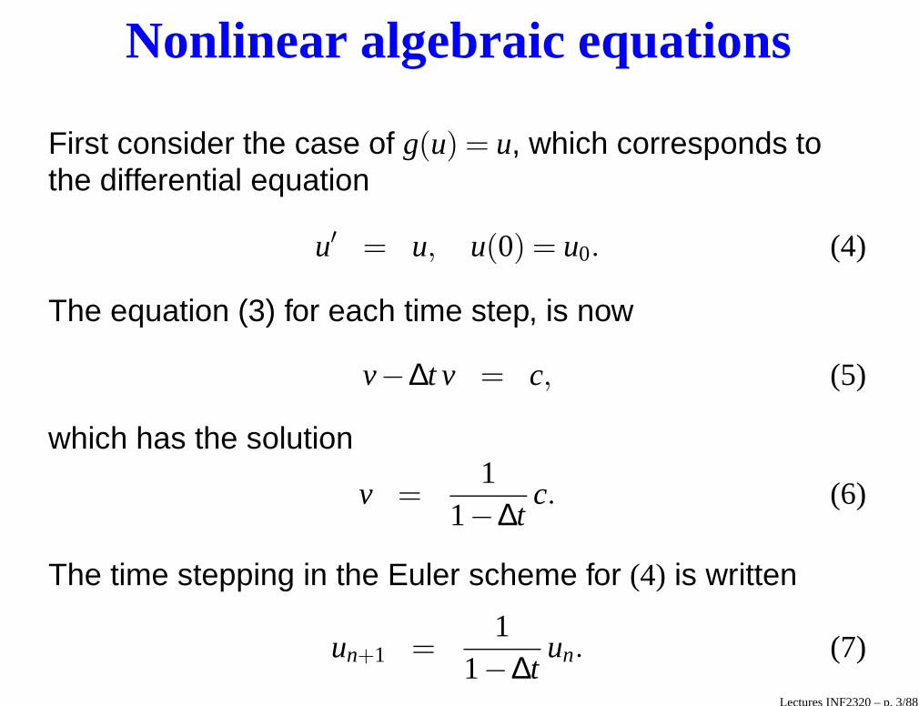
Nonlinear algebraic equations
First consider the case of g(u) = u, which corresponds tothe differential equation
u′ = u, u(0) = u0. (4)
The equation (3) for each time step, is now
v−∆t v = c, (5)
which has the solution
v =1
1−∆tc. (6)
The time stepping in the Euler scheme for (4) is written
un+1 =1
1−∆tun. (7)
Lectures INF2320 – p. 3/88
Nonlinear algebraic equations
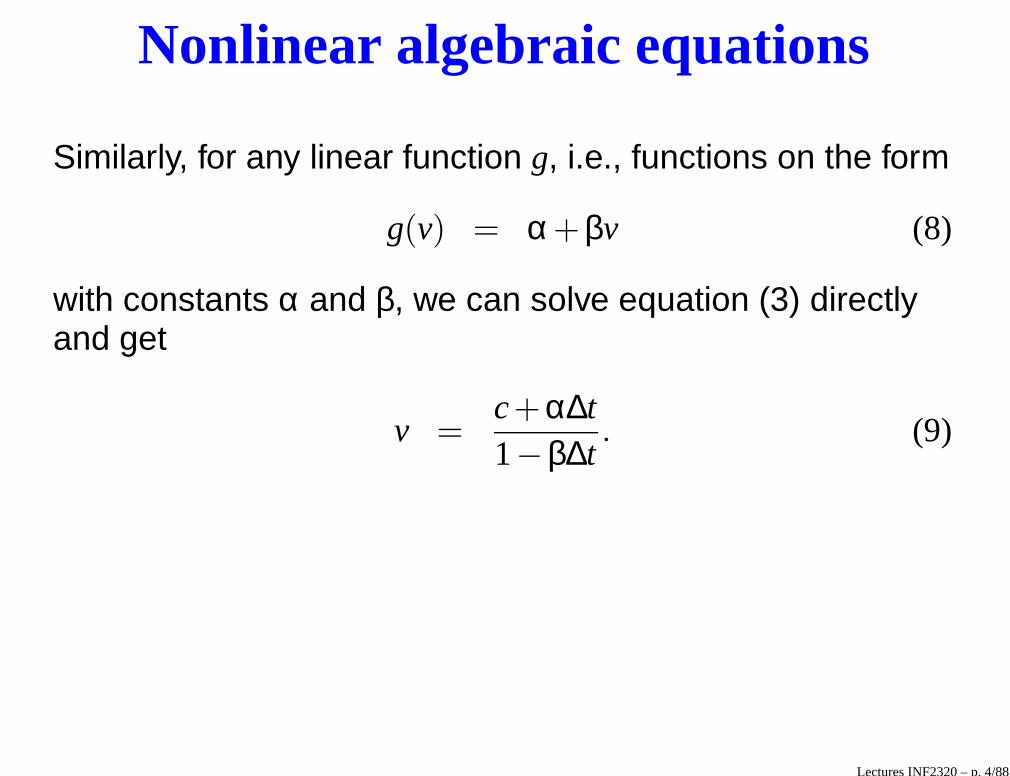
Similarly, for any linear function g, i.e., functions on the form
g(v) = α+βv (8)
with constants α and β, we can solve equation (3) directlyand get
v =c+α∆t1−β∆t
. (9)
Lectures INF2320 – p. 4/88
Nonlinear algebraic equations
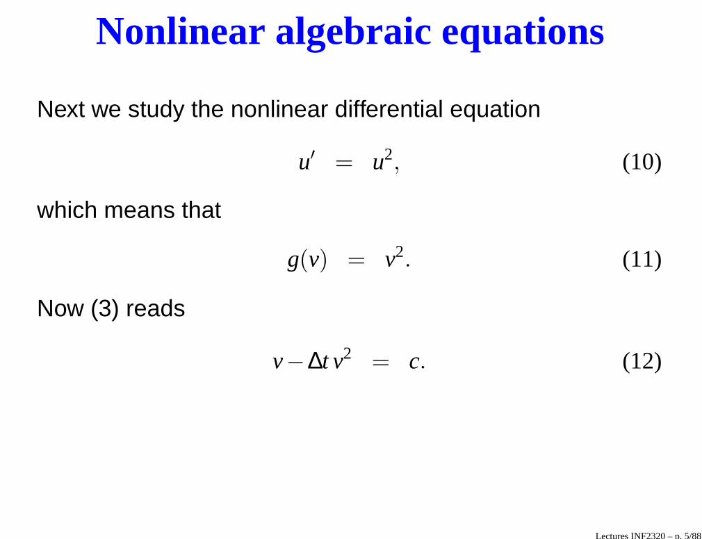
Next we study the nonlinear differential equation
u′ = u2, (10)
which means that
g(v) = v2. (11)
Now (3) reads
v−∆t v2 = c. (12)
Lectures INF2320 – p. 5/88
Nonlinear algebraic equations
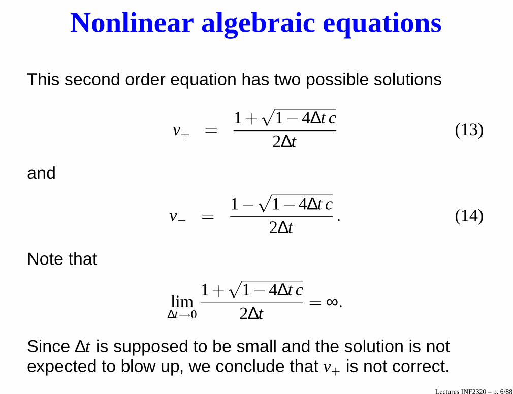
This second order equation has two possible solutions
v+ =1+
√1−4∆t c2∆t
(13)
and
v− =1−
√1−4∆t c2∆t
. (14)
Note that
lim∆t→0
1+√
1−4∆t c2∆t
= ∞.
Since ∆t is supposed to be small and the solution is notexpected to blow up, we conclude that v+ is not correct.
Lectures INF2320 – p. 6/88
Nonlinear algebraic equations
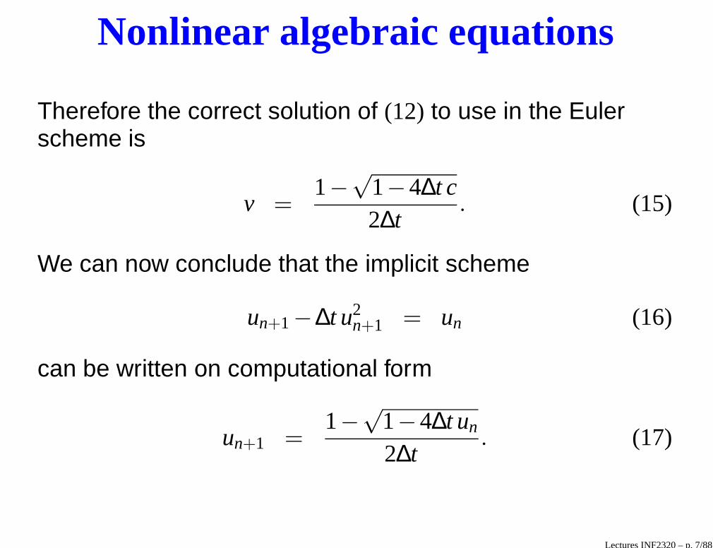
Therefore the correct solution of (12) to use in the Eulerscheme is
v =1−
√1−4∆t c2∆t
. (15)
We can now conclude that the implicit scheme
un+1−∆t u2n+1 = un (16)
can be written on computational form
un+1 =1−
√1−4∆t un
2∆t. (17)
Lectures INF2320 – p. 7/88
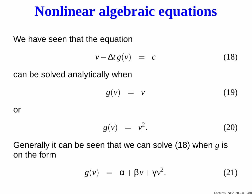
Nonlinear algebraic equations
We have seen that the equation
v−∆t g(v) = c (18)
can be solved analytically when
g(v) = v (19)
or
g(v) = v2. (20)
Generally it can be seen that we can solve (18) when g ison the form
g(v) = α+βv+ γv2. (21)
Lectures INF2320 – p. 8/88
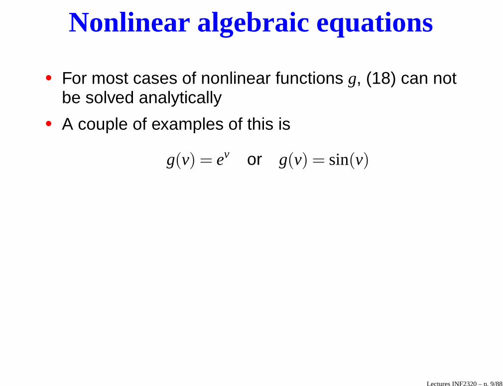
Nonlinear algebraic equations
• For most cases of nonlinear functions g, (18) can notbe solved analytically
• A couple of examples of this is
g(v) = ev or g(v) = sin(v)
Lectures INF2320 – p. 9/88
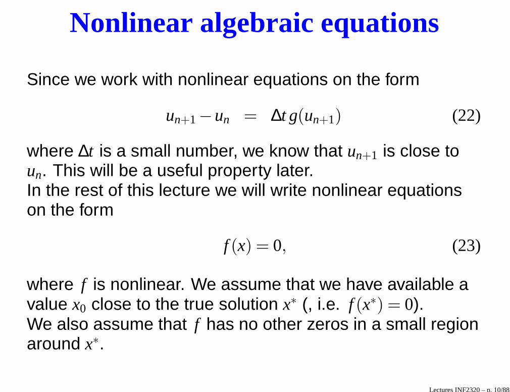
Nonlinear algebraic equations
Since we work with nonlinear equations on the form
un+1−un = ∆t g(un+1) (22)
where ∆t is a small number, we know that un+1 is close toun. This will be a useful property later.In the rest of this lecture we will write nonlinear equationson the form
f (x) = 0, (23)
where f is nonlinear. We assume that we have available avalue x0 close to the true solution x∗ (, i.e. f (x∗) = 0).We also assume that f has no other zeros in a small regionaround x∗.
Lectures INF2320 – p. 10/88
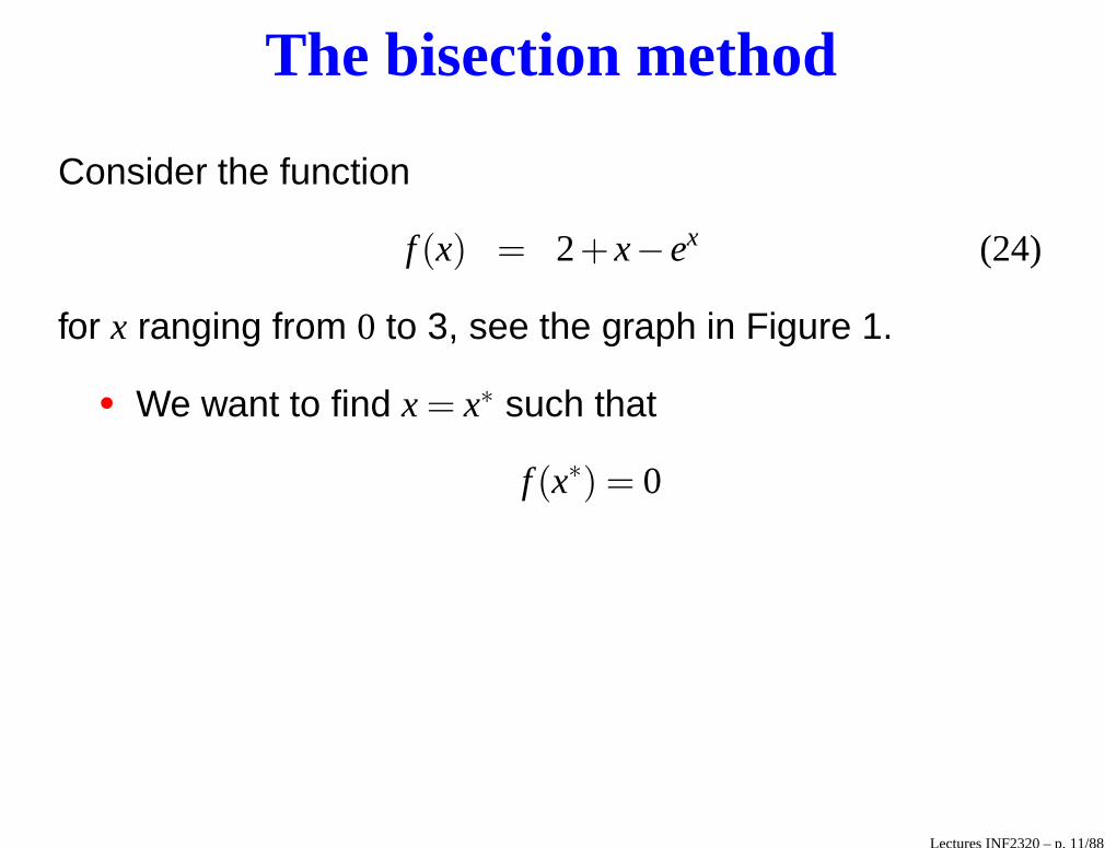
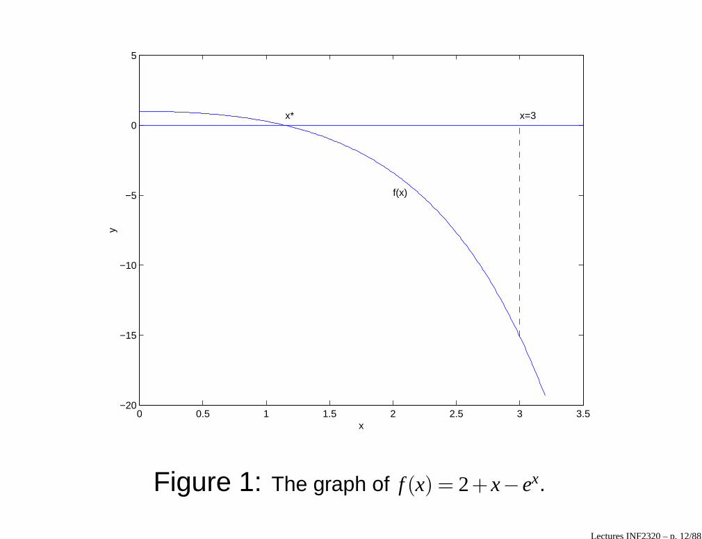
The bisection method
Consider the function
f (x) = 2+ x− ex (24)
for x ranging from 0 to 3, see the graph in Figure 1.
• We want to find x = x∗ such that
f (x∗) = 0
Lectures INF2320 – p. 11/88
0 0.5 1 1.5 2 2.5 3 3.5−20
−15
−10
−5
0
5
x* x=3
f(x)
x
y
Figure 1: The graph of f (x) = 2+ x− ex.
Lectures INF2320 – p. 12/88
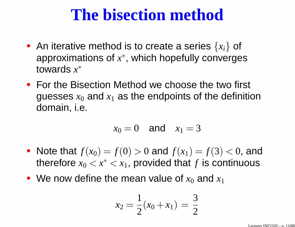
The bisection method
• An iterative method is to create a series {xi} ofapproximations of x∗, which hopefully convergestowards x∗
• For the Bisection Method we choose the two firstguesses x0 and x1 as the endpoints of the definitiondomain, i.e.
x0 = 0 and x1 = 3
• Note that f (x0) = f (0) > 0 and f (x1) = f (3) < 0, andtherefore x0 < x∗ < x1, provided that f is continuous
• We now define the mean value of x0 and x1
x2 =12(x0 + x1) =
32
Lectures INF2320 – p. 13/88
0 0.5 1 1.5 2 2.5 3 3.5−20
−15
−10
−5
0
5
x1=3
x0=0
x2=1.5
x
y
Figure 2: The graph of f (x) = 2+ x− ex and three values of f :
f (x0), f (x1) and f (x2).
Lectures INF2320 – p. 14/88
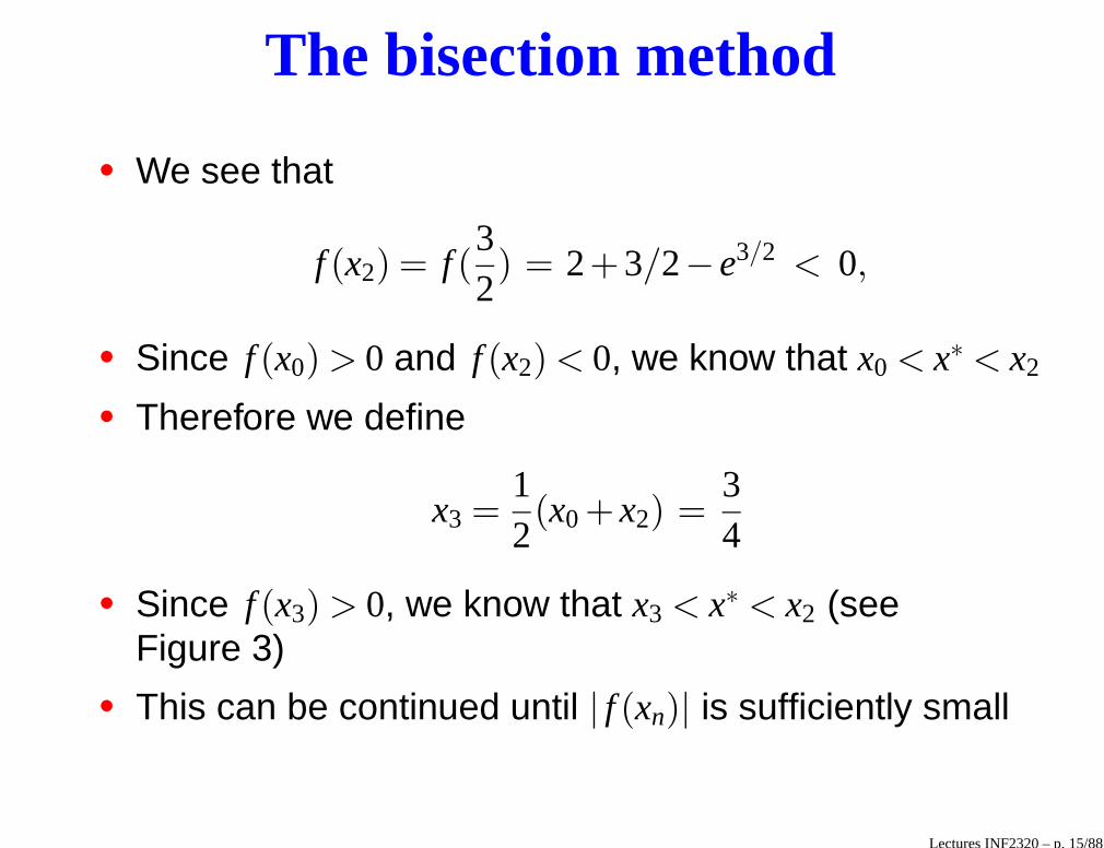
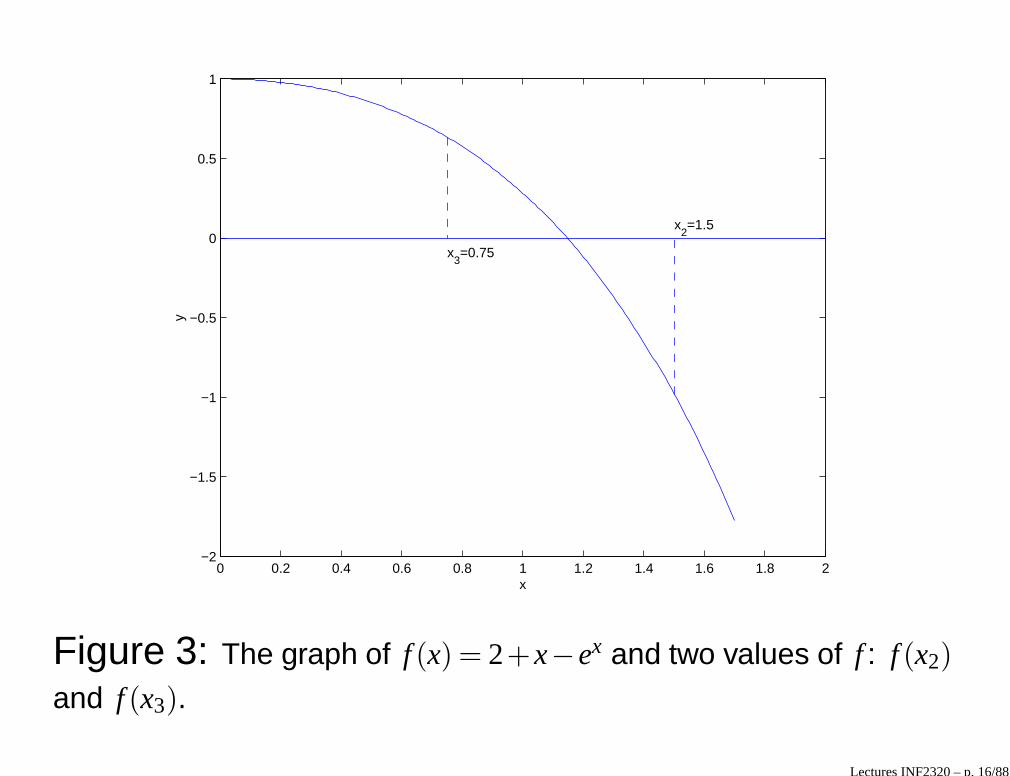
The bisection method
• We see that
f (x2) = f (32) = 2+3/2− e3/2 < 0,
• Since f (x0) > 0 and f (x2) < 0, we know that x0 < x∗ < x2
• Therefore we define
x3 =12(x0 + x2) =
34
• Since f (x3) > 0, we know that x3 < x∗ < x2 (seeFigure 3)
• This can be continued until | f (xn)| is sufficiently small
Lectures INF2320 – p. 15/88
0 0.2 0.4 0.6 0.8 1 1.2 1.4 1.6 1.8 2−2
−1.5
−1
−0.5
0
0.5
1
x3=0.75
x2=1.5
x
y
Figure 3: The graph of f (x) = 2+x−ex and two values of f : f (x2)
and f (x3).
Lectures INF2320 – p. 16/88
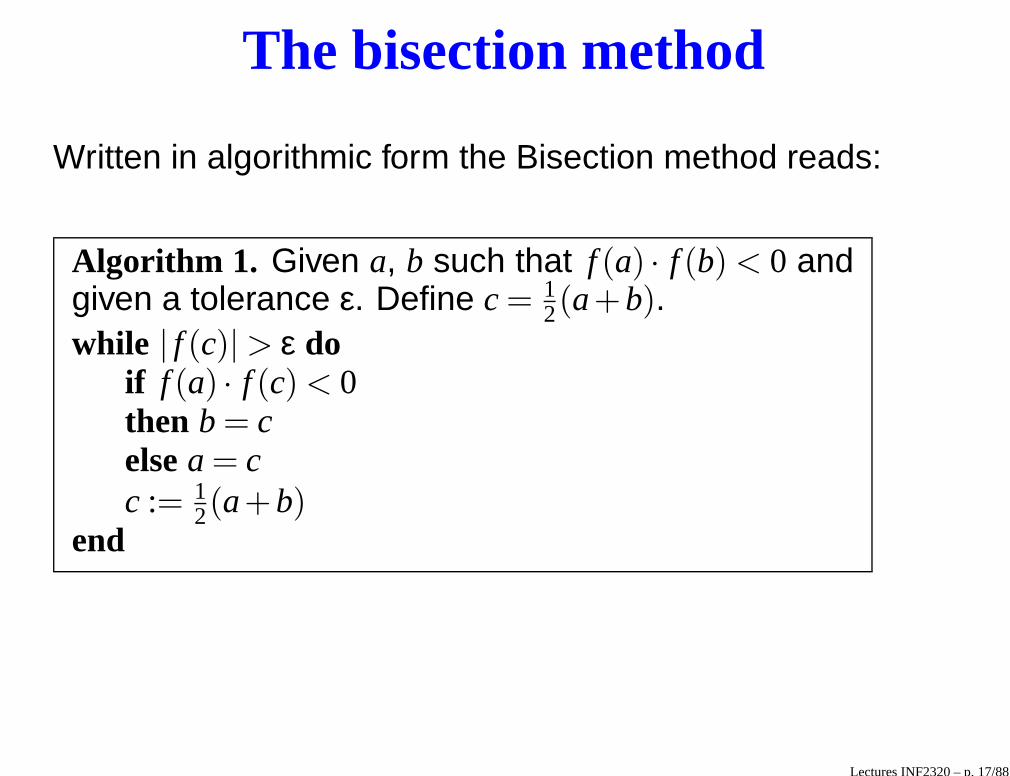
The bisection method
Written in algorithmic form the Bisection method reads:
Algorithm 1. Given a, b such that f (a) · f (b) < 0 andgiven a tolerance ε. Define c = 1
2(a+b).while | f (c)| > ε do
if f (a) · f (c) < 0then b = celsea = cc := 1
2(a+b)end
Lectures INF2320 – p. 17/88
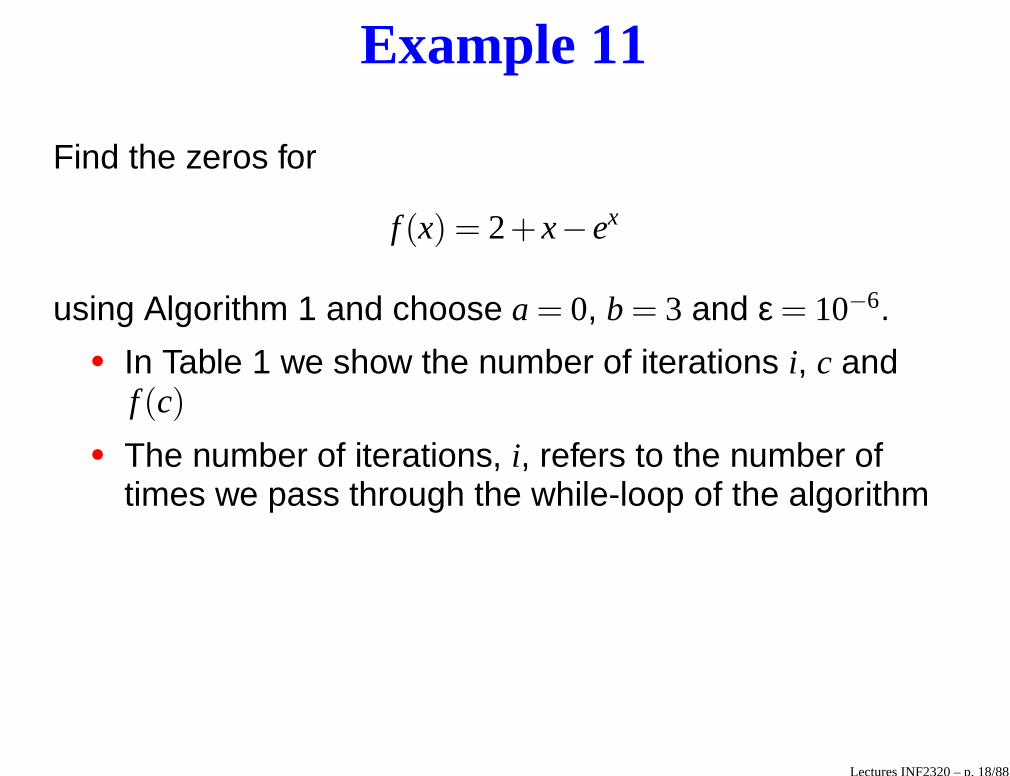
Example 11
Find the zeros for
f (x) = 2+ x− ex
using Algorithm 1 and choose a = 0, b = 3 and ε = 10−6.• In Table 1 we show the number of iterations i, c and
f (c)
• The number of iterations, i, refers to the number oftimes we pass through the while-loop of the algorithm
Lectures INF2320 – p. 18/88
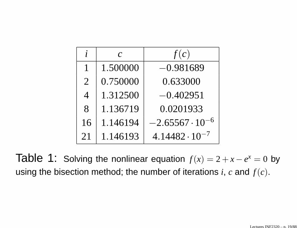
i c f (c)
1 1.500000 −0.9816892 0.750000 0.6330004 1.312500 −0.4029518 1.136719 0.020193316 1.146194 −2.65567·10−6
21 1.146193 4.14482·10−7
Table 1: Solving the nonlinear equation f (x) = 2+ x− ex = 0 by
using the bisection method; the number of iterations i, c and f (c).
Lectures INF2320 – p. 19/88
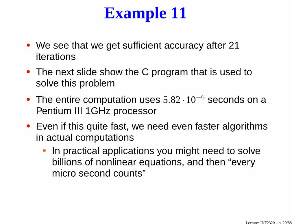
Example 11
• We see that we get sufficient accuracy after 21iterations
• The next slide show the C program that is used tosolve this problem
• The entire computation uses 5.82·10−6 seconds on aPentium III 1GHz processor
• Even if this quite fast, we need even faster algorithmsin actual computations• In practical applications you might need to solve
billions of nonlinear equations, and then “everymicro second counts”
Lectures INF2320 – p. 20/88
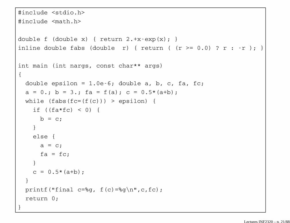
#include <stdio.h>
#include <math.h>
double f (double x) { return 2.+x-exp(x); }
inline double fabs (double r) { return ( (r >= 0.0) ? r : -r ); }
int main (int nargs, const char** args)
{
double epsilon = 1.0e-6; double a, b, c, fa, fc;
a = 0.; b = 3.; fa = f(a); c = 0.5*(a+b);
while (fabs(fc=(f(c))) > epsilon) {
if ((fa*fc) < 0) {
b = c;
}
else {
a = c;
fa = fc;
}
c = 0.5*(a+b);
}
printf("final c=%g, f(c)=%g\n",c,fc);
return 0;
}
Lectures INF2320 – p. 21/88
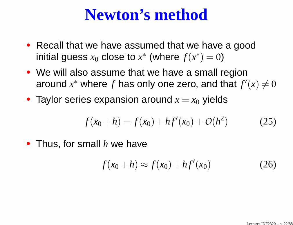
Newton’s method
• Recall that we have assumed that we have a goodinitial guess x0 close to x∗ (where f (x∗) = 0)
• We will also assume that we have a small regionaround x∗ where f has only one zero, and that f ′(x) 6= 0
• Taylor series expansion around x = x0 yields
f (x0 +h) = f (x0)+h f ′(x0)+O(h2) (25)
• Thus, for small h we have
f (x0 +h) ≈ f (x0)+h f ′(x0) (26)
Lectures INF2320 – p. 22/88
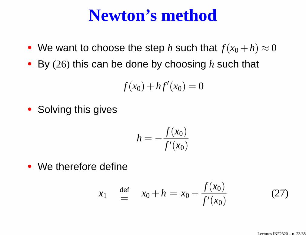
Newton’s method
• We want to choose the step h such that f (x0 +h) ≈ 0
• By (26) this can be done by choosing h such that
f (x0)+h f ′(x0) = 0
• Solving this gives
h = − f (x0)
f ′(x0)
• We therefore define
x1def= x0 +h = x0−
f (x0)
f ′(x0)(27)
Lectures INF2320 – p. 23/88
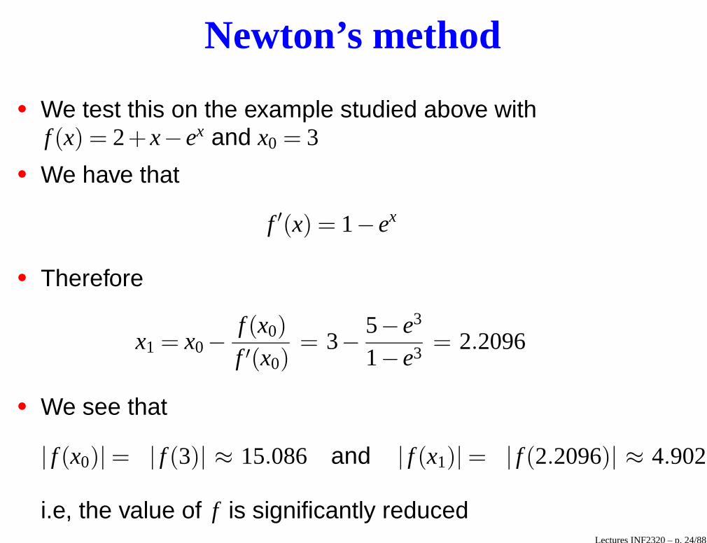
Newton’s method
• We test this on the example studied above withf (x) = 2+ x− ex and x0 = 3
• We have that
f ′(x) = 1− ex
• Therefore
x1 = x0−f (x0)
f ′(x0)= 3− 5− e3
1− e3= 2.2096
• We see that
| f (x0)| = | f (3)| ≈ 15.086 and | f (x1)| = | f (2.2096)| ≈ 4.902,
i.e, the value of f is significantly reducedLectures INF2320 – p. 24/88
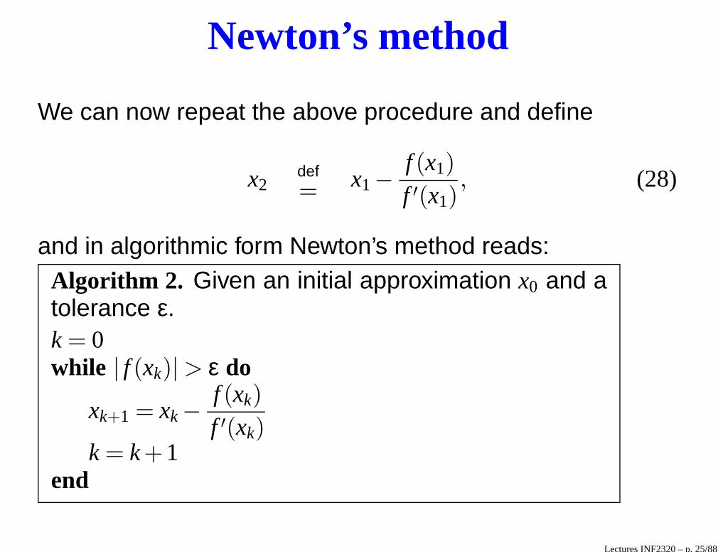
Newton’s method
We can now repeat the above procedure and define
x2def= x1−
f (x1)
f ′(x1), (28)
and in algorithmic form Newton’s method reads:Algorithm 2. Given an initial approximation x0 and atolerance ε.k = 0while | f (xk)| > ε do
xk+1 = xk −f (xk)
f ′(xk)k = k +1
end
Lectures INF2320 – p. 25/88
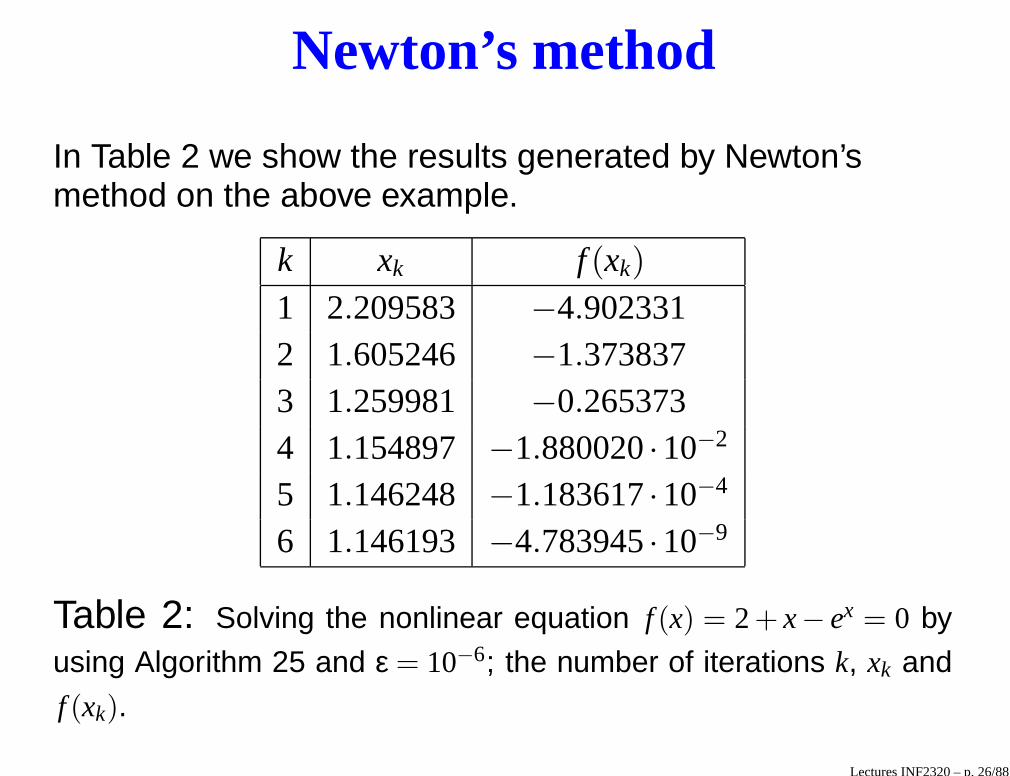
Newton’s method
In Table 2 we show the results generated by Newton’smethod on the above example.
k xk f (xk)
1 2.209583 −4.9023312 1.605246 −1.3738373 1.259981 −0.2653734 1.154897 −1.880020·10−2
5 1.146248 −1.183617·10−4
6 1.146193 −4.783945·10−9
Table 2: Solving the nonlinear equation f (x) = 2+ x− ex = 0 by
using Algorithm 25 and ε = 10−6; the number of iterations k, xk and
f (xk).
Lectures INF2320 – p. 26/88
Newton’s method
• We observe that the convergence is much faster forNewton’s method than for the Bisection method
• Generally, Newton’s method converges faster than theBisection method
• This will be studied in more detail in Project 1
Lectures INF2320 – p. 27/88
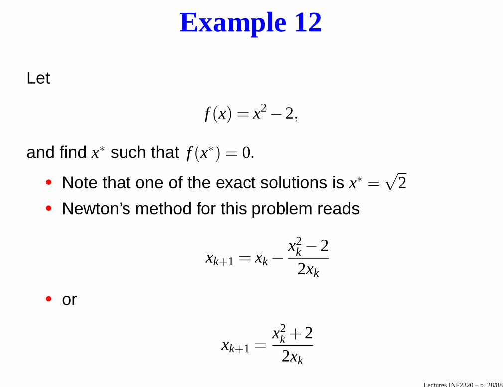
Example 12
Let
f (x) = x2−2,
and find x∗ such that f (x∗) = 0.
• Note that one of the exact solutions is x∗ =√
2
• Newton’s method for this problem reads
xk+1 = xk −x2
k −22xk
• or
xk+1 =x2
k +22xk
Lectures INF2320 – p. 28/88
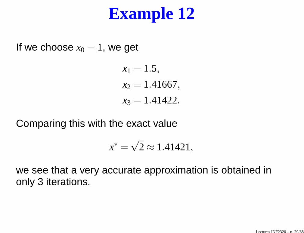
Example 12
If we choose x0 = 1, we get
x1 = 1.5,
x2 = 1.41667,
x3 = 1.41422.
Comparing this with the exact value
x∗ =√
2≈ 1.41421,
we see that a very accurate approximation is obtained inonly 3 iterations.
Lectures INF2320 – p. 29/88
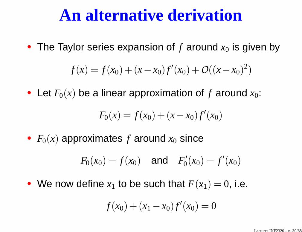
An alternative derivation
• The Taylor series expansion of f around x0 is given by
f (x) = f (x0)+(x− x0) f ′(x0)+O((x− x0)2)
• Let F0(x) be a linear approximation of f around x0:
F0(x) = f (x0)+(x− x0) f ′(x0)
• F0(x) approximates f around x0 since
F0(x0) = f (x0) and F ′0(x0) = f ′(x0)
• We now define x1 to be such that F(x1) = 0, i.e.
f (x0)+(x1− x0) f ′(x0) = 0
Lectures INF2320 – p. 30/88
An alternative derivation
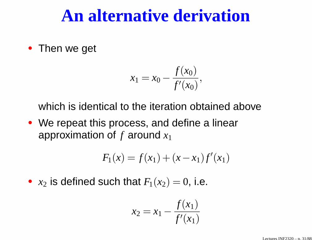
• Then we get
x1 = x0−f (x0)
f ′(x0),
which is identical to the iteration obtained above• We repeat this process, and define a linear
approximation of f around x1
F1(x) = f (x1)+(x− x1) f ′(x1)
• x2 is defined such that F1(x2) = 0, i.e.
x2 = x1−f (x1)
f ′(x1)
Lectures INF2320 – p. 31/88
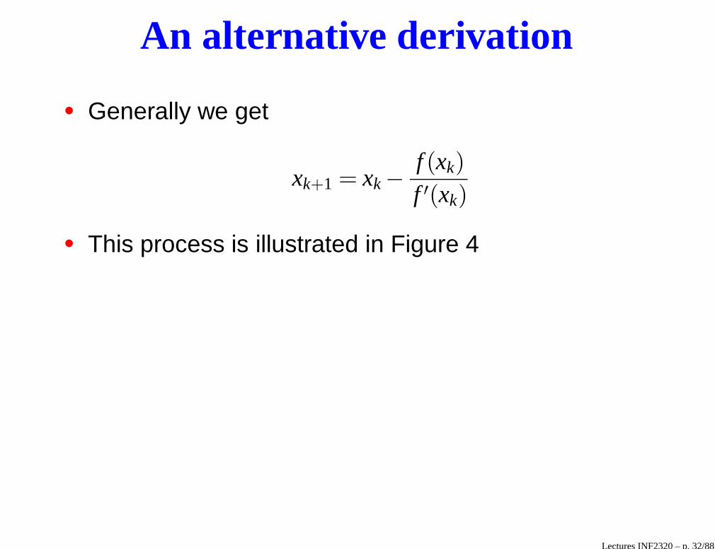
An alternative derivation
• Generally we get
xk+1 = xk −f (xk)
f ′(xk)
• This process is illustrated in Figure 4
Lectures INF2320 – p. 32/88
x0x1x2x3f (x)
Figure 4: Graphical illustration of Newton’s method.
Lectures INF2320 – p. 33/88
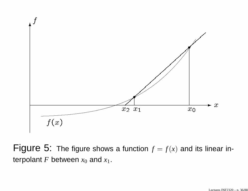
The Secant method
• The secant method is similar to Newton’s method, butthe linear approximation of f is defined differently
• Now we assume that we have two values x0 and x1
close to x∗, and define the linear function F0(x) suchthat
F0(x0) = f (x0) and F0(x1) = f (x1)
• The function F0(x) is therefore given by
F0(x) = f (x1)+f (x1)− f (x0)
x1− x0(x− x1)
• F0(x) is called the linear interpolant of f
Lectures INF2320 – p. 34/88
The Secant method
• Since F0(x) ≈ f (x), we can compute a newapproximation x2 to x∗ by solving the linear equation
F(x2) = 0
• This means that we must solve
f (x1)+f (x1)− f (x0)
x1− x0(x2− x1) = 0,
with respect to x2 (see Figure 5)• This gives
x2 = x1−f (x1)(x1− x0)
f (x1)− f (x0)
Lectures INF2320 – p. 35/88
�
�
x
f
�
��
��
��
��
��
��
��
��
�
x � x � x �
f
�
x
�
Figure 5: The figure shows a function f = f (x) and its linear in-
terpolant F between x0 and x1.
Lectures INF2320 – p. 36/88
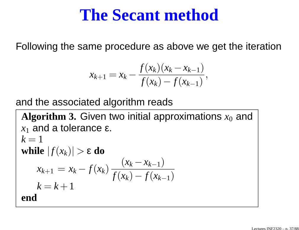
The Secant method
Following the same procedure as above we get the iteration
xk+1 = xk −f (xk)(xk − xk−1)
f (xk)− f (xk−1),
and the associated algorithm readsAlgorithm 3. Given two initial approximations x0 andx1 and a tolerance ε.k = 1while | f (xk)| > ε do
xk+1 = xk − f (xk)(xk − xk−1)
f (xk)− f (xk−1)k = k +1
end
Lectures INF2320 – p. 37/88
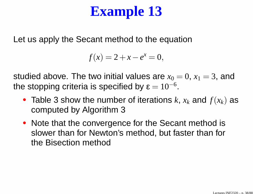
Example 13
Let us apply the Secant method to the equation
f (x) = 2+ x− ex = 0,
studied above. The two initial values are x0 = 0, x1 = 3, andthe stopping criteria is specified by ε = 10−6.
• Table 3 show the number of iterations k, xk and f (xk) ascomputed by Algorithm 3
• Note that the convergence for the Secant method isslower than for Newton’s method, but faster than forthe Bisection method
Lectures INF2320 – p. 38/88
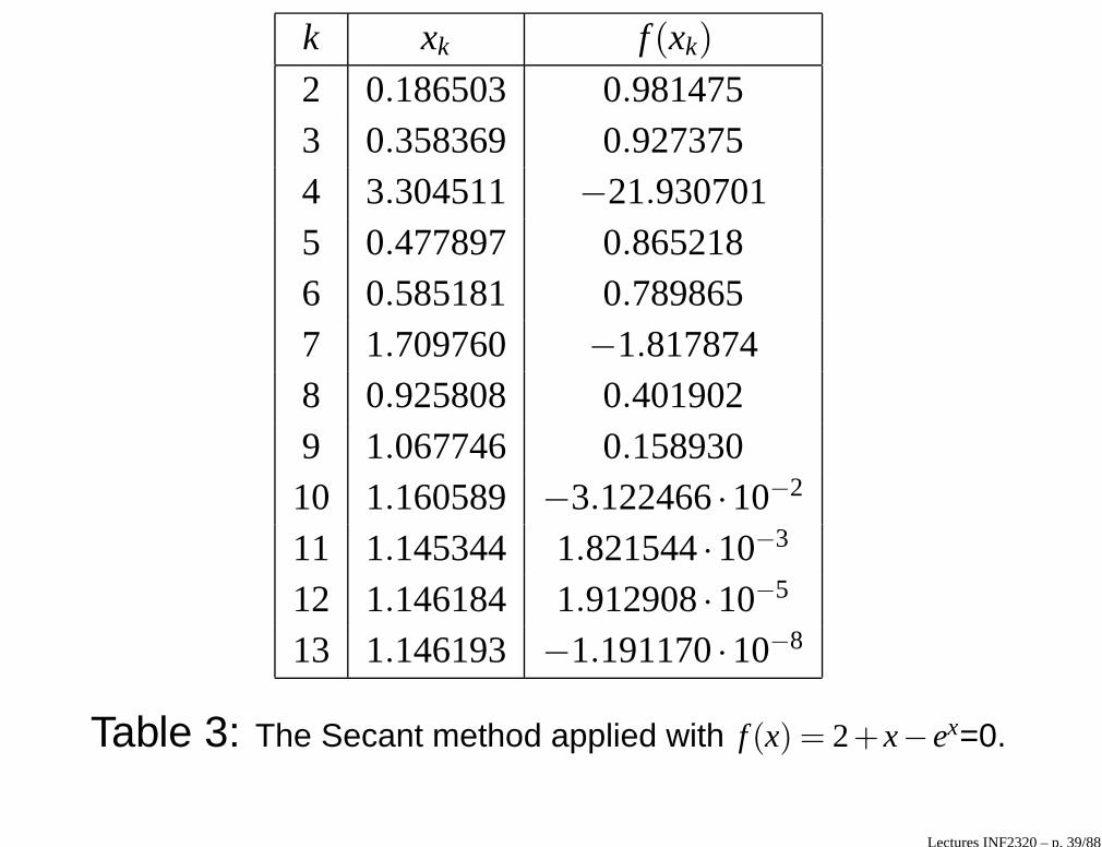
k xk f (xk)
2 0.186503 0.9814753 0.358369 0.9273754 3.304511 −21.9307015 0.477897 0.8652186 0.585181 0.7898657 1.709760 −1.8178748 0.925808 0.4019029 1.067746 0.15893010 1.160589 −3.122466·10−2
11 1.145344 1.821544·10−3
12 1.146184 1.912908·10−5
13 1.146193 −1.191170·10−8
Table 3: The Secant method applied with f (x) = 2+ x− ex=0.
Lectures INF2320 – p. 39/88
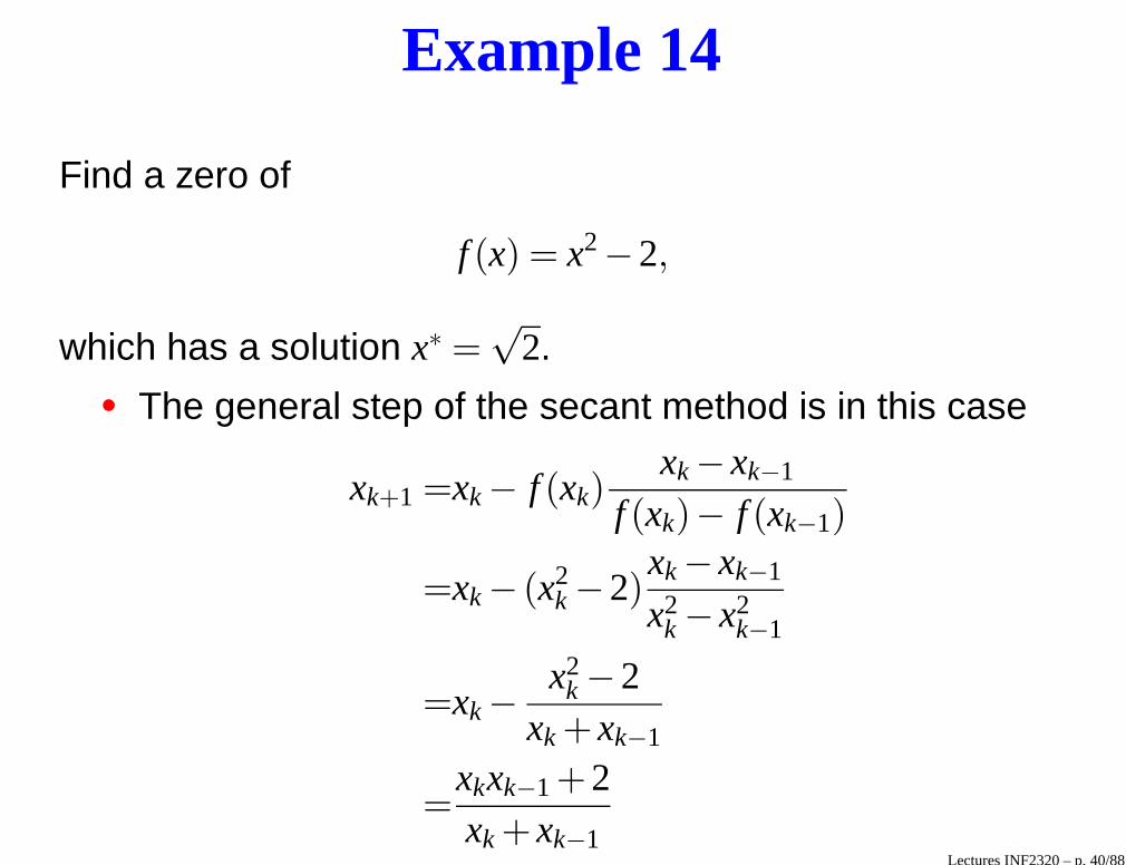
Example 14
Find a zero of
f (x) = x2−2,
which has a solution x∗ =√
2.• The general step of the secant method is in this case
xk+1 =xk − f (xk)xk − xk−1
f (xk)− f (xk−1)
=xk − (x2k −2)
xk − xk−1
x2k − x2
k−1
=xk −x2
k −2xk + xk−1
=xkxk−1 +2xk + xk−1
Lectures INF2320 – p. 40/88
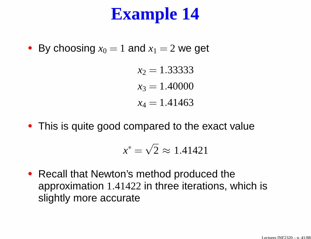
Example 14
• By choosing x0 = 1 and x1 = 2 we get
x2 = 1.33333
x3 = 1.40000
x4 = 1.41463
• This is quite good compared to the exact value
x∗ =√
2 ≈ 1.41421
• Recall that Newton’s method produced theapproximation 1.41422in three iterations, which isslightly more accurate
Lectures INF2320 – p. 41/88
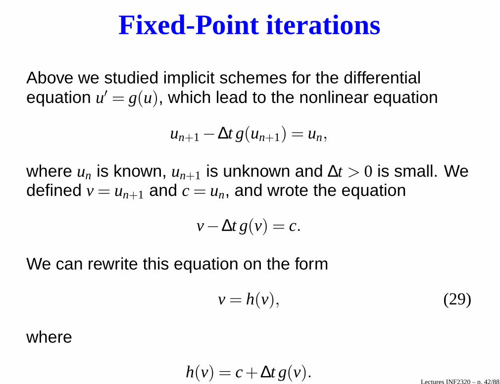
Fixed-Point iterations
Above we studied implicit schemes for the differentialequation u′ = g(u), which lead to the nonlinear equation
un+1−∆t g(un+1) = un,
where un is known, un+1 is unknown and ∆t > 0 is small. Wedefined v = un+1 and c = un, and wrote the equation
v−∆t g(v) = c.
We can rewrite this equation on the form
v = h(v), (29)
where
h(v) = c+∆t g(v).Lectures INF2320 – p. 42/88
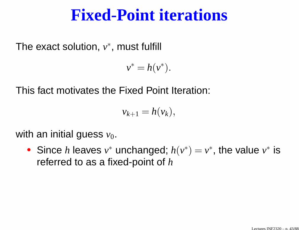
Fixed-Point iterations
The exact solution, v∗, must fulfill
v∗ = h(v∗).
This fact motivates the Fixed Point Iteration:
vk+1 = h(vk),
with an initial guess v0.• Since h leaves v∗ unchanged; h(v∗) = v∗, the value v∗ is
referred to as a fixed-point of h
Lectures INF2320 – p. 43/88
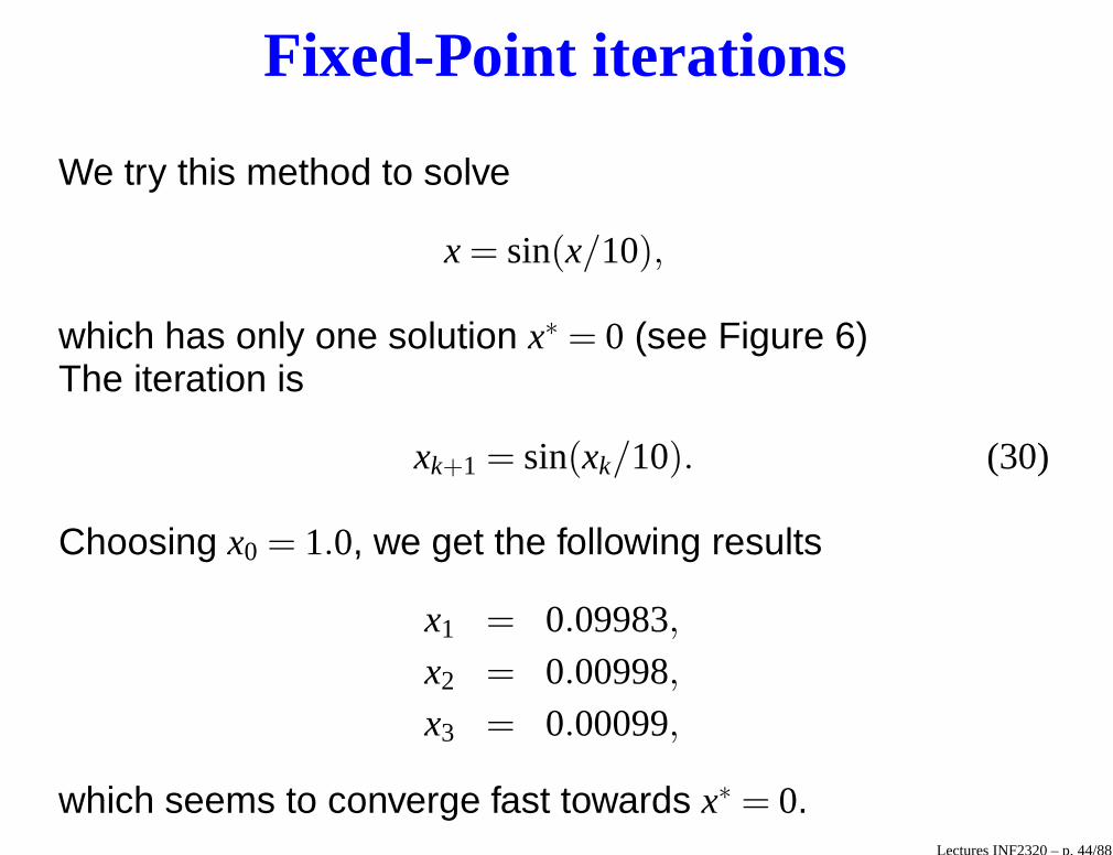
Fixed-Point iterations
We try this method to solve
x = sin(x/10),
which has only one solution x∗ = 0 (see Figure 6)The iteration is
xk+1 = sin(xk/10). (30)
Choosing x0 = 1.0, we get the following results
x1 = 0.09983,x2 = 0.00998,x3 = 0.00099,
which seems to converge fast towards x∗ = 0.Lectures INF2320 – p. 44/88
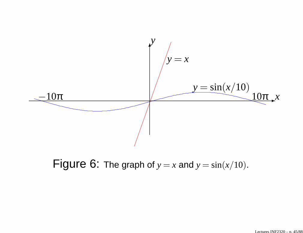
6
-x
y
y = x
y = sin(x/10)−10π 10π
Figure 6: The graph of y = x and y = sin(x/10).
Lectures INF2320 – p. 45/88
Fixed-Point iterations
We now try to understand the behavior of the iteration.From calculus we recall for small x we have
sin(x/10) ≈ x/10.
Using this fact in (30), we get
xk+1 ≈ xk/10,
and therefore
xk ≈ (1/10)k.
We see that this iteration converges towards zero.
Lectures INF2320 – p. 46/88
Convergence of Fixed-Point iterations
We have seen that h(v) = v can be solved with theFixed-Point iteration
vk+1 = h(vk)
We now analyze under what conditions the values {vk}generated by the Fixed-Point iterations converge towards asolution v∗ of the equation.Definition: h = h(v) is called a contractive mapping on aclosed interval I if
(i) |h(v)−h(w)| ≤ δ |v−w| for any v,w ∈ I, where 0 < δ < 1,
and
(ii) v ∈ I ⇒ h(v) ∈ I.
Lectures INF2320 – p. 47/88
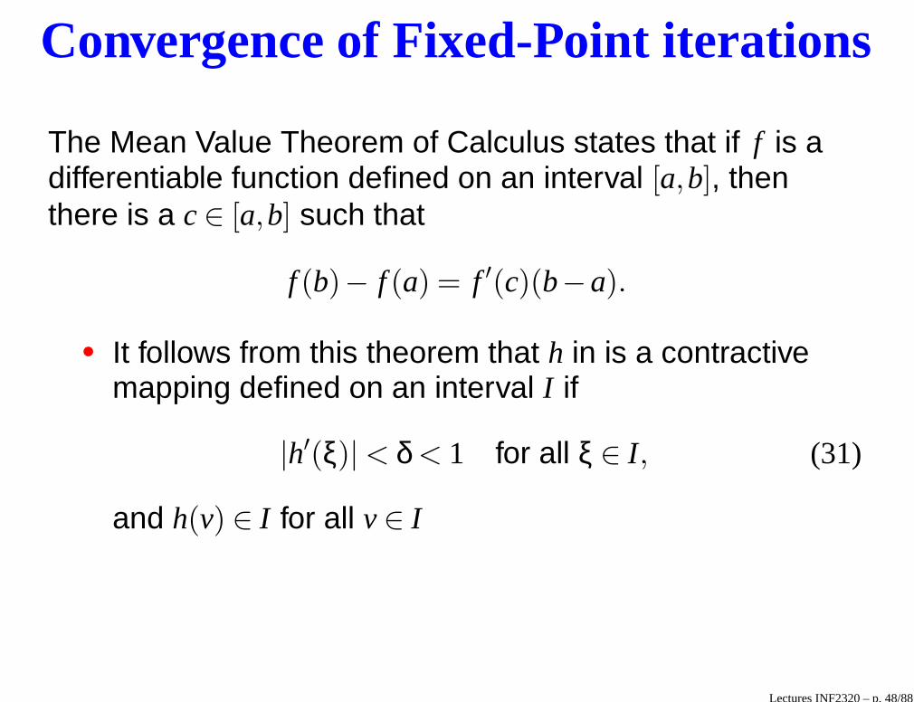
Convergence of Fixed-Point iterations
The Mean Value Theorem of Calculus states that if f is adifferentiable function defined on an interval [a,b], thenthere is a c ∈ [a,b] such that
f (b)− f (a) = f ′(c)(b−a).
• It follows from this theorem that h in is a contractivemapping defined on an interval I if
|h′(ξ)| < δ < 1 for all ξ ∈ I, (31)
and h(v) ∈ I for all v ∈ I
Lectures INF2320 – p. 48/88
Convergence of Fixed-Point iterations
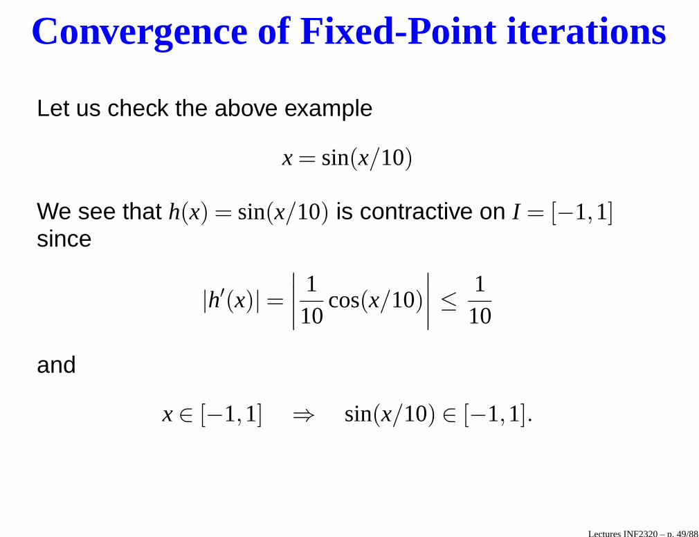
Let us check the above example
x = sin(x/10)
We see that h(x) = sin(x/10) is contractive on I = [−1,1]since
|h′(x)| =∣
∣
∣
∣
110
cos(x/10)
∣
∣
∣
∣
≤ 110
and
x ∈ [−1,1] ⇒ sin(x/10) ∈ [−1,1].
Lectures INF2320 – p. 49/88
Convergence of Fixed-Point iterations
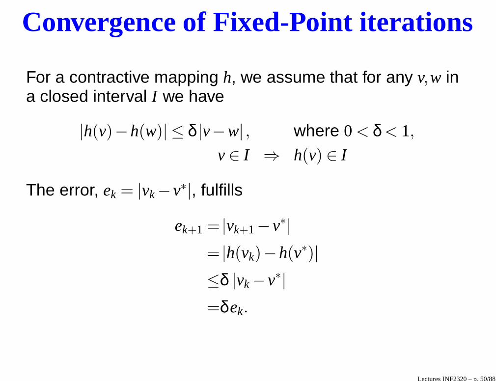
For a contractive mapping h, we assume that for any v,w ina closed interval I we have
|h(v)−h(w)| ≤ δ |v−w| , where 0 < δ < 1,
v ∈ I ⇒ h(v) ∈ I
The error, ek = |vk − v∗|, fulfills
ek+1 = |vk+1− v∗|= |h(vk)−h(v∗)|≤δ |vk − v∗|=δek.
Lectures INF2320 – p. 50/88
Convergence of Fixed-Point iterations
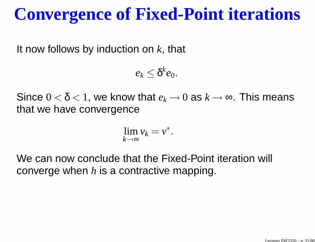
It now follows by induction on k, that
ek ≤ δke0.
Since 0 < δ < 1, we know that ek → 0 as k → ∞. This meansthat we have convergence
limk→∞
vk = v∗.
We can now conclude that the Fixed-Point iteration willconverge when h is a contractive mapping.
Lectures INF2320 – p. 51/88
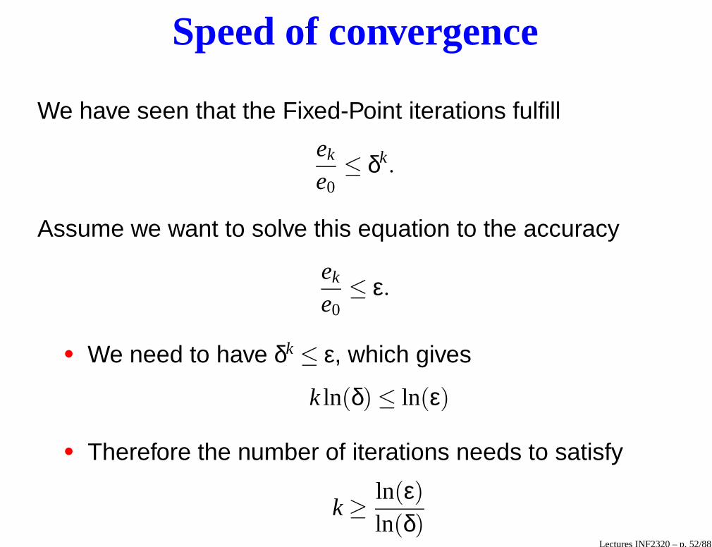
Speed of convergence
We have seen that the Fixed-Point iterations fulfill
ek
e0≤ δk.
Assume we want to solve this equation to the accuracy
ek
e0≤ ε.
• We need to have δk ≤ ε, which gives
k ln(δ) ≤ ln(ε)
• Therefore the number of iterations needs to satisfy
k ≥ ln(ε)ln(δ)
Lectures INF2320 – p. 52/88
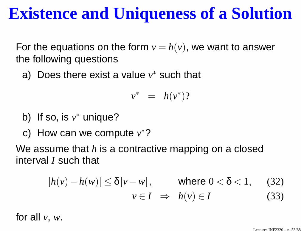
Existence and Uniqueness of a Solution
For the equations on the form v = h(v), we want to answerthe following questions
a) Does there exist a value v∗ such that
v∗ = h(v∗)?
b) If so, is v∗ unique?
c) How can we compute v∗?
We assume that h is a contractive mapping on a closedinterval I such that
|h(v)−h(w)| ≤ δ |v−w| , where 0 < δ < 1, (32)
v ∈ I ⇒ h(v) ∈ I (33)
for all v, w.Lectures INF2320 – p. 53/88
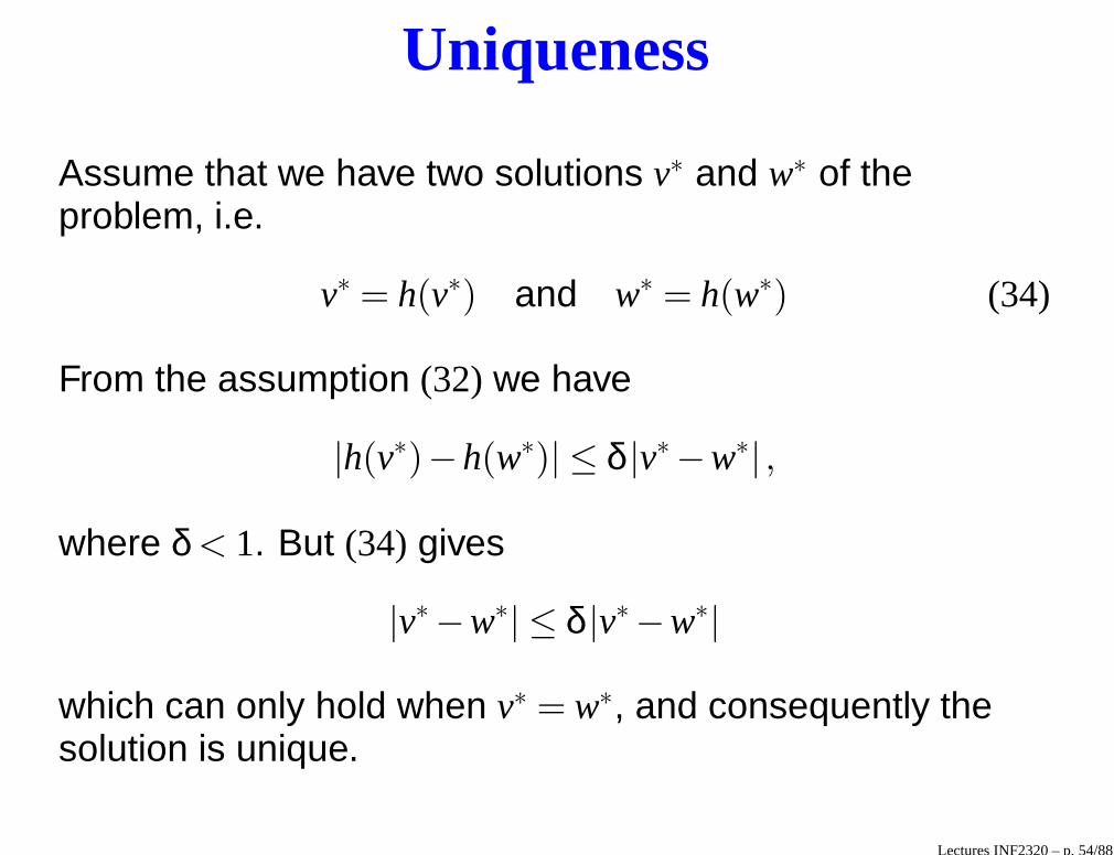
Uniqueness
Assume that we have two solutions v∗ and w∗ of theproblem, i.e.
v∗ = h(v∗) and w∗ = h(w∗) (34)
From the assumption (32) we have
|h(v∗)−h(w∗)| ≤ δ |v∗−w∗| ,
where δ < 1. But (34) gives
|v∗−w∗| ≤ δ |v∗−w∗|
which can only hold when v∗ = w∗, and consequently thesolution is unique.
Lectures INF2320 – p. 54/88
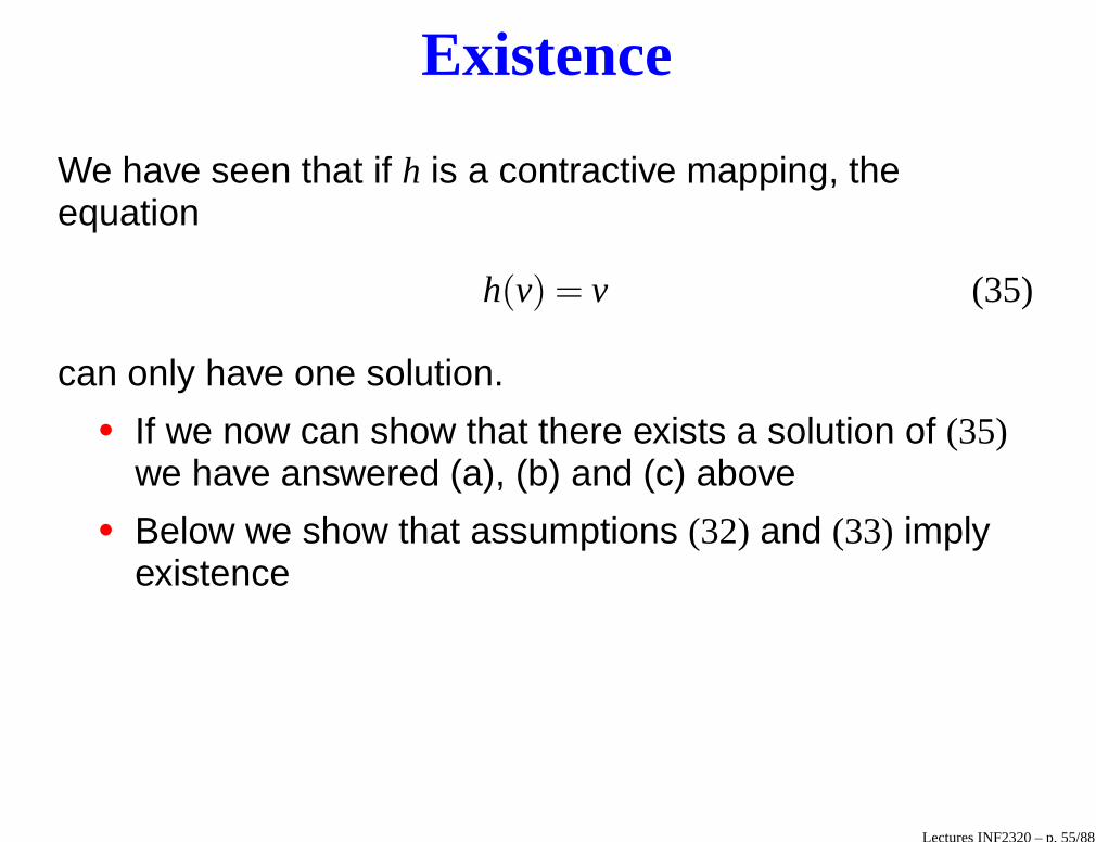
Existence
We have seen that if h is a contractive mapping, theequation
h(v) = v (35)
can only have one solution.• If we now can show that there exists a solution of (35)
we have answered (a), (b) and (c) above• Below we show that assumptions (32) and (33) imply
existence
Lectures INF2320 – p. 55/88
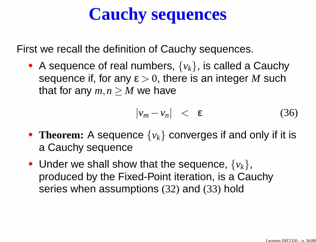
Cauchy sequences
First we recall the definition of Cauchy sequences.• A sequence of real numbers, {vk}, is called a Cauchy
sequence if, for any ε > 0, there is an integer M suchthat for any m,n ≥ M we have
|vm − vn| < ε (36)
• Theorem: A sequence {vk} converges if and only if it isa Cauchy sequence
• Under we shall show that the sequence, {vk},produced by the Fixed-Point iteration, is a Cauchyseries when assumptions (32) and (33) hold
Lectures INF2320 – p. 56/88
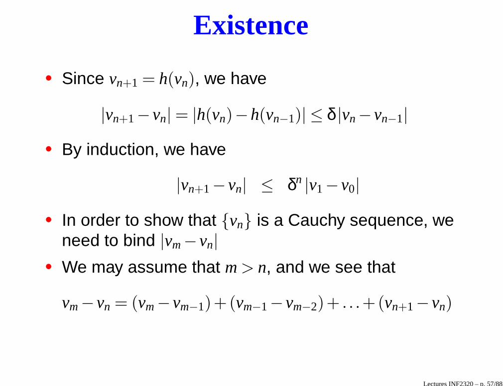
Existence
• Since vn+1 = h(vn), we have
|vn+1− vn| = |h(vn)−h(vn−1)| ≤ δ |vn − vn−1|
• By induction, we have
|vn+1− vn| ≤ δn |v1− v0|
• In order to show that {vn} is a Cauchy sequence, weneed to bind |vm − vn|
• We may assume that m > n, and we see that
vm − vn = (vm − vm−1)+(vm−1− vm−2)+ . . .+(vn+1− vn)
Lectures INF2320 – p. 57/88
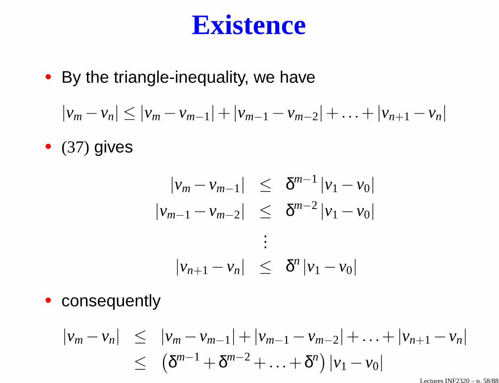
Existence
• By the triangle-inequality, we have
|vm − vn| ≤ |vm − vm−1|+ |vm−1− vm−2|+ . . .+ |vn+1− vn|
• (37) gives
|vm − vm−1| ≤ δm−1 |v1− v0||vm−1− vm−2| ≤ δm−2 |v1− v0|
...|vn+1− vn| ≤ δn |v1− v0|
• consequently
|vm − vn| ≤ |vm − vm−1|+ |vm−1− vm−2|+ . . .+ |vn+1− vn|≤(
δm−1 +δm−2 + . . .+δn)
|v1− v0|Lectures INF2320 – p. 58/88
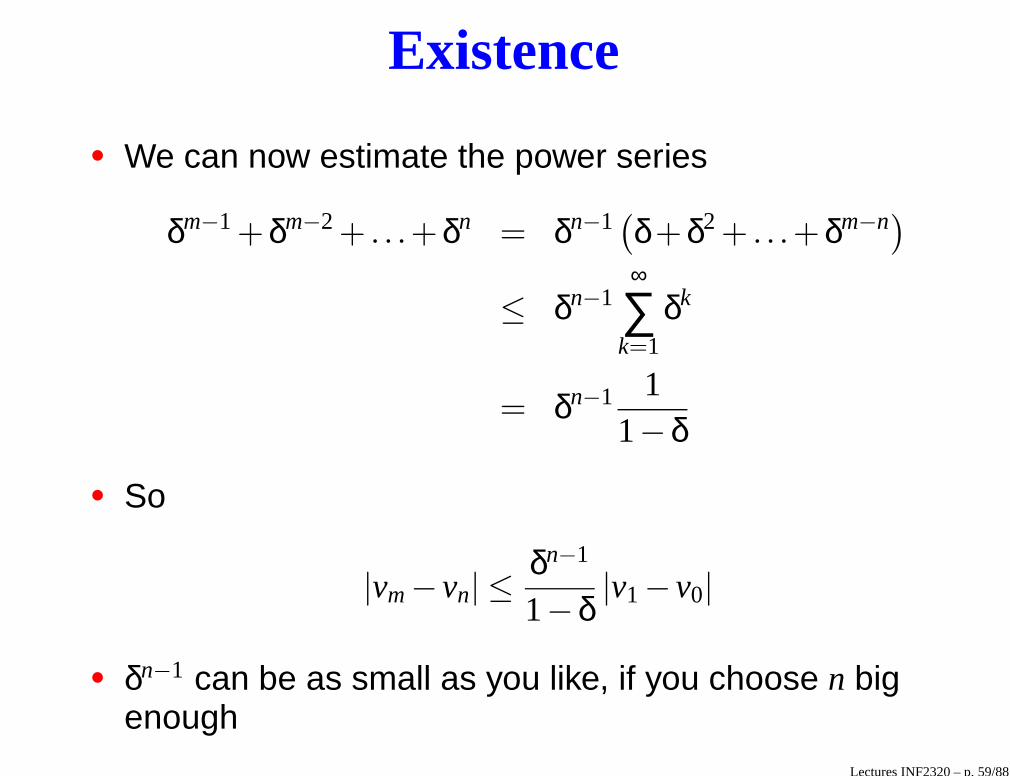
Existence
• We can now estimate the power series
δm−1 +δm−2 + . . .+δn = δn−1(
δ+δ2 + . . .+δm−n)
≤ δn−1∞
∑k=1
δk
= δn−1 11−δ
• So
|vm − vn| ≤δn−1
1−δ|v1− v0|
• δn−1 can be as small as you like, if you choose n bigenough
Lectures INF2320 – p. 59/88
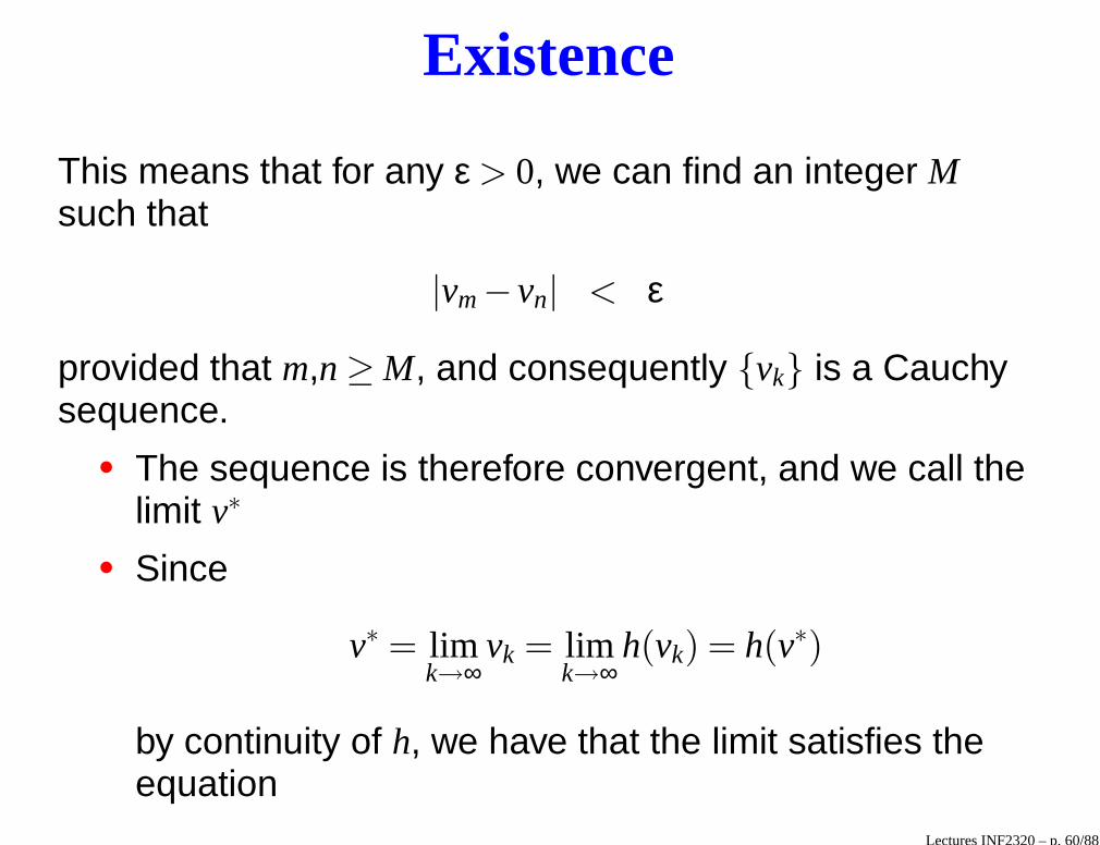
Existence
This means that for any ε > 0, we can find an integer Msuch that
|vm − vn| < ε
provided that m,n ≥ M, and consequently {vk} is a Cauchysequence.
• The sequence is therefore convergent, and we call thelimit v∗
• Since
v∗ = limk→∞
vk = limk→∞
h(vk) = h(v∗)
by continuity of h, we have that the limit satisfies theequation
Lectures INF2320 – p. 60/88
Systems of nonlinear equations
We start our study of nonlinear equations, by considering alinear system that arises from the discretization of a linear2×2 system of ordinary differential equations,
u′(t) = −v(t), u(0) = u0,
v′(t) = u(t), v(0) = v0.(37)
An implicit Euler scheme for this system reads
un+1−un
∆t= −vn+1,
vn+1− vn
∆t= un+1, (38)
and can be rewritten on the form
un+1 +∆t vn+1 = un,
−∆t un+1 + vn+1 = vn.(39)
Lectures INF2320 – p. 61/88
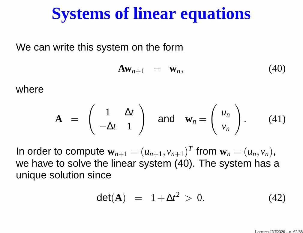
Systems of linear equations
We can write this system on the form
Awn+1 = wn, (40)
where
A =
(
1 ∆t−∆t 1
)
and wn =
(
un
vn
)
. (41)
In order to compute wn+1 = (un+1,vn+1)T from wn = (un,vn),
we have to solve the linear system (40). The system has aunique solution since
det(A) = 1+∆t2 > 0. (42)
Lectures INF2320 – p. 62/88
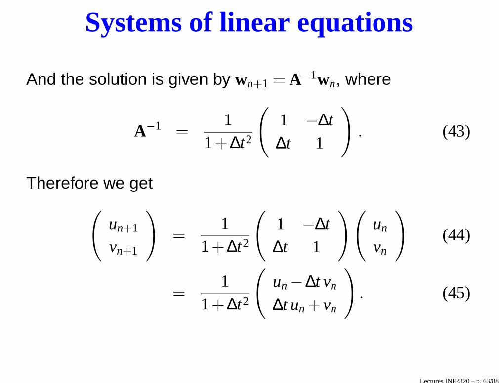
Systems of linear equations
And the solution is given by wn+1 = A−1wn, where
A−1 =1
1+∆t2
(
1 −∆t∆t 1
)
. (43)
Therefore we get(
un+1
vn+1
)
=1
1+∆t2
(
1 −∆t∆t 1
)(
un
vn
)
(44)
=1
1+∆t2
(
un −∆t vn
∆t un + vn
)
. (45)
Lectures INF2320 – p. 63/88
Systems of linear equations
We write this as
un+1 = 11+∆t2(un −∆t vn),
vn+1 = 11+∆t2(vn +∆t un).
(46)
By choosing u0 = 1 and v0 = 0, we have the analyticalsolutions
u(t) = cos(t), v(t) = sin(t). (47)
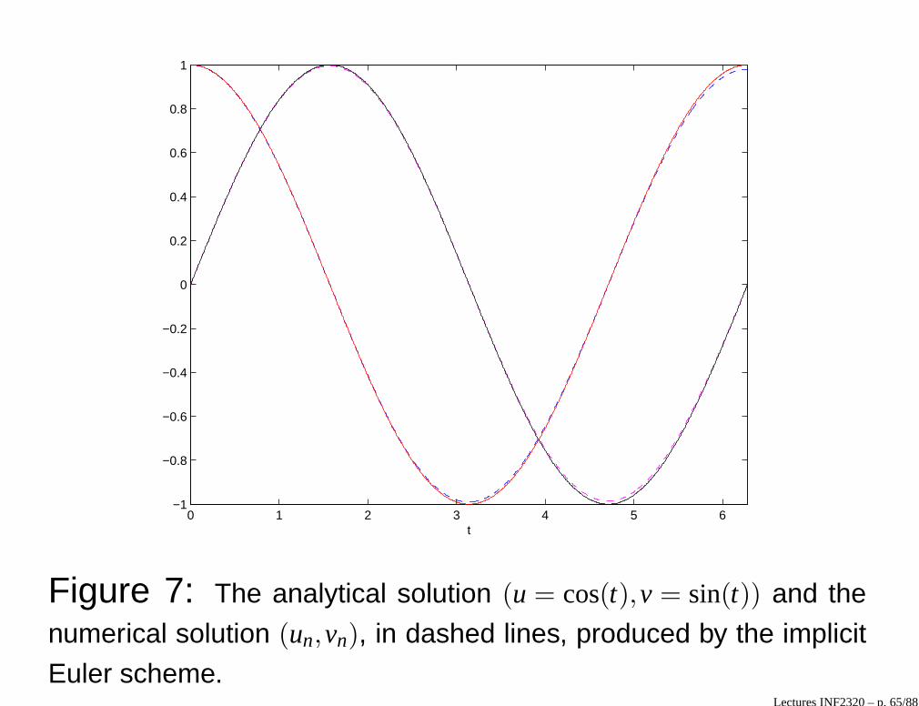
In Figure 7 we have plotted (u,v) and (un,vn) for 0≤ t ≤ 2π,∆t = π/500. We see that the scheme provides goodapproximations.
Lectures INF2320 – p. 64/88
0 1 2 3 4 5 6−1
−0.8
−0.6
−0.4
−0.2
0
0.2
0.4
0.6
0.8
1
t
Figure 7: The analytical solution (u = cos(t),v = sin(t)) and the
numerical solution (un,vn), in dashed lines, produced by the implicit
Euler scheme.Lectures INF2320 – p. 65/88
A nonlinear system
Now we study a nonlinear system of ordinary differentialequations
u′ = −v3, u(0) = u0,
v′ = u3, v(0) = v0.(48)
An implicit Euler scheme for this system reads
un+1−un
∆t= −v3
n+1,vn+1− vn
∆t= u3
n+1, (49)
which can be rewritten on the form
un+1 +∆t v3n+1−un = 0,
vn+1−∆t u3n+1− vn = 0.
(50)
Lectures INF2320 – p. 66/88
A nonlinear system
• Observe that in order to compute (un+1,vn+1) based on(un,vn), we need to solve a nonlinear system ofequations
We would like to write the system on the generic form
f (x,y) = 0,
g(x,y) = 0.(51)
This is done by setting
f (x,y) = x+∆t y3−α,
g(x,y) = y−∆t x3−β,(52)
α = un and β = vn.
Lectures INF2320 – p. 67/88

Newton’s method
When deriving Newton’s method for solving a scalarequation
p(x) = 0 (53)
we exploited Taylor series expansion
p(x0 +h) = p(x0)+hp′(x0)+O(h2), (54)
to make a linear approximation of the function p, and solvethe linear approximation of (53). This lead to the iteration
xk+1 = xk −p(xk)
p′(xk). (55)
Lectures INF2320 – p. 68/88
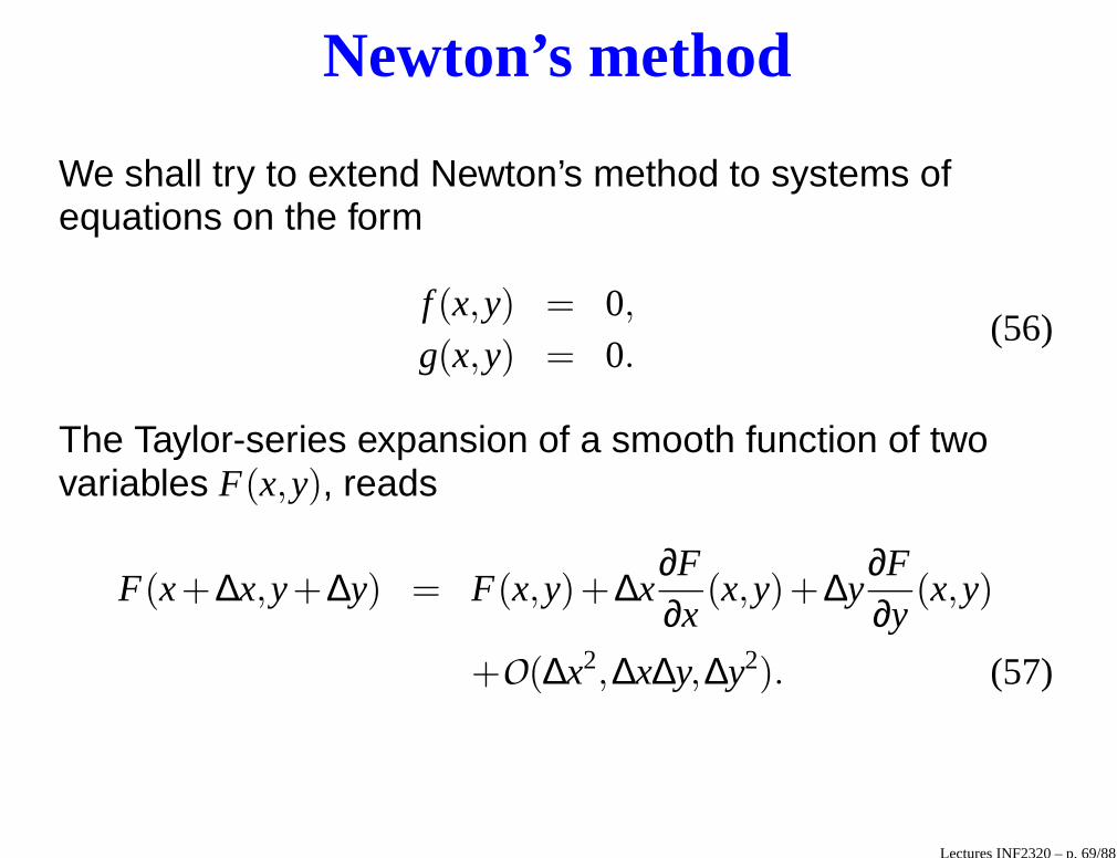
Newton’s method
We shall try to extend Newton’s method to systems ofequations on the form
f (x,y) = 0,
g(x,y) = 0.(56)
The Taylor-series expansion of a smooth function of twovariables F(x,y), reads
F(x+∆x,y+∆y) = F(x,y)+∆x∂F∂x
(x,y)+∆y∂F∂y
(x,y)
+O(∆x2,∆x∆y,∆y2). (57)
Lectures INF2320 – p. 69/88
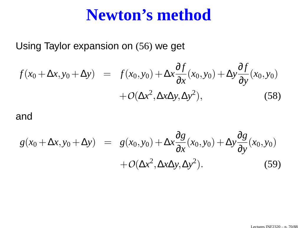
Newton’s method
Using Taylor expansion on (56) we get
f (x0 +∆x,y0+∆y) = f (x0,y0)+∆x∂ f∂x
(x0,y0)+∆y∂ f∂y
(x0,y0)
+O(∆x2,∆x∆y,∆y2), (58)
and
g(x0 +∆x,y0+∆y) = g(x0,y0)+∆x∂g∂x
(x0,y0)+∆y∂g∂y
(x0,y0)
+O(∆x2,∆x∆y,∆y2). (59)
Lectures INF2320 – p. 70/88
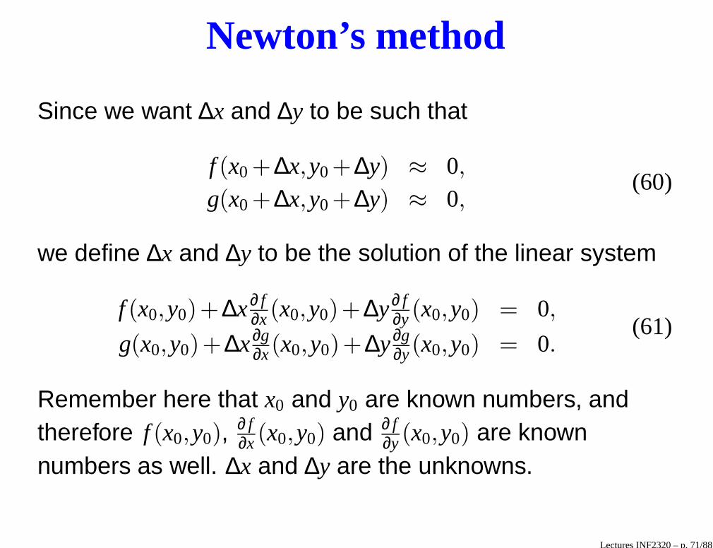
Newton’s method
Since we want ∆x and ∆y to be such that
f (x0 +∆x,y0+∆y) ≈ 0,
g(x0 +∆x,y0+∆y) ≈ 0,(60)
we define ∆x and ∆y to be the solution of the linear system
f (x0,y0)+∆x∂ f∂x (x0,y0)+∆y∂ f
∂y (x0,y0) = 0,
g(x0,y0)+∆x∂g∂x(x0,y0)+∆y∂g
∂y(x0,y0) = 0.(61)
Remember here that x0 and y0 are known numbers, andtherefore f (x0,y0),
∂ f∂x (x0,y0) and ∂ f
∂y (x0,y0) are knownnumbers as well. ∆x and ∆y are the unknowns.
Lectures INF2320 – p. 71/88
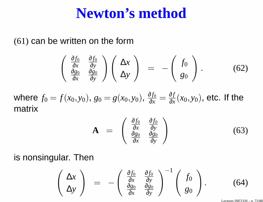
Newton’s method
(61) can be written on the form(
∂ f0∂x
∂ f0∂y
∂g0∂x
∂g0∂y
)(
∆x∆y
)
= −(
f0g0
)
. (62)
where f0 = f (x0,y0), g0 = g(x0,y0),∂ f0∂x = ∂ f
∂x (x0,y0), etc. If thematrix
A =
(
∂ f0∂x
∂ f0∂y
∂g0∂x
∂g0∂y
)
(63)
is nonsingular. Then(
∆x∆y
)
= −(
∂ f0∂x
∂ f0∂y
∂g0∂x
∂g0∂y
)−1(
f0g0
)
. (64)
Lectures INF2320 – p. 72/88
Newton’s method
We can now define(
x1
y1
)
=
(
x0
y0
)
+
(
∆x∆y
)
=
(
x0
y0
)
−(
∂ f0∂x
∂ f0∂y
∂g0∂x
∂g0∂y
)−1(
f0g0
)
.
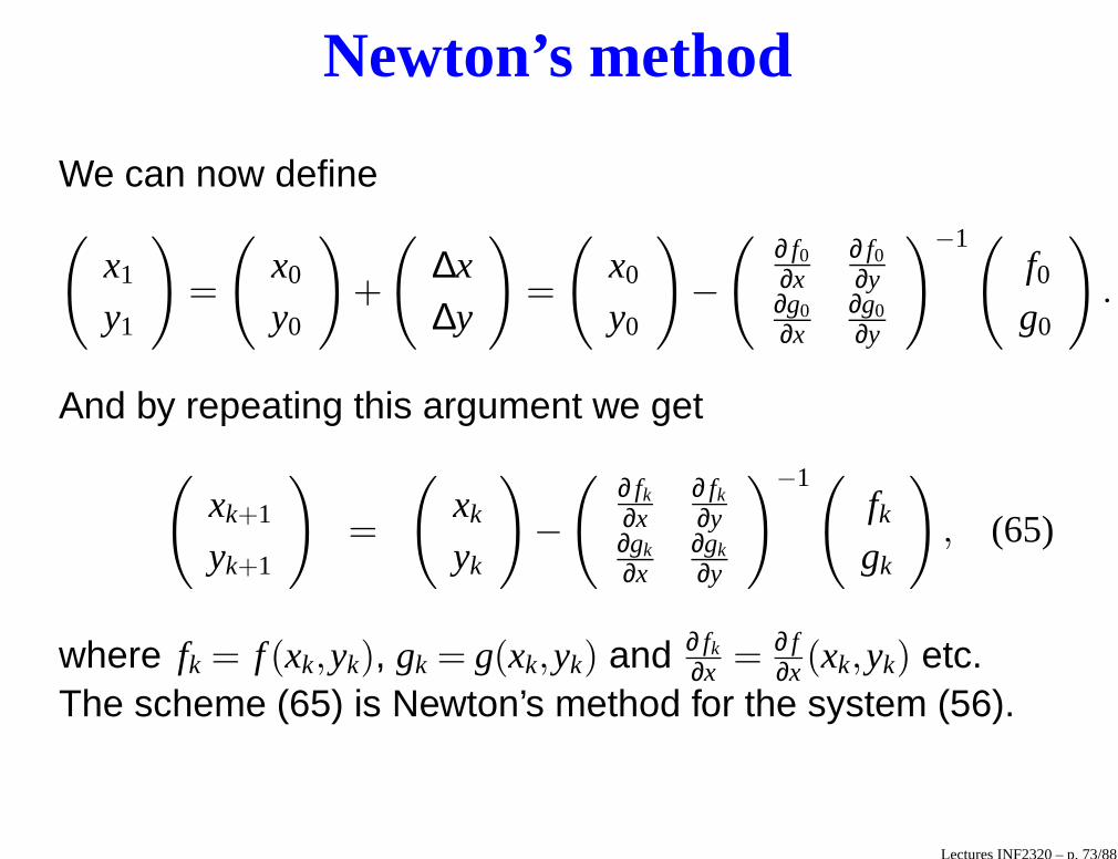
And by repeating this argument we get
(
xk+1
yk+1
)
=
(
xk
yk
)
−(
∂ fk
∂x∂ fk
∂y∂gk
∂x∂gk
∂y
)−1(
fk
gk
)
, (65)
where fk = f (xk,yk), gk = g(xk,yk) and ∂ fk
∂x = ∂ f∂x (xk,yk) etc.
The scheme (65) is Newton’s method for the system (56).
Lectures INF2320 – p. 73/88
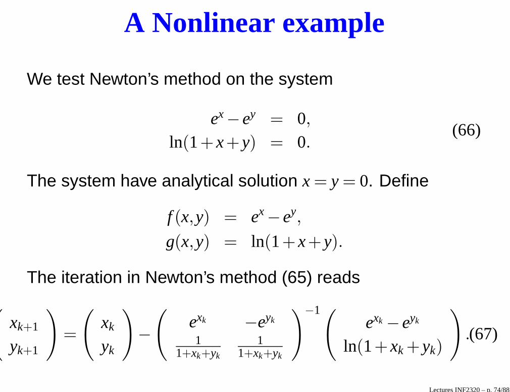
A Nonlinear example
We test Newton’s method on the system
ex − ey = 0,
ln(1+ x+ y) = 0.(66)
The system have analytical solution x = y = 0. Define
f (x,y) = ex − ey,
g(x,y) = ln(1+ x+ y).
The iteration in Newton’s method (65) reads
(
xk+1
yk+1
)
=
(
xk
yk
)
−(
exk −eyk
11+xk+yk
11+xk+yk
)−1(
exk − eyk
ln(1+ xk + yk)
)
.(67)
Lectures INF2320 – p. 74/88
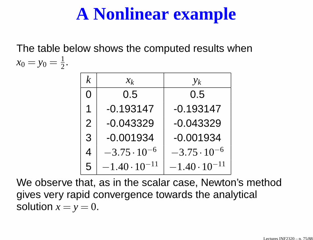
A Nonlinear example
The table below shows the computed results whenx0 = y0 = 1
2.
k xk yk
0 0.5 0.51 -0.193147 -0.1931472 -0.043329 -0.0433293 -0.001934 -0.0019344 −3.75·10−6 −3.75·10−6
5 −1.40·10−11 −1.40·10−11
We observe that, as in the scalar case, Newton’s methodgives very rapid convergence towards the analyticalsolution x = y = 0.
Lectures INF2320 – p. 75/88
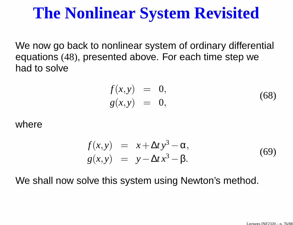
The Nonlinear System Revisited
We now go back to nonlinear system of ordinary differentialequations (48), presented above. For each time step wehad to solve
f (x,y) = 0,
g(x,y) = 0,(68)
where
f (x,y) = x+∆t y3−α,
g(x,y) = y−∆t x3−β.(69)
We shall now solve this system using Newton’s method.
Lectures INF2320 – p. 76/88
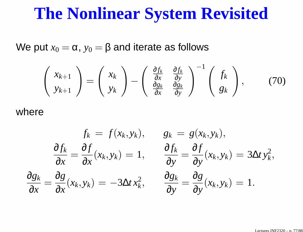
The Nonlinear System Revisited
We put x0 = α, y0 = β and iterate as follows
(
xk+1
yk+1
)
=
(
xk
yk
)
−(
∂ fk
∂x∂ fk
∂y∂gk
∂x∂gk
∂y
)−1(
fk
gk
)
, (70)
where
fk = f (xk,yk), gk = g(xk,yk),
∂ fk
∂x=
∂ f∂x
(xk,yk) = 1,∂ fk
∂y=
∂ f∂y
(xk,yk) = 3∆t y2k,
∂gk
∂x=
∂g∂x
(xk,yk) = −3∆t x2k,
∂gk
∂y=
∂g∂y
(xk,yk) = 1.
Lectures INF2320 – p. 77/88
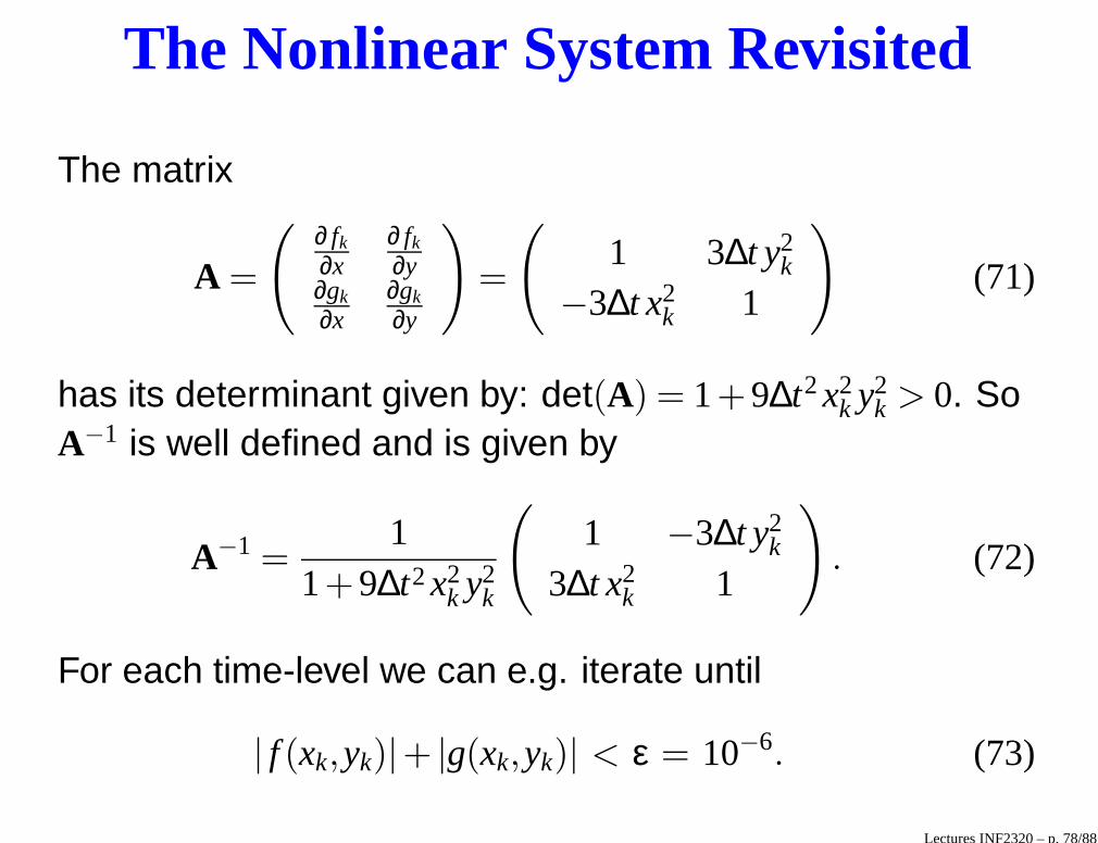
The Nonlinear System Revisited
The matrix
A =
(
∂ fk
∂x∂ fk
∂y∂gk
∂x∂gk
∂y
)
=
(
1 3∆t y2k
−3∆t x2k 1
)
(71)
has its determinant given by: det(A) = 1+9∆t2x2k y2
k > 0. SoA−1 is well defined and is given by
A−1 =1
1+9∆t2x2k y2
k
(
1 −3∆t y2k
3∆t x2k 1
)
. (72)
For each time-level we can e.g. iterate until
| f (xk,yk)|+ |g(xk,yk)| < ε = 10−6. (73)
Lectures INF2320 – p. 78/88
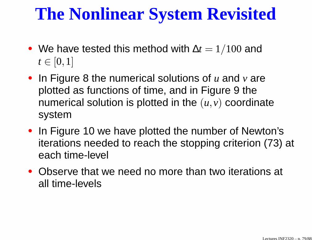
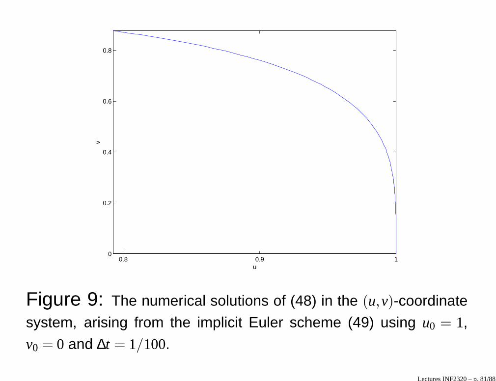
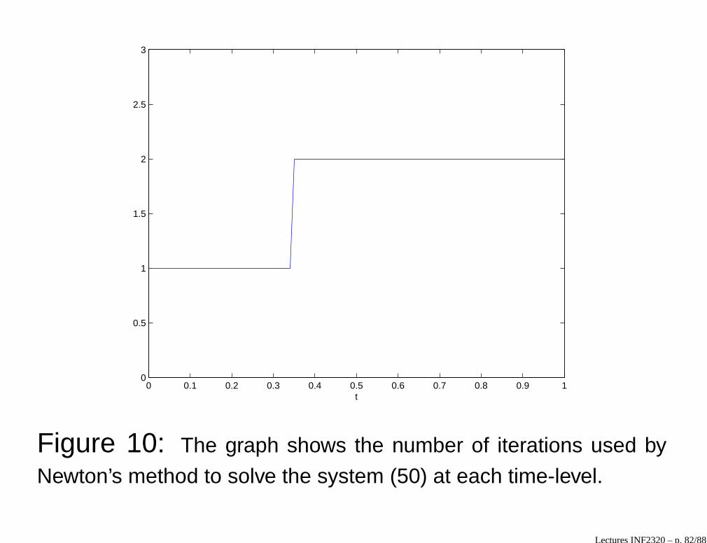
The Nonlinear System Revisited
• We have tested this method with ∆t = 1/100andt ∈ [0,1]
• In Figure 8 the numerical solutions of u and v areplotted as functions of time, and in Figure 9 thenumerical solution is plotted in the (u,v) coordinatesystem
• In Figure 10 we have plotted the number of Newton’siterations needed to reach the stopping criterion (73) ateach time-level
• Observe that we need no more than two iterations atall time-levels
Lectures INF2320 – p. 79/88
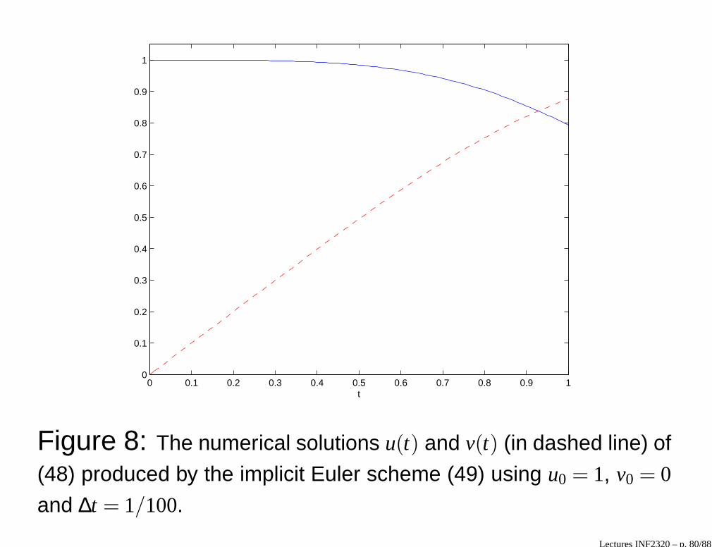
0 0.1 0.2 0.3 0.4 0.5 0.6 0.7 0.8 0.9 10
0.1
0.2
0.3
0.4
0.5
0.6
0.7
0.8
0.9
1
t
Figure 8: The numerical solutions u(t) and v(t) (in dashed line) of
(48) produced by the implicit Euler scheme (49) using u0 = 1, v0 = 0
and ∆t = 1/100.
Lectures INF2320 – p. 80/88
0.8 0.9 10
0.2
0.4
0.6
0.8
u
v
Figure 9: The numerical solutions of (48) in the (u,v)-coordinate
system, arising from the implicit Euler scheme (49) using u0 = 1,
v0 = 0 and ∆t = 1/100.
Lectures INF2320 – p. 81/88
0 0.1 0.2 0.3 0.4 0.5 0.6 0.7 0.8 0.9 10
0.5
1
1.5
2
2.5
3
t
Figure 10: The graph shows the number of iterations used by
Newton’s method to solve the system (50) at each time-level.
Lectures INF2320 – p. 82/88

Lectures INF2320 – p. 83/88

Lectures INF2320 – p. 84/88

Lectures INF2320 – p. 85/88

Lectures INF2320 – p. 86/88

Lectures INF2320 – p. 87/88

Lectures INF2320 – p. 88/88


![PDF - arxiv.org · PDF filearxiv:1712.03013v1 [math.ap] 8 dec 2017 uniqueness for neumann problems for nonlinear elliptic equations m.f. betta, o. guibe, and a. mercaldo´](https://static.fdocument.org/doc/165x107/5aaabbdf7f8b9a9a188e9b85/pdf-arxivorg-171203013v1-mathap-8-dec-2017-uniqueness-for-neumann-problems.jpg)
![arXiv:math/0703677v1 [math.AP] 22 Mar 2007arXiv:math/0703677v1 [math.AP] 22 Mar 2007 Ground state solutions for the nonlinear Schro¨dinger-Maxwell equations A. Azzollini ∗ & A.](https://static.fdocument.org/doc/165x107/60911ee4dabc19250f7c12a8/arxivmath0703677v1-mathap-22-mar-2007-arxivmath0703677v1-mathap-22-mar.jpg)