Nonequilibrium Molecular Dynamics Simulations of …rowley/publications/MD Publications...Draft...

Draft Date: October 5, 1999

Nonequilibrium Molecular Dynamics Simulations of Shear Viscosity:

Isoamyl Alcohol, n-Butyl Acetate and Their Mixtures

Y. Yang1, T. A. Pakkanen,2 and R. L. Rowley1,3

Draft Date: October 5, 1999

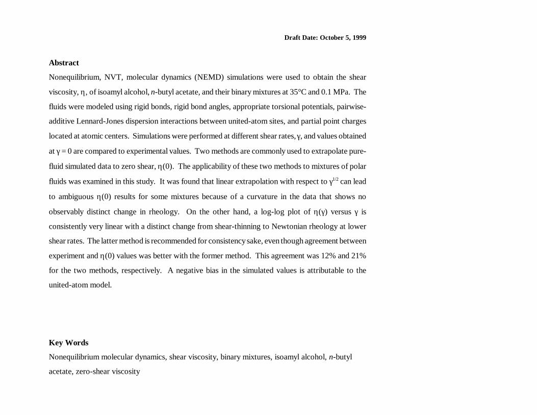
Abstract

Nonequilibrium, NVT, molecular dynamics (NEMD) simulations were used to obtain the shear

viscosity, η, of isoamyl alcohol, n-butyl acetate, and their binary mixtures at 35°C and 0.1 MPa. The

fluids were modeled using rigid bonds, rigid bond angles, appropriate torsional potentials, pairwise-

additive Lennard-Jones dispersion interactions between united-atom sites, and partial point charges

located at atomic centers. Simulations were performed at different shear rates, γ, and values obtained

at γ = 0 are compared to experimental values. Two methods are commonly used to extrapolate pure-

fluid simulated data to zero shear, η(0). The applicability of these two methods to mixtures of polar

fluids was examined in this study. It was found that linear extrapolation with respect to γ1/2 can lead

to ambiguous η(0) results for some mixtures because of a curvature in the data that shows no

observably distinct change in rheology. On the other hand, a log-log plot of η(γ) versus γ is

consistently very linear with a distinct change from shear-thinning to Newtonian rheology at lower

shear rates. The latter method is recommended for consistency sake, even though agreement between

experiment and η(0) values was better with the former method. This agreement was 12% and 21%

for the two methods, respectively. A negative bias in the simulated values is attributable to the

united-atom model.

Key Words

Nonequilibrium molecular dynamics, shear viscosity, binary mixtures, isoamyl alcohol, n-butyl

acetate, zero-shear viscosity

Yang, Pakkanen, & Rowley: NEMD Simulations...

1. INTRODUCTION

Accurate methods for predicting shear viscosity of a wide range of fluids and their mixtures are

not available. Although methods based on group contributions, corresponding states, significant

structure theory, and empirical correlations have had considerable success, none has adequately

captured the relationship between molecular structure and intermolecular interactions required to

produce an accurate predictive method for pure fluids and mixtures over a range of temperatures

and densities. Molecular simulations seem capable of providing this connection between

molecular structure and fluid viscosity. In particular, the accuracy of viscosity values obtained

from nonequilibrium molecular dynamics (NEMD) simulations is limited only by the efficacy of

the model(s) used to describe the geometry and intermolecular interactions and by the method

used to extrapolate simulated viscosities to zero shear. The simulations themselves accurately

account for all the physics underlying the relationship between fluid structure and the molecular

interactions for a given shear rate. Unfortunately, applied shear rates in NEMD simulations are

very large relative to those applied in experimental studies, and so some method of extrapolating

results from high shear rates to essentially zero shear is required for direct comparison of

simulated and experimental viscosities. The two issues of appropriate models and extrapolation

procedure are therefore key to development of NEMD simulations for use as predictive tools.

Considerable work has been done with regard to the first issue, the efficacy of various

intermolecular potential models, for certain types of fluids. Many NEMD simulations of n-alkanes


bonds or harmonic vibrational potentials. If rigid bonds are used, then bond lengths and angles are

fixed at their optimum locations as determined from experiment or ab initio geometry optimization.

To reduce the number of LJ interactions, hence the required simulation CPU time, -CHx groups are

often treated as a single, united-atom (UA) interacting site. Alternatively, hydrogen atoms are

explicitly included as separate interacting sites in all-atom (AA) models. Homogeneous UA models,

in which all -CHx sites are equivalent, have been shown to be reasonably accurate for simulating the

viscosity of n-alkanes; for example n-butane, n-decane, n-eicosane and n-hexadecane [1-4]. While

homogeneous UA models have also been used to simulate the viscosity of some branched and cyclic

molecules [5-7] such as isobutane, 5-butylnonane, tridecane, and cyclohexane, better accuracy is

generally obtained for such fluids when heterogeneous UA models are used. Such studies include

viscosity simulations for n-decane, n-hexadecane, n-tetracosane, 8-t-butyl-hexadecane, 6-methyl-

nonadecane, 3-methylhexane, and several others [8-11]. Simulated results for the viscosity of these

fluids are often in good quantitative agreement with experimental values, but there appears to be

considerable decay in the accuracy with increased branching [12].

For polar molecules, long-range Coulombic potentials must also be included in the

intermolecular model. This is commonly done using partial point charges located at atomic centers.

The Ewald sum method [13,14] is an accurate and efficient means of treating these long-range

interactions for small periodic systems. While potential truncation has also been used for polar fluids,

the cut-off contribution to the viscosity can be significant unless large systems are used [14]. There


Simulations of accurate viscosities of polar mixtures have only recently been conducted, and

then only for quite small molecules. However, results of such studies have been encouraging. For

example, very good agreement with experimental viscosities was obtained from simulations on binary

and ternary liquid mixtures of water, methanol and acetone [18]. Even though a standard combining

rule for the cross interactions was used, the simulated mixture viscosities exhibited maxima at the

appropriate compositions, and quantitative agreement with experimental values was very good. Most

of the error associated with those simulations was directly attributable to the inadequacy of the pure

water model.

With respect to the second issue, that of obtaining the NEMD value of the viscosity at low

enough shear for direct comparison to experiment, there is yet considerable debate on the appropriate

method for extrapolation to zero shear. Viscosities, η, are generally simulated at four or five shear

rates, γ, within a shear-thinning regime, and the resultant η(γ) values are extrapolated to γ = 0.

Unfortunately there is no known rigorous way to perform this extrapolation. Common practice has

been to plot η(γ) vs. γ1/2, which often results in linear behavior. However, more recent studies at

lower shear rates indicate that there may be a Newtonian region at very low shear rates from which

η(0) can be directly obtained as either the value at the lowest γ [10] or the average of several values

in the Newtonian region [18]. Unfortunately, the uncertainty in simulated values of η increases

exponentially at lower shear rates, and it is often difficult to distinguish with any degree of certainty


uij ' 4eij

s ij

rij

12

&s ij

rij

6

%qiqj

rij

(1)

butyl acetate (NBA), and their mixtures were obtained from NEMD simulations at 35°C and 0.1

MPa. The above-mentioned two extrapolation methods were used to obtain η(0) values for

comparison to experimental data. The purpose in so doing is twofold: to investigate the accuracy

of simulated viscosities using simple models for mixtures of branched, polar molecules and to

examine the applicability of these two extrapolation methods for mixtures of polar compounds. In

so doing, we have also extended previous work on mixtures of polar molecules to larger

molecules.

2. SIMULATION METHODOLOGY

2.1. Molecular Models

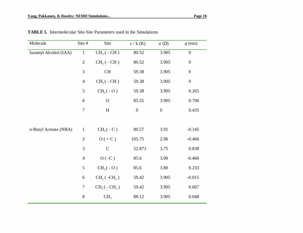
Heterogeneous, UA, pairwise-additive, site-site intermolecular potential models were used to model

intermolecular interactions. Pair interactions consisted of combined LJ and Coulombic interactions,

both located at atomic centers, in the form

All atoms except hydrogen atoms attached to carbon atoms were treated as interacting centers; -CHx

groups were treated within the UA framework, using different LJ parameters for different x

(heterogeneous UA). Model parameters used in this work are shown in Table I along with the site


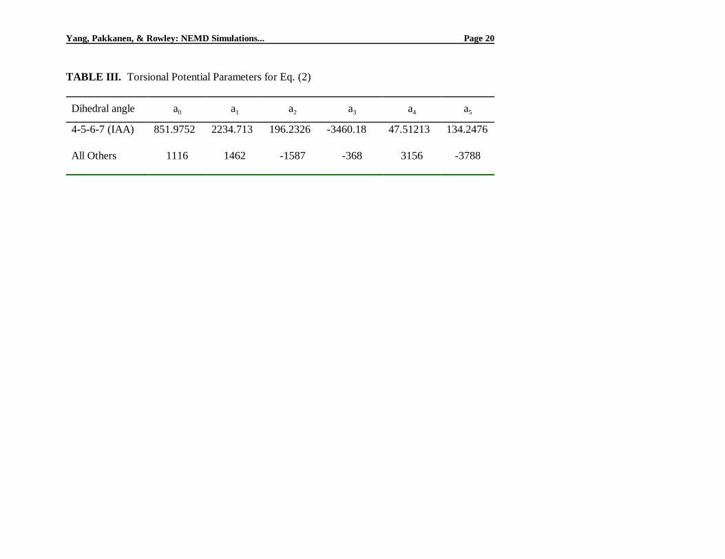
utors(f )/k ' j5

i'0ai cosif , (2)

calculated using the electrostatic potential method in Spartan®. Table II lists the optimized bond

distances and angles used.

The only intramolecualr potential to be included was the torsional potential, mathematically

represented by

where φ is the torsional angle and ai are coefficients in the cosine series shown. These latter

coefficients were obtained from the literature for dihedral angles associated with straight-chain groups

[6,22], but the ai for the branched portion of IAA (involving sites 4-5-6-7 as defined in Table I) were

regressed from energies of various configurations, calculated using the molecular mechanics model

MM2 in Hyperchem®. The resultant values of ai, as well as the values obtained from the literature,

are shown in Table III.

The repulsive part of the LJ potential (r-12) was truncated at r = 20 D , and long-range

corrections, though insignificant, were treated in the usual way (by calculating the property correction

from the cut-off to infinity with the radial distribution function set to unity). The attractive part of

the LJ potential (r-6) and the long-range Coulombic interactions were both handled using the Ewald

sum method. Details of this approach have been previously reported [18]. Cross LJ parameters (i

Ö j) were treated in the manner used by Wheeler and Rowley [18] in which a geometric mean is used


in the Ewald sum method.

2.2. Simulation Details

The NEMD simulations were performed using a NVT ensemble with a fourth-order correct predictor-

corrector numerical integration scheme. It employed the SLLOD equations of motion [21] in

combination with Lees-Edwards ‘sliding-brick’ boundary conditions to generate Couette flow.

Temperature was held constant using a Gaussian thermostat applied to molecular centers of mass.

Bond lengths and angles were fixed using Gaussian mechanics [22] to maintain a constant distance

between bonded sites and next-nearest neighbors.

Pure IAA, pure NBA, and nine mixture compositions were simulated using 300 molecules.

The time step for each simulation was chosen so that the root-mean-squared local displacement of

molecules was 0.7 pm per time step; it ranged from 2.38 to 2.73 fs. At each composition, a series

of NEMD simulation was performed at shear rates from 2 to 225 ps-1. All simulations utilized a

standard multiple-time-step algorithm [13] with six short steps per full step. Simulation lengths

ranged from 120 000 to 400 000 time-steps beyond equilibration. Equilibration duration depended

upon the starting configuration. Generally simulations were initiated from a lattice structure at a

lower density. During the equilibration portion of the simulation, the cell length was gradually

decreased until the density reached the desired value. Pure component densities at 1 atm and 35EC

were obtained from the DIPPR database [23] and the desired mixture densities were calculated using


? ' ?(0) & A? (3)

? ' ?(0) & A?2 (4)

? '?(0) Newtonian region

A?B shear&thinning region(7)

1?'

1?(0)

& A?1/2 (6)

? ' ?(0) & A?1/2 (5)

2.3. Viscosity at Zero Shear

As mentioned, one of the two objectives of this work was to examine the applicability of methods that

have been commonly used to obtain η(0) from η(γ) data for nonpolar, pure fluids to mixtures of polar

fluids. Because the previous methods are not based on rigorous theory, their applicability to mixtures

containing both polar interactions and branched molecular geometry is unclear. Previous studies on

nonpolar pure fluids have based the extrapolation of shear dependent viscosities to zero shear on one

of the following methods [3]

where γ is the applied shear rate. Equations (5) and (7) have emerged as the standard methods for


within the simulation. Generally this plateau is found by plotting η(γ) values on a log-log plot and

picking off the break point where the rheology changes between shear-thinning and Newtonian.

On the other hand, it has been observed that simulation results produce a straight line in the

shear-thinning region when plotted in accordance with Eq. (5), and that the extrapolated values are

often in good agreement with experimental data. Moreover, the results from Eq. (7) are often lower

than the those obtained from Eq. (5), so the extrapolation method does matter. Unfortunately, the

shear rate at which the Newtonian plateau occurs depends upon the molecule, and no general method

of predicting where it occurs exists, although Cummings et al. [10] have shown evidence that the

change in rheology may be related to the rotational relaxation time of the molecule. The systematic

occurrence of Newtonian plateaus in mixtures has not been investigated to our knowledge.

In this work, simulations were performed in the shear-thinning regime in order to investigate

the extrapolation capability of Eq. (5) for mixtures. Longer simulations were also performed at lower

shear rates in order to identify the Newtonian plateau in accordance with Eq. (7). A comparison of

the analysis methods was also performed, and simulation results from the two analysis methods were

compared to experimentally determined viscosities. In using Eq. (5), a weighted least squares

analysis was performed in order to find ?(0). Weights were computed from the variance of the η(γ)

data as determined from simple block averages of 10 000 time-steps each.

3. RESULTS


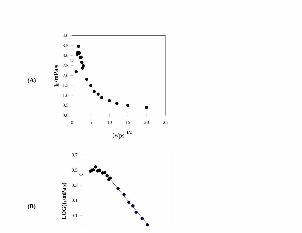
provide a unique value of η(0). Normally in analyzing η(γ) data in this manner, it is recognized that

the noise at low shear rates precludes their use in the data and that the shear-thinning rheology

changes back to Newtonian at even higher shear rates [1, 2]. Therefore, intermediate shear rates

would be probed, say 5 ps-1 # γ1/2 # 12 ps-1, and these would be used in conjunction with Eq. (5).

However, the data in Fig. 1(A) are not linear within the uncertainty of the data even in the 5 ps-1# γ1/2

# 12 ps-1 range. If the data within this range are analyzed using Eq. (5), the value of η(0) is very

close to the experimental one, but the agreement seems fortuitous and dependent upon the selected

points. It is clear that simulated viscosities for this fluid form a continuous curve rather than a

straight line when plotted against γ1/2. As can be seen in Fig. 1(B), a transition between the shear-

thinning and Newtonian regions around γ = 5 ps-1 can be identified. The η(0) value found in

accordance with Eq. (7) by using a weighted average of viscosities in the Newtonian region is 3.17

mPa·s, about 15% higher than the experimental value.

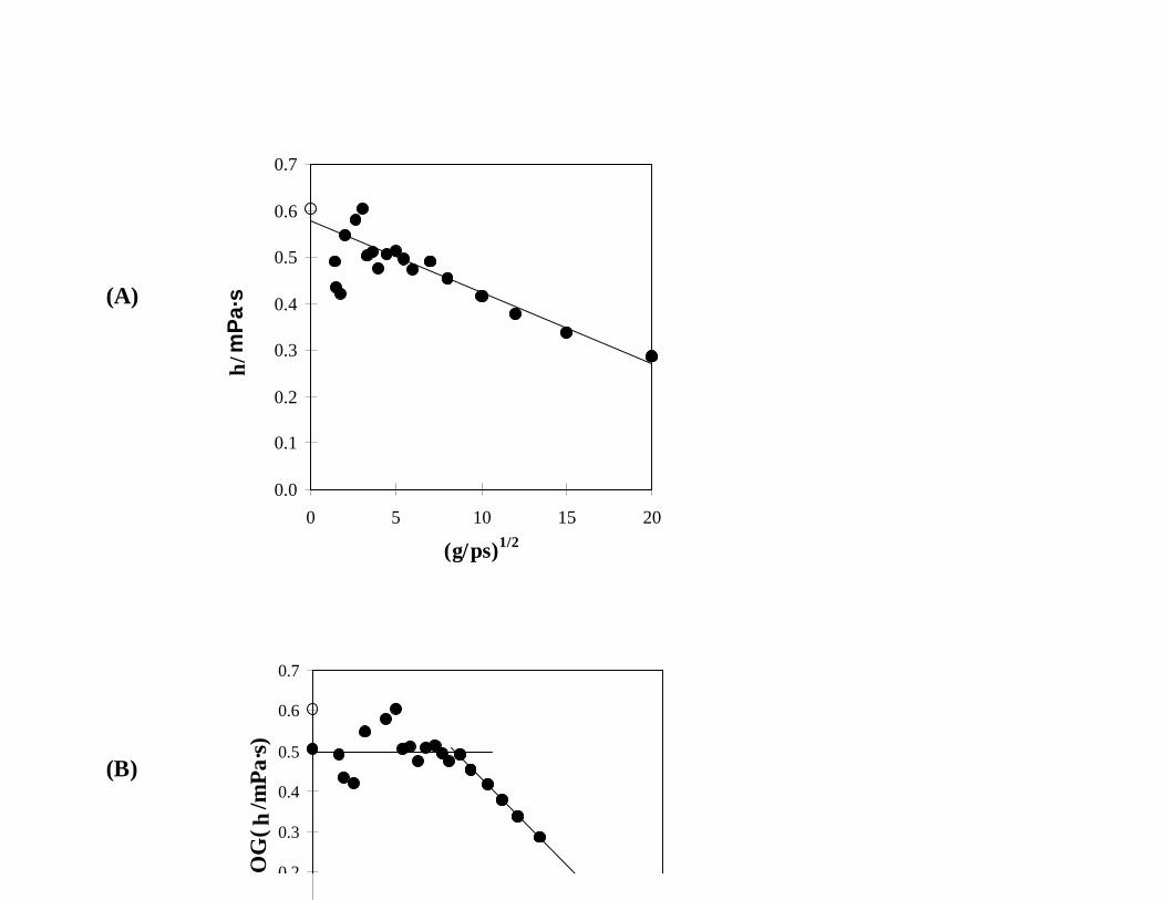
On the other hand, Fig. 2(A) shows that Eq. (5) describes η(γ) reasonably well for NBA and

does produce a value within 5% of the experimental value. There is still a slight curvature to the data,

but the linear correlation is much better than for IAA. Using Eq. (7) to analyze the data produces

a value for η(0) that is 18% lower than the experimental value, but the plateau appears to be rather

distinct at about 43 ps-1. While the disagreement between the experimental value and the η(0) value

is certainly attributable to inadequacies in the model (e.g., rigid bonds, UA assumption, and


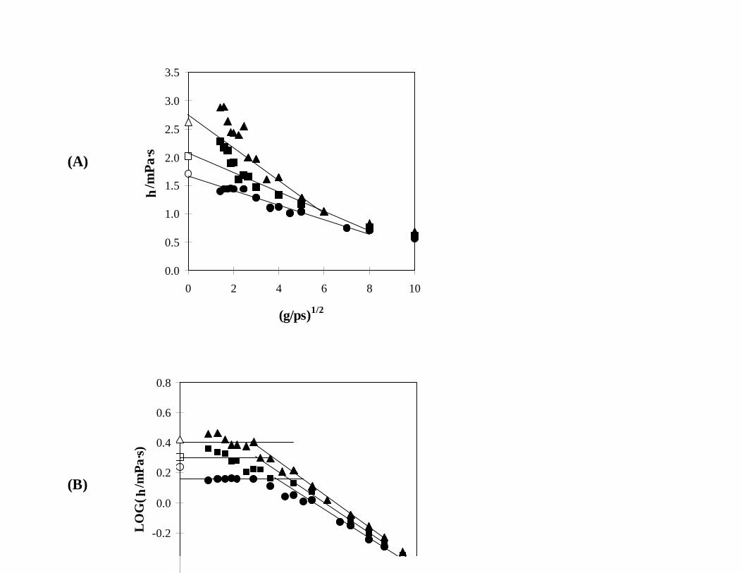
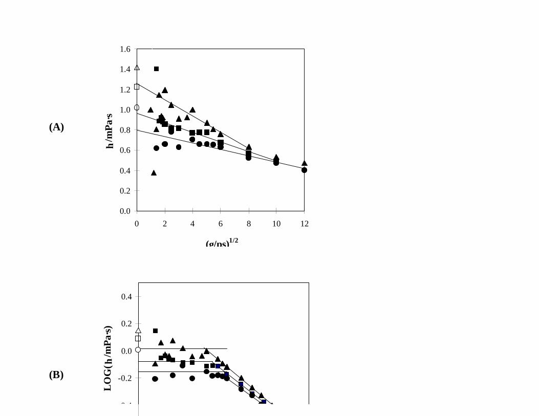
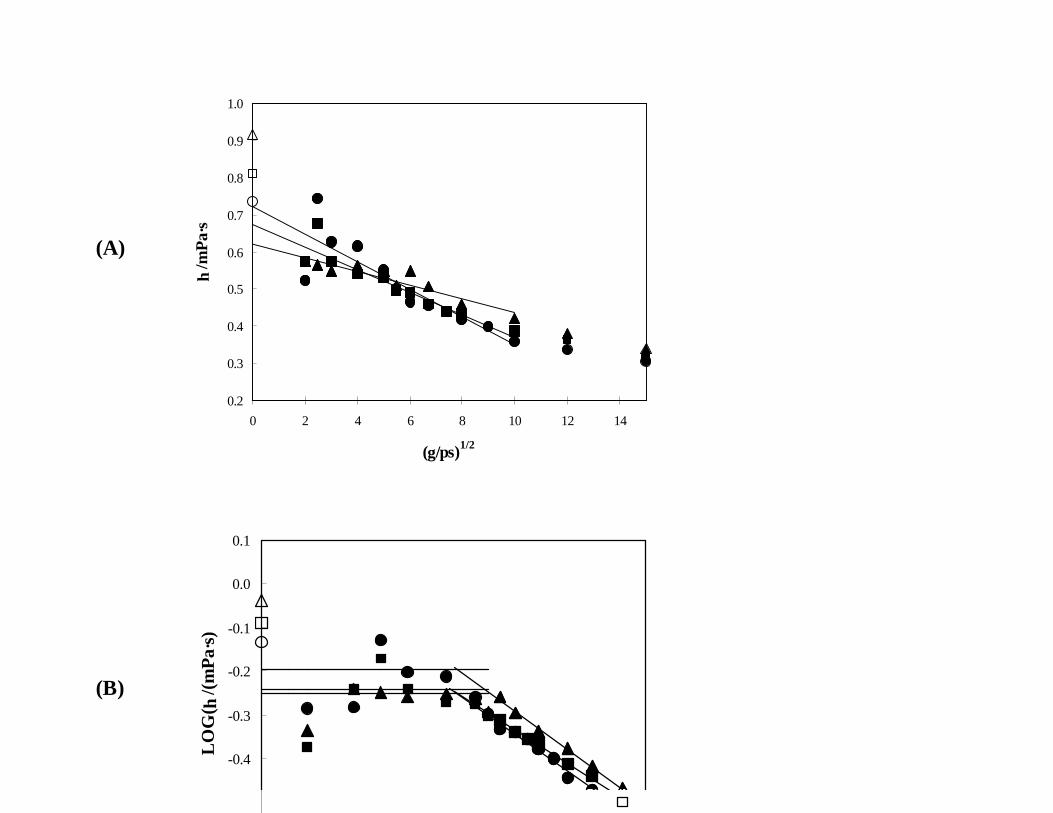
Figures 3 - 5 show the mixture results obtained from the simulations analyzed using Eqs. (5) and (7).

For the compositions rich in IAA, Fig. 3, the curvature of the simulated data observed for pure IAA

persists when Eq. (5) is used to extrapolate to zero shear. When the same data are analyzed in terms

of Eq. (7), definite breaks in the rheology are observed and the Newtonian viscosity can be obtained

in spite of the larger scatter at low γ. Both analyses produce reasonably good agreement with

experimental measurements. The results for mixtures that contain roughly equal molar amounts of

the two components, Fig. 4, appear to be more linear with respect to Eq. (5) than mixtures richer in

IAA, but it is difficult to tell where the linear region begins and ends. This makes the extrapolations

dependent upon the data chosen and the resultant η(0) value quite uncertain. When the data are

analyzed in accordance with Eq. (7) on a log-log plot, they become much more linear in the shear-

thinning region, and a definite transition to Newtonian behavior is observed at lower shear rates.

Both sets of extrapolated η(0) values appear to be lower than the experimental values. Finally, the

results for mixtures that are mostly NBA, Fig. 5, show considerable scatter even at higher shear rates

and are very difficult to analyze in terms of Eq. (5). The η(γ) data in Fig. 5(A) even exhibit what is

probably an unreal crossing behavior for the three different compositions, an artifact that is essentially

rectified when the data are plotted on a log-log plot. However, the viscosity plateaus that appear in

Fig. 5(B) are somewhat ambiguous due to the noise at the lower shear rates, and the η(0) values are

more difficult to obtain than at lower NBA compositions.


respectively.

4. CONCLUSIONS

Our results suggest that the most consistent extrapolation method for obtaining η(0) from NEMD

simulations is to perform enough long and large simulations in order to clearly identify the break in

η(γ) data at lower shear rates on a log-log plot. η(0) is then obtained in accordance with Eq. (7).

In the cases studied here, that of mixtures of polar fluids, a low-shear Newtonian plateau was

identifiable from the data when analyzed in this manner. The data in the shear-thinning region were

monotonic with respect to composition and more linear than when analyzed using Eq. (5). Analysis

using Eq. (5) leads to ambiguities in η(0) depending upon the range of γ used and in clearly

identifying a linear region over which the extrapolation is meaningful. Moreover, deviations from

linearity when using Eq. (5), curvature even in the shear-thinning regime, is dependent upon the

system and model structure.

While the simulated values at low shear where in better agreement with experimental data

when analyzed using Eq. (5) instead of Eq. (7), both methods showed considerable negative bias

indicating a systematic error due to inadequacies in the model. In a previous study of model effects

upon viscosity [12], it was found that rigid models produce slightly larger viscosities than models that

include potentials associated with vibrations and angle bending. The same study showed that UA

models under predict viscosities while AA models, explicitly including hydrogen atoms as interacting


viscosity data, still produces a negative bias for both analysis methods. It may be that results with

a more effective potential model would remove the bias observed here, making the viscosity plateau

method quantitatively more accurate in addition to being more consistent and theoretically justified.

ACKNOWLEDGEMENT

Support of this project by Neste Oil Company, Espoo, Finland, is gratefully acknowledged.


REFERENCES

[1] R. Edberg, G. P. Morriss, and D. J. Evans, J. Chem. Phys. 86:4555(1987).

[2] G. P. Morriss, P. J. Davis, and D. J. Evans, J. Chem. Phys. 94:7420 (1991).

[3] A. Berker, S. Chynoweth, U. C. Klomp and Y. Michopoulos, J. Chem. Soc. Faraday Trans.

88:1719 (1992).

[4] S. Chynoweth and Y. Michopoulos, Molec. Phys. 81:133 (1994).

[5] R. L. Rowley and J. F. Ely, Molec. Phys. 72:831 (1991).

[6] R. L. Rowley and J. F. Ely, Molec. Phys. 75:713 (1992).

[7] P. J. Daivis, D. J. Evans, and G. P. Morriss, J. Chem. Phys. 97:616 (1992).

[8] M. Lahtela, M. Linnolahti, T. A. Pakkanen, and R. L. Rowley, J. Chem. Phys. 108:2626

(1998).

[9] P. Padilla and S. Toxvaerd, J. Chem. Phys. 97:7687 (1992).

[10] S. T. Cui, S. A. Gupta, P. T. Cummings, and H. D. Cochran, J. Chem. Phys. 105:1214

(1996).

[11] M. Lahtela, T. A. Pakkanen, and R. L. Rowley, J. Phys. Chem. A 101:3449 (1997).

[12] W. Allen and R. L. Rowley, J. Chem. Phys. 106:10273 (1997).

[13] M. P. Allen and D. J. Tildesley, Computer simulation of liquids, (Clarendon, Oxford, 1987).

[14] D. R. Wheeler, N. G. Fuller, and R. L. Rowley, Molec. Phys. 92:55 (1997).

[15] P. T. Cummings and T. L. Varner, Jr., J. Chem. Phys. 89:6391 (1988).


[19] M. E. Van Leeuwen, Molec. Phys. 87:87 (1996).

[20] J. M. Brigs, T. B. Nguyen, and W. L. Jorgenesen, J. Phys. Chem. 95:3315 (1991).

[21] D. J. Evans and G. P. Morriss, Comput. Phys. Rep. 1:297 (1984).

[22] R. Edberg, D. J. Evans, and G. P. Morriss, J. Chem. Phys. 84:6933 (1986).

[23] DIPPR Chemical Database Web Version, http://dippr.byu.edu, 1999.

[24] M. Thayumanasundaram and P. B. Rao, J. Chem. Eng. Data. 16, 323 (1971).


Figure Captions

Fig. 1. Simulated viscosities (!) of IAA at 35EC and 0.1 MPa, analyzed using (A) Eq. (5) and (B)

Eq. (7) and compared to the experimental value (").

Fig. 2. Simulated viscosities (!) of NBA at 35EC and 0.1 MPa, analyzed using (A) Eq. (5) and (B)

Eq. (7) and compared to the experimental value (").

Fig. 3. Simulated viscosities of mixtures containing 10 mol% NBA + 90 mol% IAA (ï ), 20 mol%

NBA + 80 mol% IAA (#), and 30 mol% NBA + 70 mol% IAA (!) at 35EC and 0.1 MPa,

as analyzed using (A) Eq. (5) and (B) Eq. (7) and compared to the experimental values

(corresponding open symbols).










TABLE I. Intermolecular Site-Site Parameters used in the Simulations

Molecule Site # Site ε / k (K) σ (D ) q (esu)

Isoamyl Alcohol (IAA) 1 CH3 ( - CH ) 80.52 3.905 0

2 CH3 ( - CH ) 80.52 3.905 0

3 CH 59.38 3.905 0

4 CH2 ( - CH ) 59.38 3.905 0

5 CH2 ( - O ) 59.38 3.905 0.265

6 O 85.55 3.905 0.700

7 H 0 0 0.435

n-Butyl Acetate (NBA) 1 CH3 ( - C ) 80.57 3.91 -0.145

2 O ( = C ) 105.75 2.96 -0.466

3 C 52.873 3.75 0.838

4 O ( -C ) 85.6 3.00 -0.466

5 CH2 ( - O ) 85.6 3.80 0.233

6 CH2 ( -CH2 ) 59.42 3.905 -0.015

7 CH2 ( - CH3 ) 59.42 3.905 0.067

8 CH3 88.12 3.905 0.048


Table II. Model Bond Lengths and Angles

IAA bond distances (D )

1-3 1.546

0

2-3 1.546

0

3-4 1.551

2

4-5 1.551

7

5-6 1.435

3

6-7 0.991

3

IAA bond angles (degrees)

1-3-2 110.2

9

1-3-4 110.0

3

2-3-4 112.3

3

3-4-5 113.9

0

4-5-6 112.5

5

5-6-7 103.9

4

NBA bond distances (D )

1-3 1.538

9

2-3 1.215

7

3-4 1.393

3

4-5 1.440

2

5-6 1.545

1

6-7 1.544

4

7-8 1.540

8

NBA bond angles (degrees)

1-3-2 126.2 1-3-4 110.4 2-3-4 123.2 3-4-5 112.5


TABLE III. Torsional Potential Parameters for Eq. (2)

Dihedral angle a0 a1 a2 a3 a4 a5

4-5-6-7 (IAA) 851.9752 2234.713 196.2326 -3460.18 47.51213 134.2476

All Others 1116 1462 -1587 -368 3156 -3788


TABLE IV. η(0) Values Obtained using Eq. (5) and Eq. (10) in Comparison to Experimental Values

mole fraction

NBA

ρ/kmol·m-3 ηexp/mPa·s

[24]

η(0)/mPa·s

Eq. (5)

% Error

Eq. (5)

η(0)/mPa·s

Eq. (7)

% Error

Eq. (7)

0.0000 9.069 2.753 3.08 11.7 3.17 15.0

0.0998 8.915 2.631 2.75 4.4 2.51 -4.6

0.2003 8.753 2.091 2.08 -0.6 1.98 -5.2

0.3001 8.591 1.715 1.67 -2.9 1.44 -15.9

0.3999 8.430 1.418 1.26 -11.5 1.04 -26.9

0.4998 8.268 1.221 0.96 -21.3 0.84 -31.6

0.5999 8.107 1.079 0.78 -27.5 0.70 -34.8

0.6997 7.945 0.917 0.62 -32.2 0.56 -39.0

0.8002 7.783 0.811 0.68 -16.8 0.58 -29.0

0.9002 7.621 0.734 0.72 -1.6 0.64 -13.1

1.0000 7.452 0.604 0.58 -4.7 0.50 -17.9

0.0

0.5

1.0

1.5

2.0

2.5

3.0

3.5

4.0

0 5 10 15 20 25

(γ/ps)1/2

η/m

Pa·s

-0.1

0.1

0.3

0.5

0.7

LO

G( η

/mPa

·s)

(A)

(B)

0.0

0.1

0.2

0.3

0.4

0.5

0.6

0.7

0 5 10 15 20

(γ/ps)1/2

η/m

Pa·

s

0.2

0.3

0.4

0.5

0.6

0.7

LO

G( η

/mPa

·s)

(A)

(B)

0.0

0.5

1.0

1.5

2.0

2.5

3.0

3.5

0 2 4 6 8 10

(γ/ps)1/2

η/m

Pa·s

-0.2

0.0

0.2

0.4

0.6

0.8

LO

G( η

/mPa

·s)

(A)

(B)

0.0

0.2

0.4

0.6

0.8

1.0

1.2

1.4

1.6

0 2 4 6 8 10 12

(γ/ps)1/2

η/m

Pa·s

-0.4

-0.2

0.0

0.2

0.4

LO

G( η

/mPa

·s)

(A)

(B)

0.2

0.3

0.4

0.5

0.6

0.7

0.8

0.9

1.0

0 2 4 6 8 10 12 14

(γ/ps)1/2

η/m

Pa·s

-0.4

-0.3

-0.2

-0.1

0.0

0.1

LO

G( η

/(mPa

·s)

(A)

(B)

Nonequilibrium Molecular Dynamics Simulations of …rowley/publications/MD Publications...Draft...

Documents

Transcript of Nonequilibrium Molecular Dynamics Simulations of …rowley/publications/MD Publications...Draft...