Non-adiabatic Molecular Dynamics using Hefei-NAMDhome.ustc.edu.cn/~zqj/code/namd.pdf ·...
20
Non-adiabatic Molecular Dynamics using Hefei-NAMD Qijing Zheng Hefei National Laboratory for Physical Sciences at the Microscale University of Science and Technology of China Jun 10, 2018 Q.J. Zheng (HFNL USTC) Training Session Jun 10, 2018 1 / 17
Transcript of Non-adiabatic Molecular Dynamics using Hefei-NAMDhome.ustc.edu.cn/~zqj/code/namd.pdf ·...

Non-adiabatic Molecular Dynamics using Hefei-NAMD
Qijing Zheng
Hefei National Laboratory for Physical Sciences at the Microscale
University of Science and Technology of China
Jun 10, 2018
Q.J. Zheng (HFNL USTC) Training Session Jun 10, 2018 1 / 17
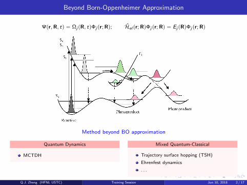
Beyond Born-Oppenheimer Approximation
Ψpr,R, tq “ Ωj pR, tqΦj pr;Rq; Hel pr;RqΦj pr;Rq “ Ej pRqΦj pr;Rq
Method beyond BO approximation
Quantum Dynamics
MCTDH
Mixed Quantum-Classical
Trajectory surface hopping (TSH)
Ehrenfest dynamics
. . .
Q.J. Zheng (HFNL USTC) Training Session Jun 10, 2018 2 / 17
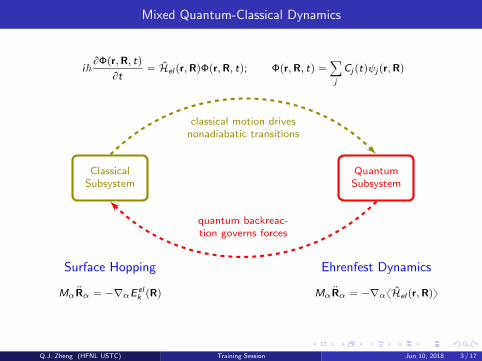
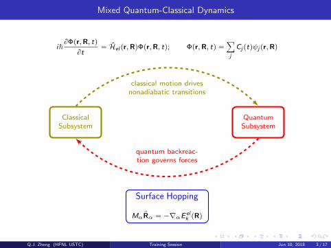
Mixed Quantum-Classical Dynamics
ClassicalSubsystem
QuantumSubsystem
i~BΦpr,R, tq
Bt“ Hel pr,RqΦpr,R, tq; Φpr,R, tq “
ÿ
j
Cj ptqψj pr,Rq
Surface Hopping
Mα:Rα “ ´∇αE el
k pRq
Ehrenfest Dynamics
Mα:Rα “ ´∇αxHel pr,Rqy
classical motion drivesnonadiabatic transitions
quantum backreac-tion governs forces
Q.J. Zheng (HFNL USTC) Training Session Jun 10, 2018 3 / 17
Mixed Quantum-Classical Dynamics
ClassicalSubsystem
QuantumSubsystem
i~BΦpr,R, tq
Bt“ Hel pr,RqΦpr,R, tq; Φpr,R, tq “
ÿ
j
Cj ptqψj pr,Rq
Surface Hopping
Mα:Rα “ ´∇αE el
k pRq
classical motion drivesnonadiabatic transitions
quantum backreac-tion governs forces
Q.J. Zheng (HFNL USTC) Training Session Jun 10, 2018 3 / 17
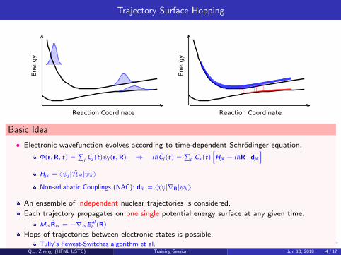
Trajectory Surface Hopping
Reaction Coordinate
Energ
y
Reaction Coordinate
Energ
y
Basic Idea
‚ Electronic wavefunction evolves according to time-dependent Schrodinger equation.
Φpr,R, tq “ř
j Cj ptqψj pr,Rq ñ i~ 9Cj ptq “ř
k Ckptq”
Hjk ´ i~ 9R ¨ djkı
Hjk “ xψj |Hel |ψky
Non-adiabatic Couplings (NAC): djk “ xψj |∇R|ψky
An ensemble of independent nuclear trajectories is considered.
Each trajectory propagates on one single potential energy surface at any given time.
Mα:Rα “ ´∇αE el
k pRq
Hops of trajectories between electronic states is possible.Tully’s Fewest-Switches algorithm et al.
Q.J. Zheng (HFNL USTC) Training Session Jun 10, 2018 4 / 17
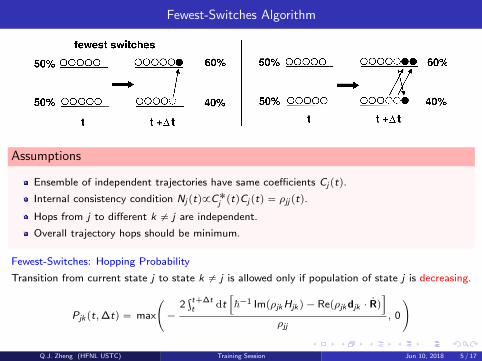
Fewest-Switches Algorithm
Assumptions
Ensemble of independent trajectories have same coefficients Cj ptq.
Internal consistency condition Nj ptq9C˚j ptqCj ptq “ ρjj ptq.
Hops from j to different k ‰ j are independent.
Overall trajectory hops should be minimum.
Fewest-Switches: Hopping Probability
Transition from current state j to state k ‰ j is allowed only if population of state j is decreasing.
Pjk pt,∆tq “ max
˜
´2şt`∆tt dt
”
~´1 ImpρjkHjk q ´ Repρjkdjk ¨ 9Rqı
ρjj, 0
¸
Q.J. Zheng (HFNL USTC) Training Session Jun 10, 2018 5 / 17

Fewest-Switches Algorithm
Assumptions
Ensemble of independent trajectories have same coefficients Cj ptq.
Internal consistency condition Nj ptq9C˚j ptqCj ptq “ ρjj ptq.
Hops from j to different k ‰ j are independent.
Overall trajectory hops should be minimum.
Fewest-Switches: Which state to hop
0 Pj1 Pj1 ` Pj2 Pj1 ` Pj2 ` Pj3 1. . .
k´1ÿ
l“1,l‰j
Pjl ă ξ ăkÿ
l“1,l‰j
Pjl then j Ñ k
Q.J. Zheng (HFNL USTC) Training Session Jun 10, 2018 5 / 17
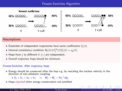
Fewest-Switches Algorithm
Assumptions
Ensemble of independent trajectories have same coefficients Cj ptq.
Internal consistency condition Nj ptq9C˚j ptqCj ptq “ ρjj ptq.
Hops from j to different k ‰ j are independent.
Overall trajectory hops should be minimum.
Fewest-Switches: After trajectory hops
Energy should be conserved after the hop e.g. by rescaling the nuclear velocity in thedirection of non-adiabatic coupling.
Ej `Kj “ Ek `Kk ñ Rkα “ Rj
α ´M´1α λdjk
Hops rejected when energy conservation not satisfied.
Q.J. Zheng (HFNL USTC) Training Session Jun 10, 2018 5 / 17
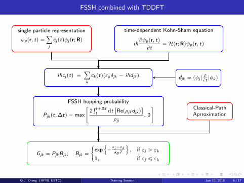
FSSH combined with TDDFT
single particle representation
ψppr, tq “ÿ
j
cj ptqφj pr;Rq
time-dependent Kohn-Sham equation
i~Bψppr, tq
Bt“ Hpr;Rqψppr, tq
i~ 9cj ptq “ÿ
k
ck ptqpεkδjk ´ i~djk q djk “ xφj |BBt|φky
FSSH hopping probability
Pjk pt,∆tq “ max
«
2şt`∆tt dt
“
Repρjkdjk q‰
ρjj, 0
ff Classical-PathAprroximation
Gjk “ PjkBjk ; Bjk “
#
exp!
´εj´εkkBT
)
, if εj ą εk
1, if εj ď εk
Q.J. Zheng (HFNL USTC) Training Session Jun 10, 2018 6 / 17
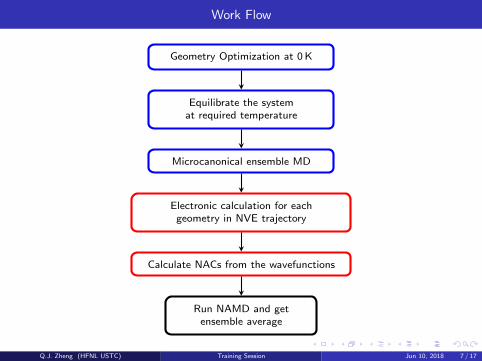
Work Flow
Geometry Optimization at 0 K
Equilibrate the systemat required temperature
Microcanonical ensemble MD
Electronic calculation for eachgeometry in NVE trajectory
Calculate NACs from the wavefunctions
Run NAMD and getensemble average
Q.J. Zheng (HFNL USTC) Training Session Jun 10, 2018 7 / 17
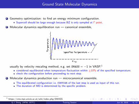
Ground State Molecular Dynamics
1 Geometry optimization: to find an energy minimum configuration.Supercell should be large enough because BZ is only sampled at Γ point.
2 Molecular dynamics equilibration run — canonical ensemble,
usually by velocity rescaling method, e.g. set SMASS “ ´1 in VASP.1
considered equilibrated when temperature fluctuation within ˘10% of the specified temperature.check the configuration before proceeding to next step.
3 Molecular dynamics production run — microcanonical ensemble.
The equilibrated configuration i.e. CONTCAR of the last step is used as input of this run.The duration of MD is determined by the specific problem.
1 https://cms.mpi.univie.ac.at/wiki/index.php/SMASS
Q.J. Zheng (HFNL USTC) Training Session Jun 10, 2018 8 / 17
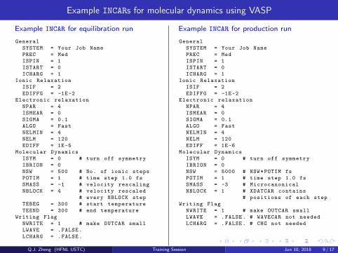
Example INCARs for molecular dynamics using VASP
Example INCAR for equilibration run
General
SYSTEM = Your Job Name
PREC = Med
ISPIN = 1
ISTART = 0
ICHARG = 1
Ionic Relaxation
ISIF = 2
EDIFFG = -1E-2
Electronic relaxation
NPAR = 4
ISMEAR = 0
SIGMA = 0.1
ALGO = Fast
NELMIN = 4
NELM = 120
EDIFF = 1E-5
Molecular Dynamics
ISYM = 0 # turn off symmetry
IBRION = 0
NSW = 500 # No. of ionic steps
POTIM = 1 # time step 1.0 fs
SMASS = -1 # velocity rescaling
NBLOCK = 4 # velocity rescaled
# every NBLOCK step
TEBEG = 300 # start temperature
TEEND = 300 # end temperature
Writing Flag
NWRITE = 1 # make OUTCAR small
LWAVE = .FALSE.
LCHARG = .FALSE.
Example INCAR for production run
General
SYSTEM = Your Job Name
PREC = Med
ISPIN = 1
ISTART = 0
ICHARG = 1
Ionic Relaxation
ISIF = 2
EDIFFG = -1E-2
Electronic relaxation
NPAR = 4
ISMEAR = 0
SIGMA = 0.1
ALGO = Fast
NELMIN = 4
NELM = 120
EDIFF = 1E-6
Molecular Dynamics
ISYM = 0 # turn off symmetry
IBRION = 0
NSW = 5000 # NSW*POTIM fs
POTIM = 1 # time step 1.0 fs
SMASS = -3 # Microcanonical
NBLOCK = 1 # XDATCAR contains
# positions of each step
Writing Flag
NWRITE = 1 # make OUTCAR small
LWAVE = .FALSE. # WAVECAR not needed
LCHARG = .FALSE. # CHG not needed
Q.J. Zheng (HFNL USTC) Training Session Jun 10, 2018 9 / 17
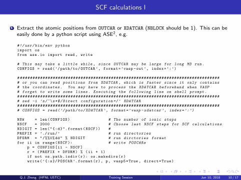
SCF calculations I
1 Extract the atomic positions from OUTCAR or XDATCAR (NBLOCK should be 1). This can beeasily done by a python script using ASE2, e.g.
#!/ usr/bin/env python
import os
from ase.io import read , write
# This may take a little while , since OUTCAR may be large for long MD run.
CONFIGS = read(’/path/to/OUTCAR ’, format=’vasp -out’, index=’:’)
# ###############################################################################
# or you can read positions from XDATCAR , which is faster since it only contains
# the coordinates . You may have to process the XDATCAR beforehand when VASP
# forget to write some lines. Executing the following line on shell prompt.
# ###############################################################################
# sed -i ’s/^\s*$/Direct configuration =/’ XDATCAR
# ###############################################################################
# CONFIGS = read (’/ path/to/XDATCAR ’, format=’vasp -xdatcar ’, index =’:’)
NSW = len(CONFIGS) # The number of ionic steps
NSCF = 2000 # Choose last NSCF steps for SCF calculations
NDIGIT = len(":d".format(NSCF)) #
PREFIX = ’./run/’ # run directories
DFORM = "/%%0%dd" % NDIGIT # run dirctories format
for ii in range(NSCF): # write POSCARs
p = CONFIGS[ii - NSCF]
r = (PREFIX + DFORM) % (ii + 1)
if not os.path.isdir(r): os.makedirs(r)
write(’:s/ POSCAR ’.format(r), p, vasp5=True , direct=True)
Q.J. Zheng (HFNL USTC) Training Session Jun 10, 2018 10 / 17
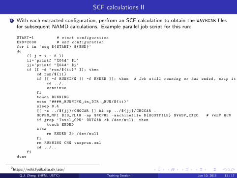
SCF calculations II
2 With each extracted configuration, perfrom an SCF calculation to obtain the WAVECAR filesfor subsequent NAMD calculations. Example parallel job script for this run:
START=1 # start configuration
END =2000 # end configuration
for i in ‘seq $START $END‘
do
(( j = i - 8 ))
ii=‘printf "%04d" $i‘
jj=‘printf "%04d" $j‘
if [[ -d "run/$ii" ]]; then
cd run/$ii
if [[ -f RUNNING || -f ENDED ]]; then # Job still running or has ended , skip it
cd ../..
continue
fi
touch RUNNING
echo "#### RUNNING in DIR: RUN/$ii"
sleep 0.4
[[ -s ../$jj/ CHGCAR ]] && cp ../$jj/ CHGCAR .
$OPEN_MPI $IB_FLAG -np $NCPUS -machinefile $HOSTFILE $VASP_EXEC # VASP RUN
if grep ’Total CPU’ OUTCAR >& /dev/null; then
touch ENDED
else
rm ENDED 2> /dev/null
fi
rm RUNNING CHG vasprun.xml
cd ../..
fi
done
2https://wiki.fysik.dtu.dk/ase/
Q.J. Zheng (HFNL USTC) Training Session Jun 10, 2018 11 / 17
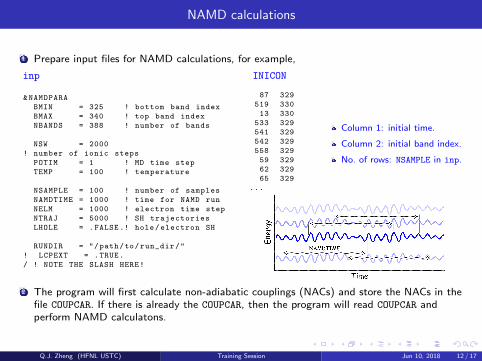
NAMD calculations
1 Prepare input files for NAMD calculations, for example,
inp
&NAMDPARA
BMIN = 325 ! bottom band index
BMAX = 340 ! top band index
NBANDS = 388 ! number of bands
NSW = 2000
! number of ionic steps
POTIM = 1 ! MD time step
TEMP = 100 ! temperature
NSAMPLE = 100 ! number of samples
NAMDTIME = 1000 ! time for NAMD run
NELM = 1000 ! electron time step
NTRAJ = 5000 ! SH trajectories
LHOLE = .FALSE.! hole/electron SH
RUNDIR = "/path/to/run_dir/"
! LCPEXT = .TRUE.
/ ! NOTE THE SLASH HERE!
INICON
87 329
519 330
13 330
533 329
541 329
542 329
558 329
59 329
62 329
65 329
...
Column 1: initial time.
Column 2: initial band index.
No. of rows: NSAMPLE in inp.
2 The program will first calculate non-adiabatic couplings (NACs) and store the NACs in thefile COUPCAR. If there is already the COUPCAR, then the program will read COUPCAR andperform NAMD calculatons.
Q.J. Zheng (HFNL USTC) Training Session Jun 10, 2018 12 / 17
Numerical evaluaton of NACs
The key quantity in the NAMD is the non-adiabatic couplings (NACs) and can be calculated byfinite difference method.
djk “ xφj |B
Bt|φky “ xφj |∇R|φky ¨ 9R
“xφj ptq|φk pt `∆tqy ´ xφj pt `∆tq|φk ptqy
2∆t(1)
φj ptq and φj pt `∆tq are Kohn-Sham (KS) pseudo-wavefunctions (WFC) from WAVECAR atdifferent time steps. Note that φj ptq are not orthonormalized for PAW PS.
For Gamma-only VASP, φj ptq are real functions. In addition, there is an arbitrary ˘1 phasefactor for each KS-WFC, which may affect the evaluaton of Eq. (1).
The inner product in the Eq. (1) can be obtained simply by summing over the products ofplain-wave coefficients3
xφj |φky “ÿ
G
c˚j pGq ¨ ck pGq (2)
3For Gamma-only WFCs, the plain-wave coefficients other G “ 0 are multiplied by a factor of?
2.
Q.J. Zheng (HFNL USTC) Training Session Jun 10, 2018 13 / 17
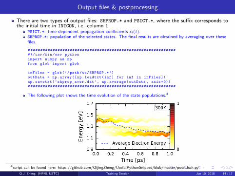
Output files & postprocessing
There are two types of output files: SHPROP.* and PSICT.*, where the suffix corresponds tothe initial time in INICON, i.e. column 1.
PSICT.*: time-dependent propagation coefficients ci ptq.SHPROP.*: population of the selected states. The final results are obtained by averaging over thesefiles.
# ###########################################################
#!/ usr/bin/env python
import numpy as np
from glob import glob
inFiles = glob(’/path/to/SHPROP .*’)
outData = np.array([np.loadtxt(inf) for inf in inFiles ])
np.savetxt(’shprop_aver.dat’, np.average(outData , axis =0))
# ###########################################################
The following plot shows the time evolution of the state populations.4
4script can be found here: https://github.com/QijingZheng/UsefulPythonSnippet/blob/master/poen fssh.py
Q.J. Zheng (HFNL USTC) Training Session Jun 10, 2018 14 / 17
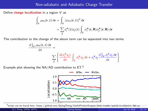
Non-adiabatic and Adiabatic Charge Transfer
Define charge localization in a region V asż
VρPEpr, tq dr “
ż
V|ψPEpr, tq|
2 dr
“ÿ
ij
c˚i ptqcj ptq
ż
Vφ˚i pr,Rqφ
˚j pr,Rqdr
The contribution to the change of the above term can be separated into two terms
dş
V ρPEpr, tq dr
dt“
ÿ
ij
#
dpc˚i cj q
dt
ż
Vφ˚i φj dr ` c˚i cj
dş
V φ˚i φj dr
dt
+
Example plot showing the NA/AD contribution to ET.5
5script can be found here: https://github.com/QijingZheng/UsefulPythonSnippet/blob/master/spatial localization fssh.py
Q.J. Zheng (HFNL USTC) Training Session Jun 10, 2018 15 / 17
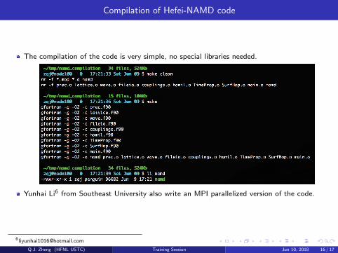
Compilation of Hefei-NAMD code
The compilation of the code is very simple, no special libraries needed.
Yunhai Li6 from Southeast University also write an MPI parallelized version of the code.
Q.J. Zheng (HFNL USTC) Training Session Jun 10, 2018 16 / 17

Thank you!