NEW ESTIMATES FOR THE BEURLING-AHLFORS...
28
NEW ESTIMATES FOR THE BEURLING-AHLFORS OPERATOR ON DIFFERENTIAL FORMS STEFANIE PETERMICHL † , LEONID SLAVIN ‡ , AND BRETT D. WICK * Abstract. We establish new p-estimates for the norm of the generalized Beurling– Ahlfors transform S acting on form-valued functions. Namely, we prove that S L p (R n ;Λ)→L p (R n ;Λ) ≤ n(p * - 1) where p * = max{p, p/(p - 1)}, thus extending the recent Nazarov–Volberg estimates to higher dimensions. The even-dimensional case has important implications for quasiconformal mappings. Some promising prospects for further improvement are discussed at the end. Contents Common notation 2 1. Introduction 2 2. Basic objects and main results 6 3. Estimates of the generalized Beurling–Ahlfors operator 13 4. The Bellman function proof of Theorem 2.3 16 5. Conclusion 25 Date : February 4, 2008. 2000 Mathematics Subject Classification. Primary 42BXX ; Secondary 42B15, 42B20. Key words and phrases. Beurling–Ahlfors Operator, Differential Forms, Heat Extensions, Bellman Functions. † Research supported in part by a National Science Foundation DMS grant. ‡ Research supported in part by a National Science Foundation DMS grant. * Research supported in part by a National Science Foundation DMS grant. 1
Transcript of NEW ESTIMATES FOR THE BEURLING-AHLFORS...
NEW ESTIMATES FOR THE BEURLING-AHLFORS OPERATORON DIFFERENTIAL FORMS
STEFANIE PETERMICHL†, LEONID SLAVIN‡, AND BRETT D. WICK∗
Abstract. We establish new p-estimates for the norm of the generalized Beurling–
Ahlfors transform S acting on form-valued functions. Namely, we prove that
‖S‖Lp(Rn;Λ)→Lp(Rn;Λ) ≤ n(p∗−1) where p∗ = maxp, p/(p−1), thus extending the
recent Nazarov–Volberg estimates to higher dimensions. The even-dimensional case
has important implications for quasiconformal mappings. Some promising prospects
for further improvement are discussed at the end.
Contents
Common notation 2
1. Introduction 2
2. Basic objects and main results 6
3. Estimates of the generalized Beurling–Ahlfors operator 13
4. The Bellman function proof of Theorem 2.3 16
5. Conclusion 25
Date: February 4, 2008.
2000 Mathematics Subject Classification. Primary 42BXX ; Secondary 42B15, 42B20.
Key words and phrases. Beurling–Ahlfors Operator, Differential Forms, Heat Extensions, Bellman
Functions.
† Research supported in part by a National Science Foundation DMS grant.
‡ Research supported in part by a National Science Foundation DMS grant.
∗ Research supported in part by a National Science Foundation DMS grant.1
2 S. PETERMICHL, L. SLAVIN, AND B. D. WICK
References 27
Common notation
:= equal by definition;
E a Hilbert space, fixed throughout;
〈·, ·〉E the inner product in E;
‖ · ‖E the norm on E induced by 〈·, ·〉E;
| · | either the absolute value or the Euclidean length in Rn,
clear from context;
∂i the partial derivative with respect to xi,∂
∂xi;
∂t the partial derivatives with respect to t, ∂∂t
;
C∞c (Rn;E) the space of infinitely differentiable compactly supported
E-valued functions on Rn;
Lp(Rn;E) the Lebesgue classes of E-valued functions on Rn.
1. Introduction
Singular integrals have historically played a very important role in the theory of
partial differential equations, for example in questions regarding the higher integra-
bility of weak solutions. In recent years the importance of computing or estimating
the the exact norms in Lp of singular integral operators has become clear. In this
light, it has been a long standing problem to find the exact operator norm of the
Beurling transform in scalar Lp.
3
The operator T : Lp(C) → Lp(C), defined by
T (f)(z) := − 1
π
∫C
f(w)
(w − z)2dA(w),
is called the (planar) Beurling–Ahlfors transform. This operator has the property
that it turns z-derivatives into z-derivatives: T(
∂f∂z
)= ∂f
∂z.
The long standing conjecture of T. Iwaniec [11] is that, for 1 < p <∞,
‖T ‖Lp(C)→Lp(C) = p∗ − 1,
where
p∗ = max
p,
p
p− 1
.
This problem has a long history, and has been reappearing in many papers on
regularity and integrability of quasiregular maps. Computing the exact norm of the
operator acting on Lp(C) is important, since estimates of the norm yield information
about the best integrability and minimal regularity of solutions to the Beltrami equa-
tion for example. A more detailed description of the benefit of finding these sharp
estimates can be found in [16] and the references therein.
The operator T is a Calderon–Zygmund operator, and so is bounded on all Lp(C),
but the standard methods of harmonic analysis fail to give good estimates of its norm.
In search for new, more efficient tools, sharp Burkholder inequalities for martingales
and the Bellman function technique have been shown to be very useful.
In 2000, F. Nazarov and A. Volberg, see [15], showed, using a special Bellman
function, that ‖T ‖p→p ≤ 2(p∗ − 1). Using martingale transforms, this result was
duplicated by Banuelos and Mendez-Hernandez [3]. Recently, using a more refined
4 S. PETERMICHL, L. SLAVIN, AND B. D. WICK
version of these methods, Banuelos and Janakiraman [1] were able to reduce the
constant 2 to approximately 1.575, the best known estimate to date.
There is a natural generalization of the planar Beurling–Ahlfors transform to dif-
ferential forms on Rn. Just as the planar operator T on the complex plane determines
many geometric and function-theoretic properties of quasiconformal mappings, esti-
mates for the generalized Beurling–Ahlfors operator S on forms have applications in
the theory of quasiregular mappings, where one computes the exponent of integrabil-
ity, the distortion of the Hausdorff dimension under the images of these mappings,
and the dimension of the removable singular set of the quasiregular map. These
important applications are a reason the operator S has drawn continued interest.
T. Iwaniec and G. Martin studied S in [12]. They developed a complex ‘method
of rotations’ to deal with the even kernel of the operator and showed that
‖S‖Lp(Rn;Λ)→Lp(Rn;Λ) ≤ (n+ 1)‖T ‖Lp(C)→Lp(C).
They also conjectured that
(1.1) ‖S‖Lp(Rn;Λ)→Lp(Rn;Λ) = (p∗ − 1).
It is well known that ‖S‖p→p ≥ (p∗ − 1), but the estimate from above has proved
elusive, just as it has in the planar case. Until now, the best known estimate was
due to Banuelos and Lindeman [2]. Using Burkholder-type inequalities for martingale
transforms, they showed that, under certain assumptions on n,
(1.2) ‖S‖Lp(Rn;Λ)→Lp(Rn;Λ) ≤ C(n)(p∗ − 1)
with C(n) = 43n− 2.
5
In this paper, we employ the line of reasoning developed by Petermichl and Volberg
in a weighted setting [16] and followed by Nazarov and Volberg in [15]. This line of
investigation has been further explored by Dragicevic and Volberg in [7–9]. This
reasoning produces good Lp → Lp estimates for any operator that can be represented
as a linear combination of products of two Riesz transforms. As such, the planar
Beurling–Ahlfors transform serves as a prime object of study. The estimates are by
duality: One recasts the action of the operator on two test functions in terms of
derivatives of their heat extensions:
∫Rm
(RkRjϕ)ψ = −2
∫∫Rm+1
+
∂kϕ∂jψ,
where f = f(x, t) is the heat extension of a function f. This new integral is estimated
using a Bellman function with appropriate size and concavity properties, together
with a Green’s function argument, which expresses the estimate in terms of the Lp
norms of the original test functions.
We are able to combine this approach with careful combinatorial considerations to
obtain new estimates on ‖S‖p→p. Specifically, with no restriction on n, we show that
‖S‖Lp(Rn;Λ)→Lp(Rn;Λ) ≤ n(p∗ − 1).
Although this result still falls far short from attaining the full Iwaniec–Martin con-
jecture, it improves significantly upon (1.2). In addition, we are hopeful that our
approach has the potential to yield a qualitative reduction in the size of C(n).
The structure of the paper is as follows. In Section 2, we describe the basic objects
under study, fix the notation to be used, and state the main results. In Section 3,
contingent on an “embedding-type” theorem, we prove an upper estimate for the
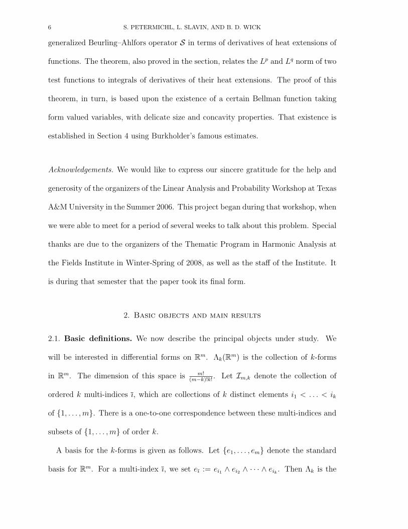
6 S. PETERMICHL, L. SLAVIN, AND B. D. WICK
generalized Beurling–Ahlfors operator S in terms of derivatives of heat extensions of
functions. The theorem, also proved in the section, relates the Lp and Lq norm of two
test functions to integrals of derivatives of their heat extensions. The proof of this
theorem, in turn, is based upon the existence of a certain Bellman function taking
form valued variables, with delicate size and concavity properties. That existence is
established in Section 4 using Burkholder’s famous estimates.
Acknowledgements. We would like to express our sincere gratitude for the help and
generosity of the organizers of the Linear Analysis and Probability Workshop at Texas
A&M University in the Summer 2006. This project began during that workshop, when
we were able to meet for a period of several weeks to talk about this problem. Special
thanks are due to the organizers of the Thematic Program in Harmonic Analysis at
the Fields Institute in Winter-Spring of 2008, as well as the staff of the Institute. It
is during that semester that the paper took its final form.
2. Basic objects and main results
2.1. Basic definitions. We now describe the principal objects under study. We
will be interested in differential forms on Rm. Λk(Rm) is the collection of k-forms
in Rm. The dimension of this space is m!(m−k)!k!
. Let Im,k denote the collection of
ordered k multi-indices ı, which are collections of k distinct elements i1 < . . . < ik
of 1, . . . ,m. There is a one-to-one correspondence between these multi-indices and
subsets of 1, . . . ,m of order k.
A basis for the k-forms is given as follows. Let e1, . . . , em denote the standard
basis for Rm. For a multi-index ı, we set eı := ei1 ∧ ei2 ∧ · · · ∧ eik . Then Λk is the
7
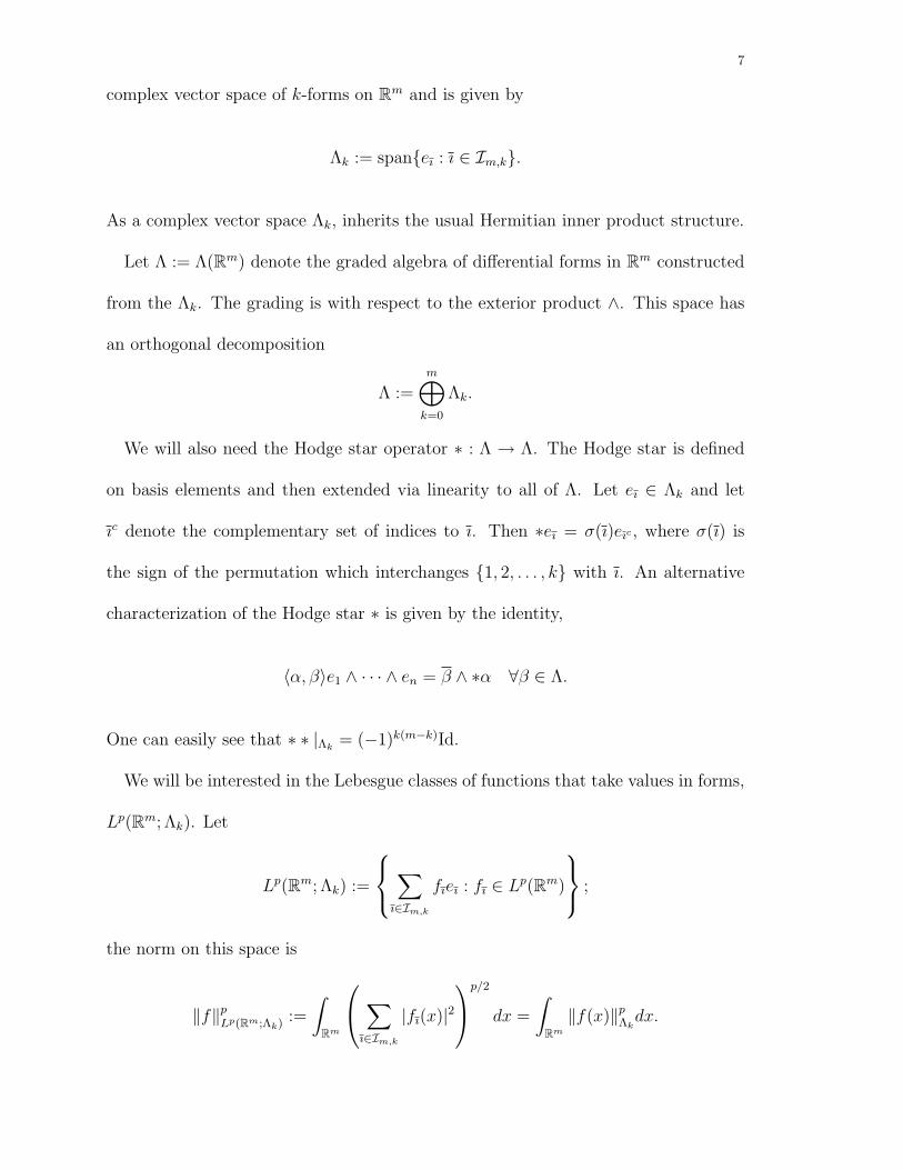
complex vector space of k-forms on Rm and is given by
Λk := spaneı : ı ∈ Im,k.
As a complex vector space Λk, inherits the usual Hermitian inner product structure.
Let Λ := Λ(Rm) denote the graded algebra of differential forms in Rm constructed
from the Λk. The grading is with respect to the exterior product ∧. This space has
an orthogonal decomposition
Λ :=m⊕
k=0
Λk.
We will also need the Hodge star operator ∗ : Λ → Λ. The Hodge star is defined
on basis elements and then extended via linearity to all of Λ. Let eı ∈ Λk and let
ıc denote the complementary set of indices to ı. Then ∗eı = σ(ı)eıc , where σ(ı) is
the sign of the permutation which interchanges 1, 2, . . . , k with ı. An alternative
characterization of the Hodge star ∗ is given by the identity,
〈α, β〉e1 ∧ · · · ∧ en = β ∧ ∗α ∀β ∈ Λ.
One can easily see that ∗ ∗ |Λk= (−1)k(m−k)Id.
We will be interested in the Lebesgue classes of functions that take values in forms,
Lp(Rm; Λk). Let
Lp(Rm; Λk) :=
∑ı∈Im,k
fıeı : fı ∈ Lp(Rm)
;
the norm on this space is
‖f‖pLp(Rm;Λk) :=
∫Rm
∑ı∈Im,k
|fı(x)|2p/2
dx =
∫Rm
‖f(x)‖pΛkdx.
8 S. PETERMICHL, L. SLAVIN, AND B. D. WICK
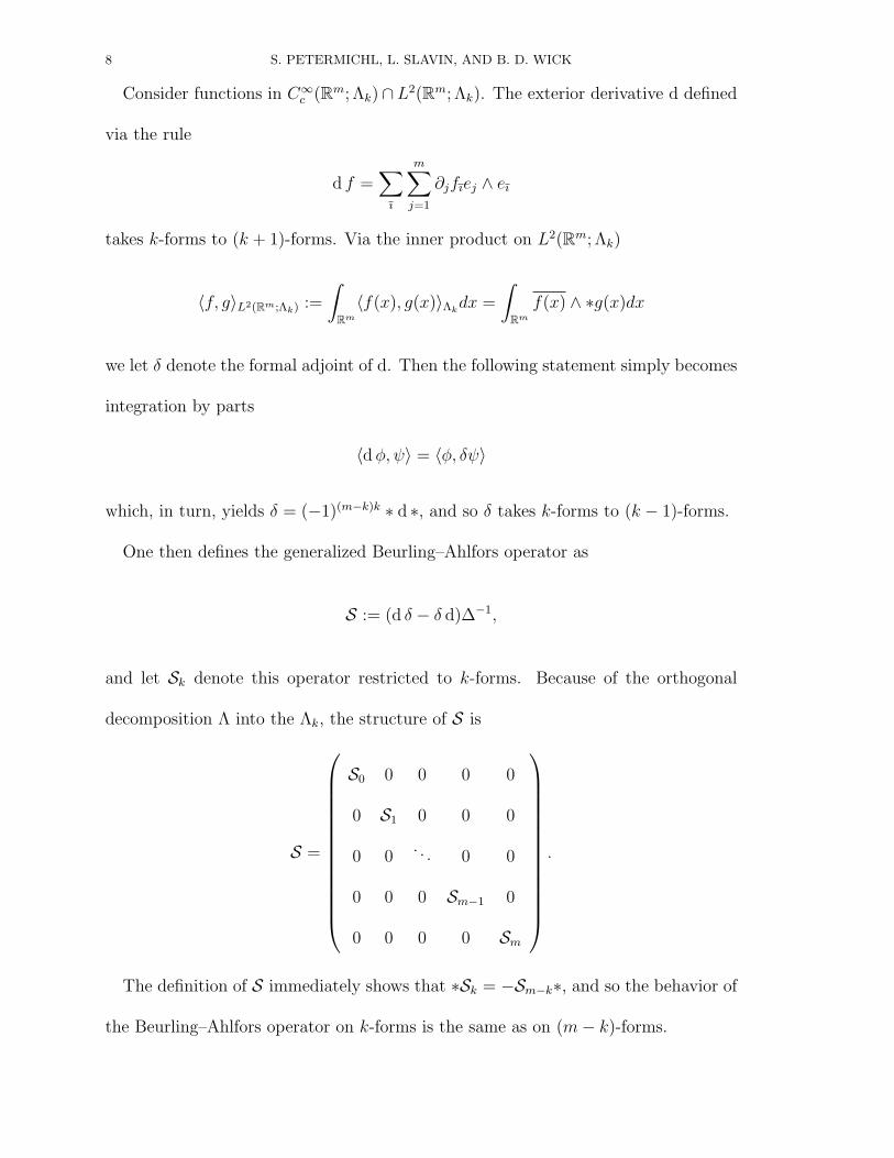
Consider functions in C∞c (Rm; Λk)∩L2(Rm; Λk). The exterior derivative d defined
via the rule
d f =∑
ı
m∑j=1
∂jfıej ∧ eı
takes k-forms to (k + 1)-forms. Via the inner product on L2(Rm; Λk)
〈f, g〉L2(Rm;Λk) :=
∫Rm
〈f(x), g(x)〉Λkdx =
∫Rm
f(x) ∧ ∗g(x)dx
we let δ denote the formal adjoint of d. Then the following statement simply becomes
integration by parts
〈dφ, ψ〉 = 〈φ, δψ〉
which, in turn, yields δ = (−1)(m−k)k ∗ d ∗, and so δ takes k-forms to (k − 1)-forms.
One then defines the generalized Beurling–Ahlfors operator as
S := (d δ − δ d)∆−1,
and let Sk denote this operator restricted to k-forms. Because of the orthogonal
decomposition Λ into the Λk, the structure of S is
S =
S0 0 0 0 0
0 S1 0 0 0
0 0. . . 0 0
0 0 0 Sm−1 0
0 0 0 0 Sm
.
The definition of S immediately shows that ∗Sk = −Sm−k∗, and so the behavior of
the Beurling–Ahlfors operator on k-forms is the same as on (m− k)-forms.
9
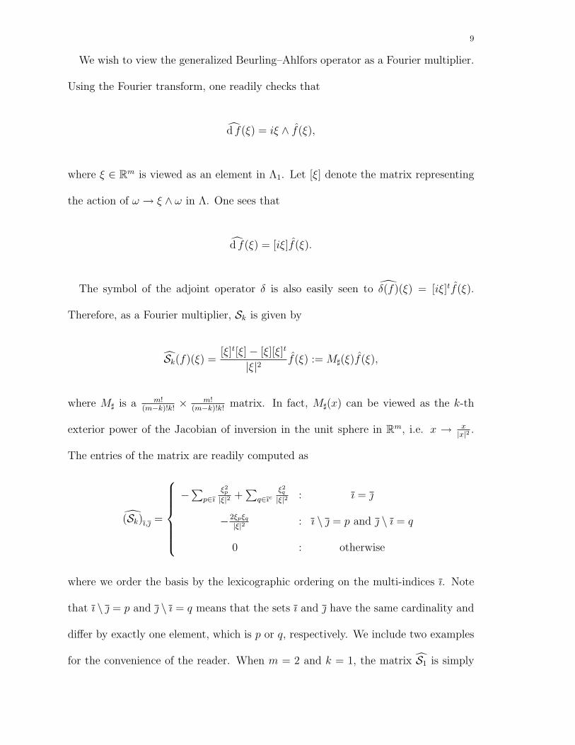
We wish to view the generalized Beurling–Ahlfors operator as a Fourier multiplier.
Using the Fourier transform, one readily checks that
d f(ξ) = iξ ∧ f(ξ),
where ξ ∈ Rm is viewed as an element in Λ1. Let [ξ] denote the matrix representing
the action of ω → ξ ∧ ω in Λ. One sees that
d f(ξ) = [iξ]f(ξ).
The symbol of the adjoint operator δ is also easily seen to δ(f)(ξ) = [iξ]tf(ξ).
Therefore, as a Fourier multiplier, Sk is given by
Sk(f)(ξ) =[ξ]t[ξ]− [ξ][ξ]t
|ξ|2f(ξ) := M](ξ)f(ξ),
where M] is a m!(m−k)!k!
× m!(m−k)!k!
matrix. In fact, M](x) can be viewed as the k-th
exterior power of the Jacobian of inversion in the unit sphere in Rm, i.e. x → x|x|2 .
The entries of the matrix are readily computed as
(Sk)ı, =
−∑
p∈ı
ξ2p
|ξ|2 +∑
q∈ıcξ2q
|ξ|2 : ı =
−2ξpξq
|ξ|2 : ı \ = p and \ ı = q
0 : otherwise
where we order the basis by the lexicographic ordering on the multi-indices ı. Note
that ı \ = p and \ ı = q means that the sets ı and have the same cardinality and
differ by exactly one element, which is p or q, respectively. We include two examples
for the convenience of the reader. When m = 2 and k = 1, the matrix S1 is simply
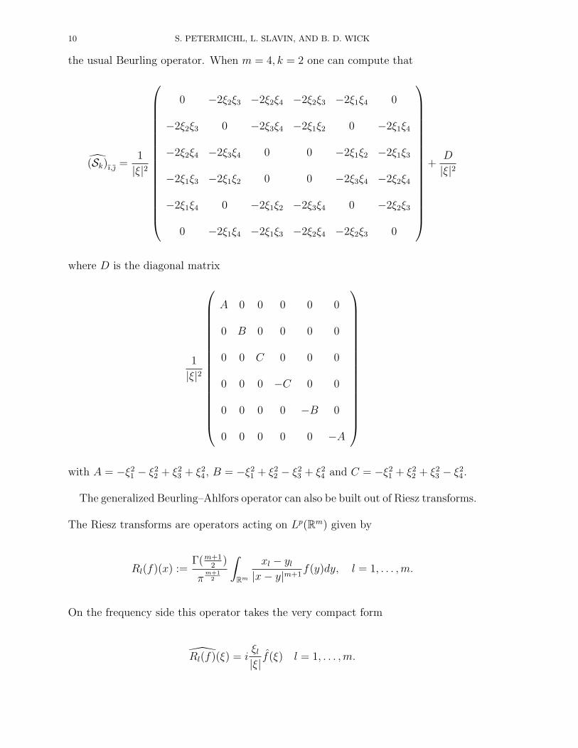
10 S. PETERMICHL, L. SLAVIN, AND B. D. WICK
the usual Beurling operator. When m = 4, k = 2 one can compute that
(Sk)ı, =1
|ξ|2
0 −2ξ2ξ3 −2ξ2ξ4 −2ξ2ξ3 −2ξ1ξ4 0
−2ξ2ξ3 0 −2ξ3ξ4 −2ξ1ξ2 0 −2ξ1ξ4
−2ξ2ξ4 −2ξ3ξ4 0 0 −2ξ1ξ2 −2ξ1ξ3
−2ξ1ξ3 −2ξ1ξ2 0 0 −2ξ3ξ4 −2ξ2ξ4
−2ξ1ξ4 0 −2ξ1ξ2 −2ξ3ξ4 0 −2ξ2ξ3
0 −2ξ1ξ4 −2ξ1ξ3 −2ξ2ξ4 −2ξ2ξ3 0
+D
|ξ|2
where D is the diagonal matrix
1
|ξ|2
A 0 0 0 0 0
0 B 0 0 0 0
0 0 C 0 0 0
0 0 0 −C 0 0
0 0 0 0 −B 0
0 0 0 0 0 −A
with A = −ξ2
1 − ξ22 + ξ2
3 + ξ24 , B = −ξ2
1 + ξ22 − ξ2
3 + ξ24 and C = −ξ2
1 + ξ22 + ξ2
3 − ξ24 .
The generalized Beurling–Ahlfors operator can also be built out of Riesz transforms.
The Riesz transforms are operators acting on Lp(Rm) given by
Rl(f)(x) :=Γ(m+1
2)
πm+1
2
∫Rm
xl − yl
|x− y|m+1f(y)dy, l = 1, . . . ,m.
On the frequency side this operator takes the very compact form
Rl(f)(ξ) = iξl|ξ|f(ξ) l = 1, . . . ,m.
11
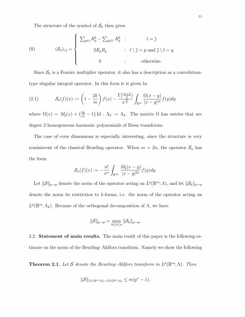
The structure of the symbol of Sk then gives
(S) (Sk)ı, =
∑p∈ıR
2p −
∑q∈ıc R
2q : ı =
2RpRq : ı \ = p and \ ı = q
0 : otherwise.
Since Sk is a Fourier multiplier operator, it also has a description as a convolution-
type singular integral operator. In this form it is given by
(2.1) Sk(f)(x) :=
(1− 2k
m
)f(x)−
Γ(m+22
)
πm2
∫Rm
Ω(x− y)
|x− y|mf(y)dy
where Ω(x) = M](x) +(
2km− 1)Id : Λk → Λk. The matrix Ω has entries that are
degree 2 homogeneous harmonic polynomials of Riesz transforms.
The case of even dimensions is especially interesting, since the structure is very
reminiscent of the classical Beurling operator. When m = 2n, the operator Sn has
the form
Sn(f)(x) := − n!
πn
∫R2n
M](x− y)
|x− y|2nf(y)dy.
Let ‖S‖p→p denote the norm of the operator acting on Lp(Rm; Λ), and let ‖Sk‖p→p
denote the norm its restriction to k-forms, i.e. the norm of the operator acting on
Lp(Rm; Λk). Because of the orthogonal decomposition of Λ, we have
‖S‖p→p = max0≤k≤n
‖Sk‖p→p.
2.2. Statement of main results. The main result of this paper is the following es-
timate on the norm of the Beurling–Ahlfors transform. Namely we show the following
Theorem 2.1. Let S denote the Beurling–Ahlfors transform in Lp(Rm; Λ). Then
‖S‖Lp(Rm;Λ)→Lp(Rm;Λ) ≤ m(p∗ − 1).
12 S. PETERMICHL, L. SLAVIN, AND B. D. WICK
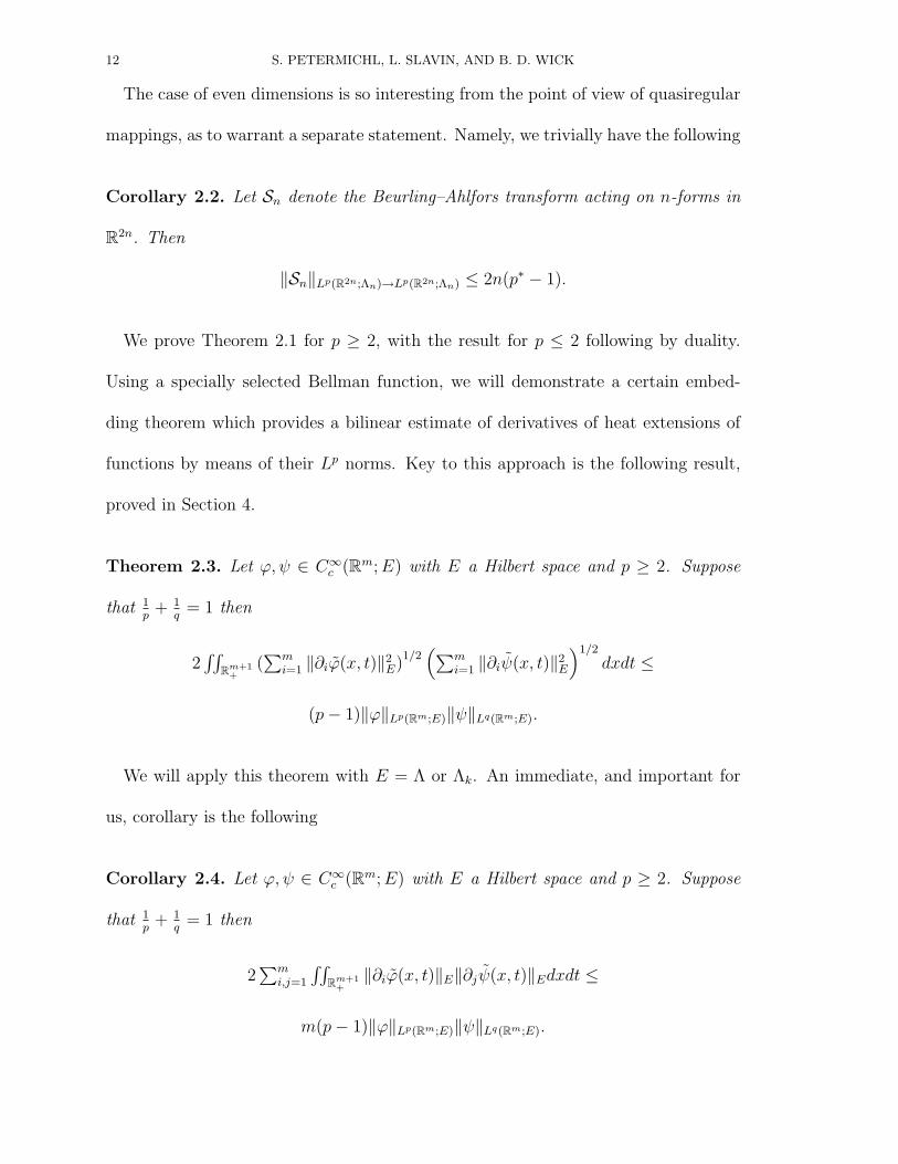
The case of even dimensions is so interesting from the point of view of quasiregular
mappings, as to warrant a separate statement. Namely, we trivially have the following
Corollary 2.2. Let Sn denote the Beurling–Ahlfors transform acting on n-forms in
R2n. Then
‖Sn‖Lp(R2n;Λn)→Lp(R2n;Λn) ≤ 2n(p∗ − 1).
We prove Theorem 2.1 for p ≥ 2, with the result for p ≤ 2 following by duality.
Using a specially selected Bellman function, we will demonstrate a certain embed-
ding theorem which provides a bilinear estimate of derivatives of heat extensions of
functions by means of their Lp norms. Key to this approach is the following result,
proved in Section 4.
Theorem 2.3. Let ϕ, ψ ∈ C∞c (Rm;E) with E a Hilbert space and p ≥ 2. Suppose
that 1p
+ 1q
= 1 then
2∫∫
Rm+1+
(∑m
i=1 ‖∂iϕ(x, t)‖2E)
1/2(∑m
i=1 ‖∂iψ(x, t)‖2E
)1/2
dxdt ≤
(p− 1)‖ϕ‖Lp(Rm;E)‖ψ‖Lq(Rm;E).
We will apply this theorem with E = Λ or Λk. An immediate, and important for
us, corollary is the following
Corollary 2.4. Let ϕ, ψ ∈ C∞c (Rm;E) with E a Hilbert space and p ≥ 2. Suppose
that 1p
+ 1q
= 1 then
2∑m
i,j=1
∫∫Rm+1
+‖∂iϕ(x, t)‖E‖∂jψ(x, t)‖Edxdt ≤
m(p− 1)‖ϕ‖Lp(Rm;E)‖ψ‖Lq(Rm;E).
13
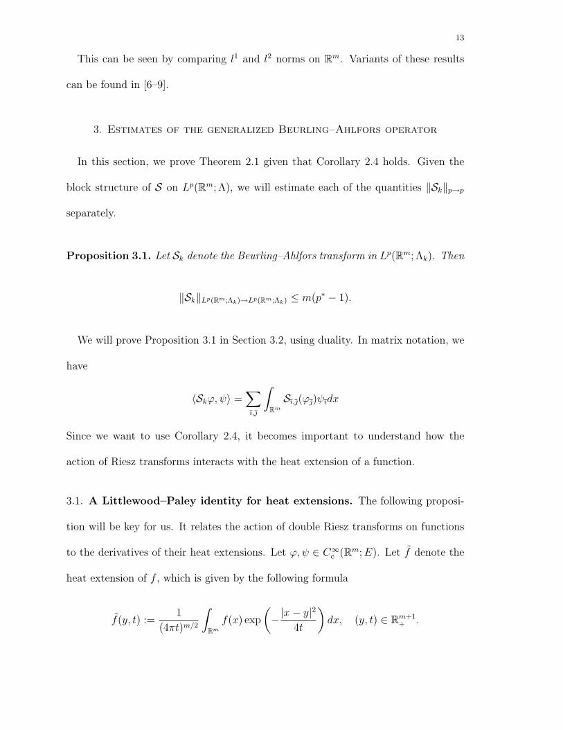
This can be seen by comparing l1 and l2 norms on Rm. Variants of these results
can be found in [6–9].
3. Estimates of the generalized Beurling–Ahlfors operator
In this section, we prove Theorem 2.1 given that Corollary 2.4 holds. Given the
block structure of S on Lp(Rm; Λ), we will estimate each of the quantities ‖Sk‖p→p
separately.
Proposition 3.1. Let Sk denote the Beurling–Ahlfors transform in Lp(Rm; Λk). Then
‖Sk‖Lp(Rm;Λk)→Lp(Rm;Λk) ≤ m(p∗ − 1).
We will prove Proposition 3.1 in Section 3.2, using duality. In matrix notation, we
have
〈Skϕ, ψ〉 =∑ı,
∫Rm
Sı,(ϕ)ψıdx
Since we want to use Corollary 2.4, it becomes important to understand how the
action of Riesz transforms interacts with the heat extension of a function.
3.1. A Littlewood–Paley identity for heat extensions. The following proposi-
tion will be key for us. It relates the action of double Riesz transforms on functions
to the derivatives of their heat extensions. Let ϕ, ψ ∈ C∞c (Rm;E). Let f denote the
heat extension of f , which is given by the following formula
f(y, t) :=1
(4πt)m/2
∫Rm
f(x) exp
(−|x− y|2
4t
)dx, (y, t) ∈ Rm+1
+ .
14 S. PETERMICHL, L. SLAVIN, AND B. D. WICK
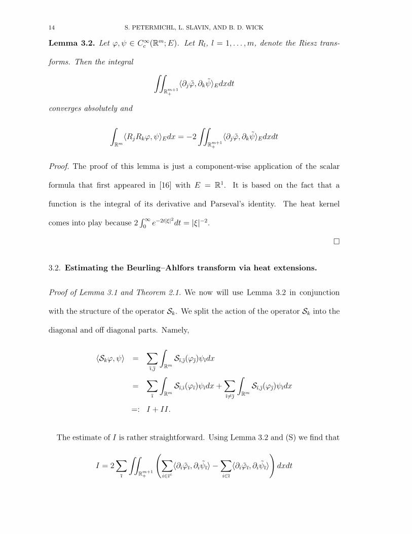
Lemma 3.2. Let ϕ, ψ ∈ C∞c (Rm;E). Let Rl, l = 1, . . . ,m, denote the Riesz trans-
forms. Then the integral ∫∫Rm+1
+
〈∂jϕ, ∂kψ〉Edxdt
converges absolutely and
∫Rm
〈RjRkϕ, ψ〉Edx = −2
∫∫Rm+1
+
〈∂jϕ, ∂kψ〉Edxdt
Proof. The proof of this lemma is just a component-wise application of the scalar
formula that first appeared in [16] with E = R1. It is based on the fact that a
function is the integral of its derivative and Parseval’s identity. The heat kernel
comes into play because 2∫∞
0e−2t|ξ|2dt = |ξ|−2.
3.2. Estimating the Beurling–Ahlfors transform via heat extensions.
Proof of Lemma 3.1 and Theorem 2.1. We now will use Lemma 3.2 in conjunction
with the structure of the operator Sk. We split the action of the operator Sk into the
diagonal and off diagonal parts. Namely,
〈Skϕ, ψ〉 =∑ı,
∫Rm
Sı,(ϕ)ψıdx
=∑
ı
∫Rm
Sı,ı(ϕı)ψıdx+∑ı6=
∫Rm
Sı,(ϕ)ψıdx
=: I + II.
The estimate of I is rather straightforward. Using Lemma 3.2 and (S) we find that
I = 2∑
ı
∫∫Rm+1
+
(∑i∈ıc
〈∂iϕı, ∂iψı〉 −∑i∈ı
〈∂iϕı, ∂iψı〉
)dxdt
15
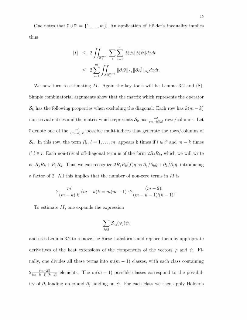
One notes that ı ∪ ıc = 1, . . . ,m. An application of Holder’s inequality implies
thus
|I| ≤ 2
∫∫Rm+1
+
∑ı
m∑i=1
|∂iϕı||∂iψı|dxdt
≤ 2m∑
i=1
∫∫Rm+1
+
‖∂iϕ‖Λk‖∂iψ‖Λk
dxdt.
We now turn to estimating II. Again the key tools will be Lemma 3.2 and (S).
Simple combinatorial arguments show that the matrix which represents the operator
Sk has the following properties when excluding the diagonal: Each row has k(m− k)
non-trivial entries and the matrix which represents Sk has m!(m−k)!k!
rows/columns. Let
ı denote one of the m!(m−k)!k!
possible multi-indices that generate the rows/columns of
Sk. In this row, the term Rl, l = 1, . . . ,m, appears k times if l ∈ ıc and m− k times
if l ∈ ı. Each non-trivial off-diagonal term is of the form 2RjRk, which we will write
as RjRk +RjRk. Thus we can recognize 2RjRk(f)g as ∂j f∂kg + ∂kf∂j g, introducing
a factor of 2. All this implies that the number of non-zero terms in II is
2m!
(m− k)!k!(m− k)k = m(m− 1) · 2 (m− 2)!
(m− k − 1)!(k − 1)!.
To estimate II, one expands the expression
∑ı6=
Sı,(ϕ)ψı
and uses Lemma 3.2 to remove the Riesz transforms and replace them by appropriate
derivatives of the heat extensions of the components of the vectors ϕ and ψ. Fi-
nally, one divides all these terms into m(m − 1) classes, with each class containing
2 (m−2)!(m−k−1)!(k−1)!
elements. The m(m − 1) possible classes correspond to the possibil-
ity of ∂i landing on ϕ and ∂j landing on ψ. For each class we then apply Holder’s
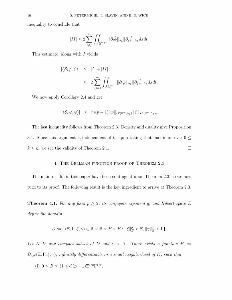
16 S. PETERMICHL, L. SLAVIN, AND B. D. WICK
inequality to conclude that
|II| ≤ 2m∑
i6=j
∫∫Rm+1
+
‖∂iφ‖Λk‖∂jψ‖Λk
dxdt.
This estimate, along with I yields
|〈Skϕ, ψ〉| ≤ |I|+ |II|
≤ 2m∑
i,j=1
∫∫Rm+1
+
‖∂iϕ‖Λk‖∂jψ‖Λk
dxdt.
We now apply Corollary 2.4 and get
|〈Skϕ, ψ〉| ≤ m(p− 1)‖ϕ‖Lp(Rm;Λk)‖ψ‖Lq(Rm;Λk).
The last inequality follows from Theorem 2.3. Density and duality give Proposition
3.1. Since this argument is independent of k, upon taking that maximum over 0 ≤
k ≤ m we see the validity of Theorem 2.1.
4. The Bellman function proof of Theorem 2.3
The main results in this paper have been contingent upon Theorem 2.3, so we now
turn to its proof. The following result is the key ingredient to arrive at Theorem 2.3.
Theorem 4.1. For any fixed p ≥ 2, its conjugate exponent q, and Hilbert space E
define the domain
D := (Ξ,Γ, ξ, γ) ∈ R× R× E × E : ‖ξ‖pE < Ξ, ‖γ‖q
E < Γ.
Let K be any compact subset of D and ε > 0. There exists a function B :=
Bε,K(Ξ,Γ, ξ, γ), infinitely differentiable in a small neighborhood of K, such that
(i) 0 ≤ B ≤ (1 + ε)(p− 1)Ξ1/pΓ1/q,
17
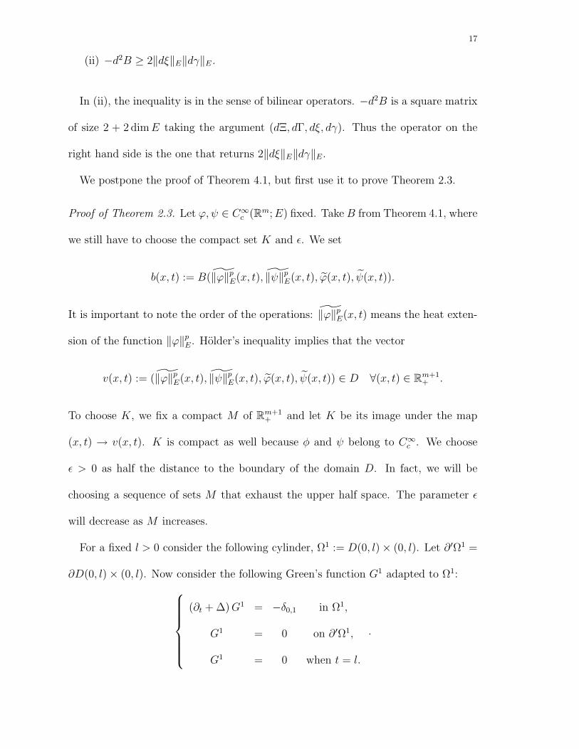
(ii) −d2B ≥ 2‖dξ‖E‖dγ‖E.
In (ii), the inequality is in the sense of bilinear operators. −d2B is a square matrix
of size 2 + 2 dimE taking the argument (dΞ, dΓ, dξ, dγ). Thus the operator on the
right hand side is the one that returns 2‖dξ‖E‖dγ‖E.
We postpone the proof of Theorem 4.1, but first use it to prove Theorem 2.3.
Proof of Theorem 2.3. Let ϕ, ψ ∈ C∞c (Rm;E) fixed. Take B from Theorem 4.1, where
we still have to choose the compact set K and ε. We set
b(x, t) := B(‖ϕ‖pE(x, t), ‖ψ‖p
E(x, t), ϕ(x, t), ψ(x, t)).
It is important to note the order of the operations: ‖ϕ‖pE(x, t) means the heat exten-
sion of the function ‖ϕ‖pE. Holder’s inequality implies that the vector
v(x, t) := (‖ϕ‖pE(x, t), ‖ψ‖p
E(x, t), ϕ(x, t), ψ(x, t)) ∈ D ∀(x, t) ∈ Rm+1+ .
To choose K, we fix a compact M of Rm+1+ and let K be its image under the map
(x, t) → v(x, t). K is compact as well because φ and ψ belong to C∞c . We choose
ε > 0 as half the distance to the boundary of the domain D. In fact, we will be
choosing a sequence of sets M that exhaust the upper half space. The parameter ε
will decrease as M increases.
For a fixed l > 0 consider the following cylinder, Ω1 := D(0, l)× (0, l). Let ∂′Ω1 =
∂D(0, l)× (0, l). Now consider the following Green’s function G1 adapted to Ω1:(∂t + ∆)G1 = −δ0,1 in Ω1,
G1 = 0 on ∂′Ω1,
G1 = 0 when t = l.
.
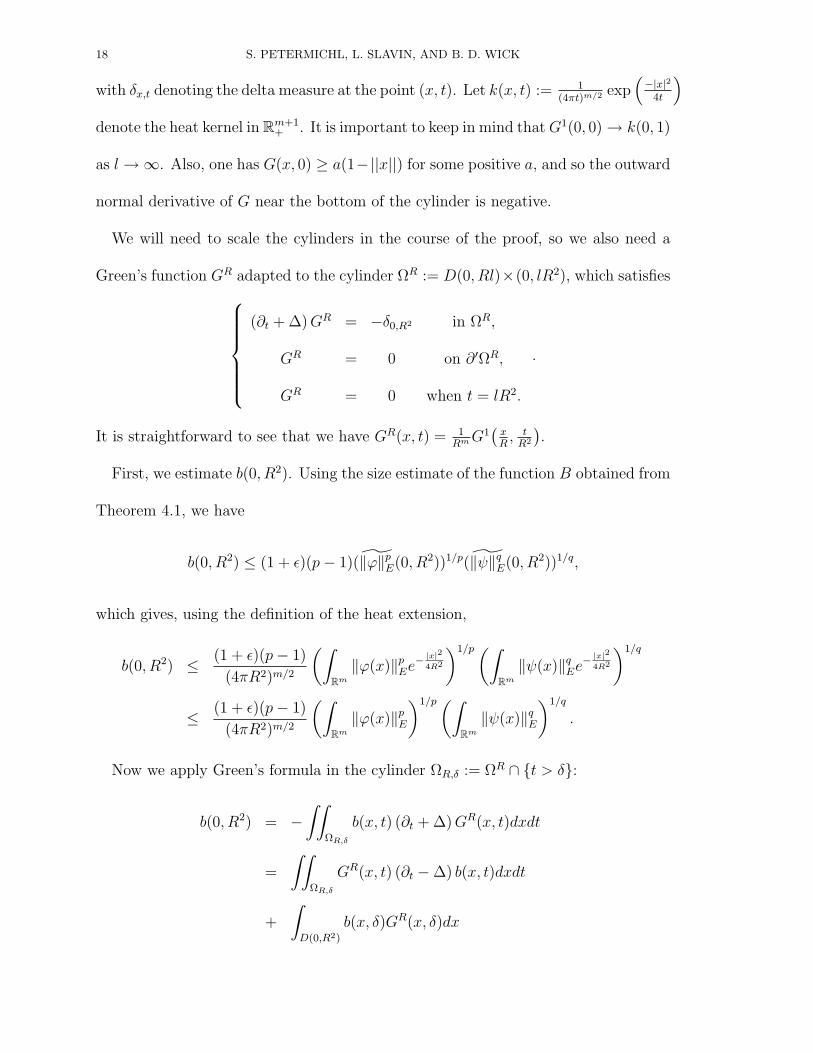
18 S. PETERMICHL, L. SLAVIN, AND B. D. WICK
with δx,t denoting the delta measure at the point (x, t). Let k(x, t) := 1(4πt)m/2 exp
(−|x|2
4t
)denote the heat kernel in Rm+1
+ . It is important to keep in mind thatG1(0, 0) → k(0, 1)
as l→∞. Also, one has G(x, 0) ≥ a(1−||x||) for some positive a, and so the outward
normal derivative of G near the bottom of the cylinder is negative.
We will need to scale the cylinders in the course of the proof, so we also need a
Green’s function GR adapted to the cylinder ΩR := D(0, Rl)×(0, lR2), which satisfies(∂t + ∆)GR = −δ0,R2 in ΩR,
GR = 0 on ∂′ΩR,
GR = 0 when t = lR2.
.
It is straightforward to see that we have GR(x, t) = 1RmG
1(
xR, t
R2
).
First, we estimate b(0, R2). Using the size estimate of the function B obtained from
Theorem 4.1, we have
b(0, R2) ≤ (1 + ε)(p− 1)(‖ϕ‖pE(0, R2))1/p(‖ψ‖q
E(0, R2))1/q,
which gives, using the definition of the heat extension,
b(0, R2) ≤ (1 + ε)(p− 1)
(4πR2)m/2
(∫Rm
‖ϕ(x)‖pEe
− |x|2
4R2
)1/p(∫Rm
‖ψ(x)‖qEe
− |x|2
4R2
)1/q
≤ (1 + ε)(p− 1)
(4πR2)m/2
(∫Rm
‖ϕ(x)‖pE
)1/p(∫Rm
‖ψ(x)‖qE
)1/q
.
Now we apply Green’s formula in the cylinder ΩR,δ := ΩR ∩ t > δ:
b(0, R2) = −∫∫
ΩR,δ
b(x, t) (∂t + ∆)GR(x, t)dxdt
=
∫∫ΩR,δ
GR(x, t) (∂t −∆) b(x, t)dxdt
+
∫D(0,R2)
b(x, δ)GR(x, δ)dx
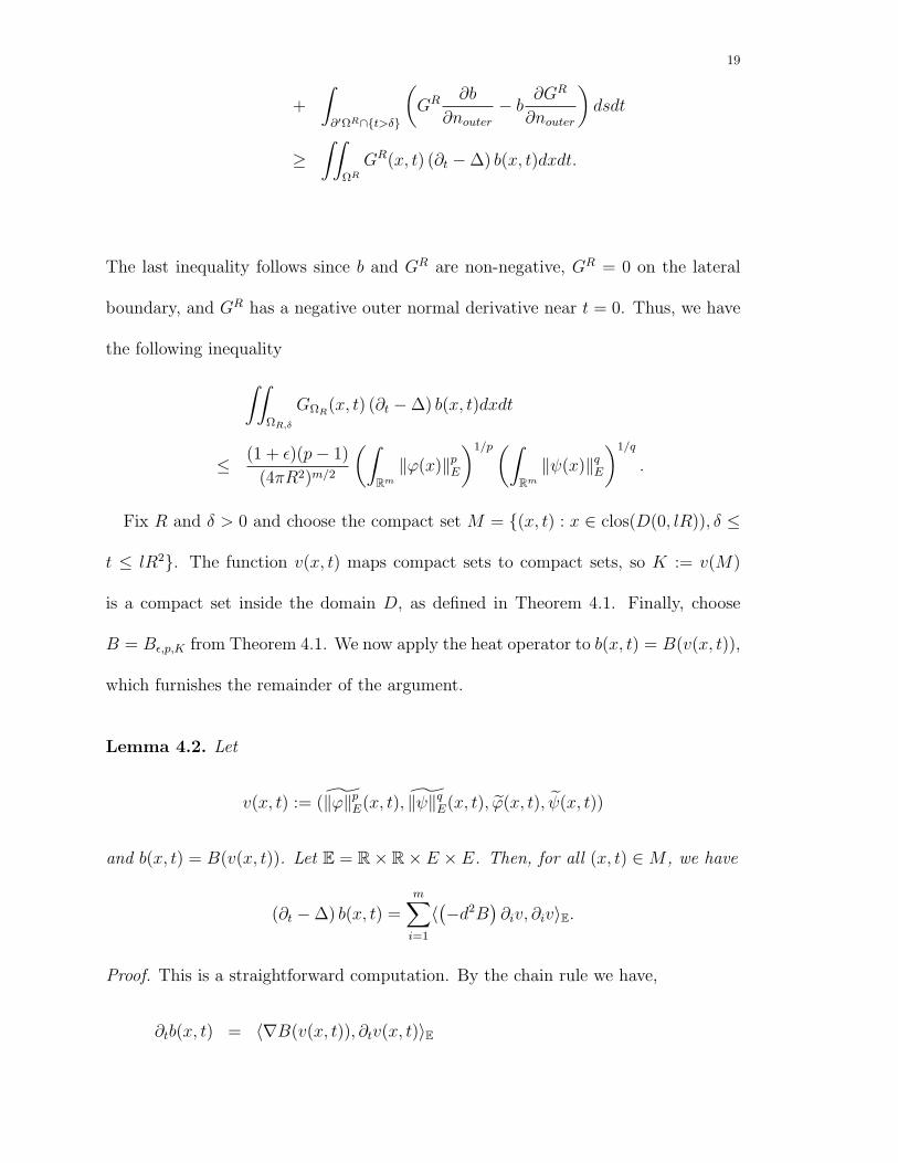
19
+
∫∂′ΩR∩t>δ
(GR ∂b
∂nouter
− b∂GR
∂nouter
)dsdt
≥∫∫
ΩR
GR(x, t) (∂t −∆) b(x, t)dxdt.
The last inequality follows since b and GR are non-negative, GR = 0 on the lateral
boundary, and GR has a negative outer normal derivative near t = 0. Thus, we have
the following inequality∫∫ΩR,δ
GΩR(x, t) (∂t −∆) b(x, t)dxdt
≤ (1 + ε)(p− 1)
(4πR2)m/2
(∫Rm
‖ϕ(x)‖pE
)1/p(∫Rm
‖ψ(x)‖qE
)1/q
.
Fix R and δ > 0 and choose the compact set M = (x, t) : x ∈ clos(D(0, lR)), δ ≤
t ≤ lR2. The function v(x, t) maps compact sets to compact sets, so K := v(M)
is a compact set inside the domain D, as defined in Theorem 4.1. Finally, choose
B = Bε,p,K from Theorem 4.1. We now apply the heat operator to b(x, t) = B(v(x, t)),
which furnishes the remainder of the argument.
Lemma 4.2. Let
v(x, t) := (‖ϕ‖pE(x, t), ‖ψ‖q
E(x, t), ϕ(x, t), ψ(x, t))
and b(x, t) = B(v(x, t)). Let E = R× R× E × E. Then, for all (x, t) ∈M , we have
(∂t −∆) b(x, t) =m∑
i=1
〈(−d2B
)∂iv, ∂iv〉E.
Proof. This is a straightforward computation. By the chain rule we have,
∂tb(x, t) = 〈∇B(v(x, t)), ∂tv(x, t)〉E
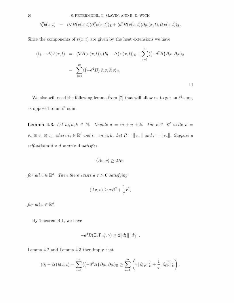
20 S. PETERMICHL, L. SLAVIN, AND B. D. WICK
∂2i b(x, t) = 〈∇B(v(x, t))∂2
i v(x, t)〉E + 〈d2B(v(x, t))∂iv(x, t), ∂iv(x, t)〉E.
Since the components of v(x, t) are given by the heat extensions we have
(∂t −∆) b(x, t) = 〈∇B(v(x, t)), (∂t −∆) v(x, t)〉E +m∑
i=1
〈(−d2B
)∂iv, ∂iv〉E
=m∑
i=1
〈(−d2B
)∂iv, ∂iv〉E.
We also will need the following lemma from [7] that will allow us to get an `2 sum,
as opposed to an `1 sum.
Lemma 4.3. Let m,n, k ∈ N. Denote d = m + n + k. For v ∈ Rd write v =
vm ⊕ vn ⊕ vk, where vi ∈ Ri and i = m,n, k. Let R = ‖vm‖ and r = ‖vn‖. Suppose a
self-adjoint d× d matrix A satisfies
〈Av, v〉 ≥ 2Rr,
for all v ∈ Rd. Then there exists a τ > 0 satisfying
〈Av, v〉 ≥ τR2 +1
τr2,
for all v ∈ Rd.
By Theorem 4.1, we have
−d2B(Ξ,Γ, ξ, γ) ≥ 2‖dξ‖‖dγ‖.
Lemma 4.2 and Lemma 4.3 then imply that
(∂t −∆) b(x, t) =m∑
i=1
〈(−d2B
)∂iv, ∂iv〉E ≥
m∑i=1
(τ‖∂iϕ‖2
E +1
τ‖∂iψ‖2
E
).
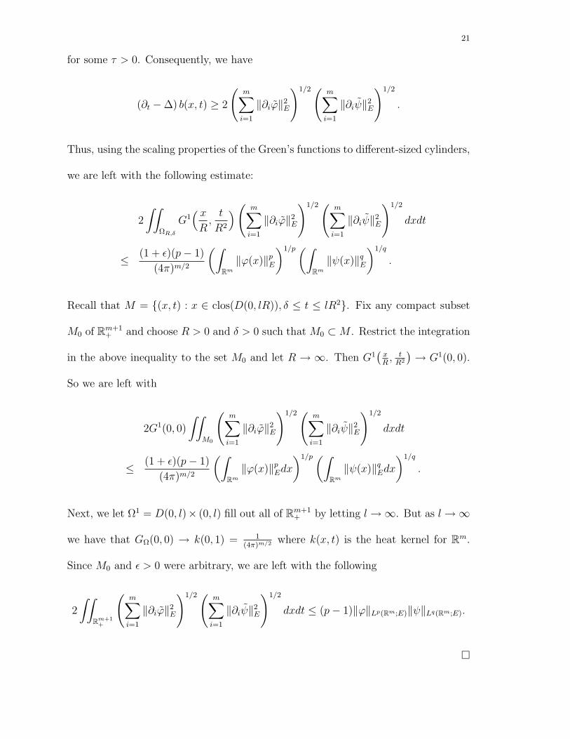
21
for some τ > 0. Consequently, we have
(∂t −∆) b(x, t) ≥ 2
(m∑
i=1
‖∂iϕ‖2E
)1/2( m∑i=1
‖∂iψ‖2E
)1/2
.
Thus, using the scaling properties of the Green’s functions to different-sized cylinders,
we are left with the following estimate:
2
∫∫ΩR,δ
G1( xR,t
R2
)( m∑i=1
‖∂iϕ‖2E
)1/2( m∑i=1
‖∂iψ‖2E
)1/2
dxdt
≤ (1 + ε)(p− 1)
(4π)m/2
(∫Rm
‖ϕ(x)‖pE
)1/p(∫Rm
‖ψ(x)‖qE
)1/q
.
Recall that M = (x, t) : x ∈ clos(D(0, lR)), δ ≤ t ≤ lR2. Fix any compact subset
M0 of Rm+1+ and choose R > 0 and δ > 0 such that M0 ⊂M . Restrict the integration
in the above inequality to the set M0 and let R → ∞. Then G1(
xR, t
R2
)→ G1(0, 0).
So we are left with
2G1(0, 0)
∫∫M0
(m∑
i=1
‖∂iϕ‖2E
)1/2( m∑i=1
‖∂iψ‖2E
)1/2
dxdt
≤ (1 + ε)(p− 1)
(4π)m/2
(∫Rm
‖ϕ(x)‖pEdx
)1/p(∫Rm
‖ψ(x)‖qEdx
)1/q
.
Next, we let Ω1 = D(0, l)× (0, l) fill out all of Rm+1+ by letting l→∞. But as l→∞
we have that GΩ(0, 0) → k(0, 1) = 1(4π)m/2 where k(x, t) is the heat kernel for Rm.
Since M0 and ε > 0 were arbitrary, we are left with the following
2
∫∫Rm+1
+
(m∑
i=1
‖∂iϕ‖2E
)1/2( m∑i=1
‖∂iψ‖2E
)1/2
dxdt ≤ (p− 1)‖ϕ‖Lp(Rm;E)‖ψ‖Lq(Rm;E).
22 S. PETERMICHL, L. SLAVIN, AND B. D. WICK
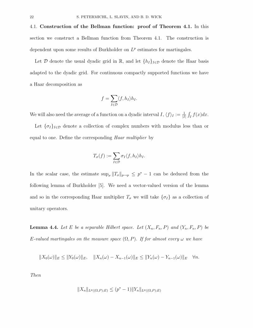
4.1. Construction of the Bellman function: proof of Theorem 4.1. In this
section we construct a Bellman function from Theorem 4.1. The construction is
dependent upon some results of Burkholder on Lp estimates for martingales.
Let D denote the usual dyadic grid in R, and let hII∈D denote the Haar basis
adapted to the dyadic grid. For continuous compactly supported functions we have
a Haar decomposition as
f =∑I∈D
〈f, hI〉hI .
We will also need the average of a function on a dyadic interval I, 〈f〉I := 1|I|
∫If(x)dx.
Let σII∈D denote a collection of complex numbers with modulus less than or
equal to one. Define the corresponding Haar multiplier by
Tσ(f) :=∑I∈D
σI〈f, hI〉hI .
In the scalar case, the estimate supσ ‖Tσ‖p→p ≤ p∗ − 1 can be deduced from the
following lemma of Burkholder [5]. We need a vector-valued version of the lemma
and so in the corresponding Haar multiplier Tσ we will take σI as a collection of
unitary operators.
Lemma 4.4. Let E be a separable Hilbert space. Let (Xn, Fn, P ) and (Yn, Fn, P ) be
E-valued martingales on the measure space (Ω, P ). If for almost every ω we have
‖X0(ω)‖E ≤ ‖Y0(ω)‖E, ‖Xn(ω)−Xn−1(ω)‖E ≤ ‖Yn(ω)− Yn−1(ω)‖E ∀n.
Then
‖Xn‖Lp((Ω,P );E) ≤ (p∗ − 1)‖Yn‖Lp((Ω,P );E)
23
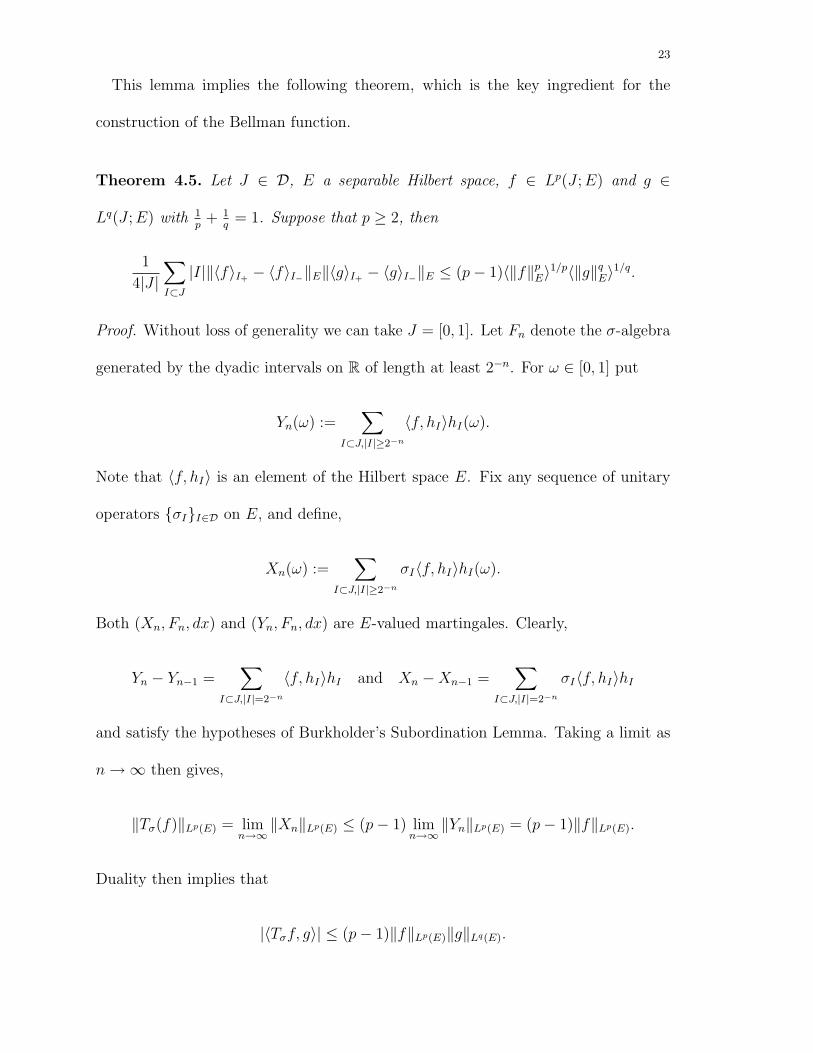
This lemma implies the following theorem, which is the key ingredient for the
construction of the Bellman function.
Theorem 4.5. Let J ∈ D, E a separable Hilbert space, f ∈ Lp(J ;E) and g ∈
Lq(J ;E) with 1p
+ 1q
= 1. Suppose that p ≥ 2, then
1
4|J |∑I⊂J
|I|‖〈f〉I+ − 〈f〉I−‖E‖〈g〉I+ − 〈g〉I−‖E ≤ (p− 1)〈‖f‖pE〉
1/p〈‖g‖qE〉
1/q.
Proof. Without loss of generality we can take J = [0, 1]. Let Fn denote the σ-algebra
generated by the dyadic intervals on R of length at least 2−n. For ω ∈ [0, 1] put
Yn(ω) :=∑
I⊂J,|I|≥2−n
〈f, hI〉hI(ω).
Note that 〈f, hI〉 is an element of the Hilbert space E. Fix any sequence of unitary
operators σII∈D on E, and define,
Xn(ω) :=∑
I⊂J,|I|≥2−n
σI〈f, hI〉hI(ω).
Both (Xn, Fn, dx) and (Yn, Fn, dx) are E-valued martingales. Clearly,
Yn − Yn−1 =∑
I⊂J,|I|=2−n
〈f, hI〉hI and Xn −Xn−1 =∑
I⊂J,|I|=2−n
σI〈f, hI〉hI
and satisfy the hypotheses of Burkholder’s Subordination Lemma. Taking a limit as
n→∞ then gives,
‖Tσ(f)‖Lp(E) = limn→∞
‖Xn‖Lp(E) ≤ (p− 1) limn→∞
‖Yn‖Lp(E) = (p− 1)‖f‖Lp(E).
Duality then implies that
|〈Tσf, g〉| ≤ (p− 1)‖f‖Lp(E)‖g‖Lq(E).
24 S. PETERMICHL, L. SLAVIN, AND B. D. WICK
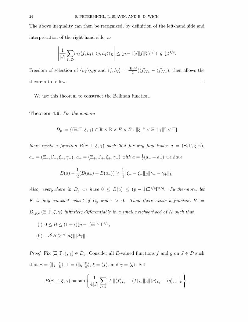
The above inequality can then be recognized, by definition of the left-hand side and
interpretation of the right-hand side, as∣∣∣∣∣ 1
|J |∑I∈D
〈σI〈f, hI〉, 〈g, hI〉〉E
∣∣∣∣∣ ≤ (p− 1)〈‖f‖pE〉
1/p〈‖g‖qE〉
1/q.
Freedom of selection of σII∈D and 〈f, hI〉 = |I|1/2
2(〈f〉I+ − 〈f〉I−), then allows the
theorem to follow.
We use this theorem to construct the Bellman function.
Theorem 4.6. For the domain
Dp := (Ξ,Γ, ξ, γ) ∈ R× R× E × E : ‖ξ‖p < Ξ, ‖γ‖q < Γ
there exists a function B(Ξ,Γ, ξ, γ) such that for any four-tuples a = (Ξ,Γ, ξ, γ),
a− = (Ξ−,Γ−, ξ−, γ−), a+ = (Ξ+,Γ+, ξ+, γ+) with a = 12(a− + a+) we have
B(a)− 1
2(B(a+) +B(a−)) ≥ 1
4‖ξ− − ξ+‖E‖γ− − γ+‖E.
Also, everywhere in Dp we have 0 ≤ B(a) ≤ (p − 1)Ξ1/pΓ1/q. Furthermore, let
K be any compact subset of Dp and ε > 0. Then there exists a function B :=
Bε,p,K(Ξ,Γ, ξ, γ) infinitely differentiable in a small neighborhood of K such that
(i) 0 ≤ B ≤ (1 + ε)(p− 1)Ξ1/pΓ1/q,
(ii) −d2B ≥ 2‖dξ‖‖dγ‖.
Proof. Fix (Ξ,Γ, ξ, γ) ∈ Dp. Consider all E-valued functions f and g on J ∈ D such
that Ξ = 〈‖f‖pE〉, Γ = 〈‖g‖p
E〉, ξ = 〈f〉, and γ = 〈g〉. Set
B(Ξ,Γ, ξ, γ) := sup
1
4|J |∑I⊂J
|I|‖〈f〉I+ − 〈f〉I−‖E‖〈g〉I+ − 〈g〉I−‖E
.
25
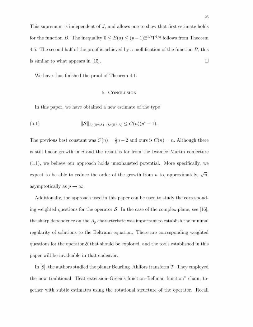
This supremum is independent of J , and allows one to show that first estimate holds
for the function B. The inequality 0 ≤ B(a) ≤ (p− 1)Ξ1/pΓ1/q follows from Theorem
4.5. The second half of the proof is achieved by a mollification of the function B, this
is similar to what appears in [15].
We have thus finished the proof of Theorem 4.1.
5. Conclusion
In this paper, we have obtained a new estimate of the type
(5.1) ‖S‖Lp(Rn;Λ)→Lp(Rn;Λ) ≤ C(n)(p∗ − 1).
The previous best constant was C(n) = 43n− 2 and ours is C(n) = n. Although there
is still linear growth in n and the result is far from the Iwaniec–Martin conjecture
(1.1), we believe our approach holds unexhausted potential. More specifically, we
expect to be able to reduce the order of the growth from n to, approximately,√n,
asymptotically as p→∞.
Additionally, the approach used in this paper can be used to study the correspond-
ing weighted questions for the operator S. In the case of the complex plane, see [16],
the sharp dependence on the Ap characteristic was important to establish the minimal
regularity of solutions to the Beltrami equation. There are corresponding weighted
questions for the operator S that should be explored, and the tools established in this
paper will be invaluable in that endeavor.
In [8], the authors studied the planar Beurling–Ahlfors transform T . They employed
the now traditional “Heat extension–Green’s function–Bellman function” chain, to-
gether with subtle estimates using the rotational structure of the operator. Recall
26 S. PETERMICHL, L. SLAVIN, AND B. D. WICK
that T = R21−R2
2 +2iR1R2 and the part 2R1R2 is just a rotation of the part R21−R2
2.
Estimating the two separately yields the estimate
(5.2) ‖T ‖p→p ≤ 2(p∗ − 1).
We believe that the 2 in (5.2) is the equivalent of our n, since T is just S acting on
1-forms on R2. Volberg and Dragicevic estimated the modified operator
Tθ = (R21 −R2
2) cos θ + 2R1R2 sin θ)
and were able to reduce the 2 in (5.2) to approximately√
2, for large p. One can
then interpolate between these two estimates to produce a significant reduction of
the estimate for all p.
We intend to concentrate on the action of the generalized operator S on forms in
even dimensions, an application particularly important for quasiregular mappings ([12]).
In this setting, it seems very plausible that
‖S‖Lp(R2m;Λ)→Lp(R2m;Λ) = ‖S‖Lp(R2m;Λm)→Lp(R2m;Λm),
due to the block structure of operator S and the obvious symmetry. One then observes
that the “middle” block Sm exhibits a rotation-like structure, very similar to that of
T . It is this structure that we intend to exploit, hoping, therefore, to obtain
C(n) ≈√n
for large p. If that is successful, we can again interpolate obtaining a much improved
estimate for all p.
27
References
[1] Rodrigo Banuelos and Prabhu Janakiraman, Lp-bounds for the Beurling-Ahlfors transform,
Tras. Amer. Math. Soc. (to appear).
[2] Rodrigo Banuelos and Arthur Lindeman II, A martingale study of the Beurling–Ahlfors trans-
form in Rn, J. Funct. Anal. 145 (1997), no. 1, 224–265.
[3] Rodrigo Banuelos and Pedro J. Mendez-Hernandez, Sharp inequalities for heat kernels of
Schrodinger operators and applications to spectral gaps, J. Funct. Anal. 176 (2000), no. 2,
368–399.
[4] Rodrigo Banuelos and Gang Wang, Sharp inequalities for martingales with applications to the
Beurling-Ahlfors and Riesz transforms, Duke Math. J. 80 (1995), no. 3, 575–600.
[5] Donald L. Burkholder, Explorations in martingale theory and its applications, Ecole d’Ete de
Probabilites de Saint-Flour XIX - 1989, Lecture Notes in Math., vol. 1464, Springer. Berlin,
1991, pp. 1–66.
[6] Oliver Dragicevic, Sergei Treil, and Alexander Volberg, A Theorem about Three Quadratic
Forms, preprint at arXiv:0710.3249.
[7] Oliver Dragicevic and Alexander Volberg, Bellman functions and dimensionless estimates of
Littlewood–Paley type, J. Operator Theory 56 (2006), no. 1, 167–198.
[8] , Bellman function, Littlewood-Paley estimates and asymptotics for the Ahlfors-Beurling
operator in Lp(C), Indiana Univ. Math. J. 54 (2005), no. 4, 971–995.
[9] , Bellman function for the estimates of Littlewood-Paley type and asymptotic estimates
in the p− 1 problem, C. R. Math. Acad. Sci. Paris 340 (2005), no. 10, 731–734 (English, with
English and French summaries).
[10] Robert A. Fefferman, Carlos E. Kenig, and Jill C. Pipher, The theory of weights and the Dirichlet
problem for elliptic equations, Ann. of Math. (2) 134 (1991), no. 1, 65–124.
[11] Tadeusz Iwaniec, Extremal inequalities in Sobolev spaces and quasiconformal mappings, Z. Anal.
Anwendungen 1 (1982), no. 6, 1–16.
28 S. PETERMICHL, L. SLAVIN, AND B. D. WICK
[12] Tadeusz Iwaniec and Gaven Martin, Geometric function theory and non-linear analysis, Oxford
Mathematical Monographs, The Clarendon Press Oxford University Press, New York, 2001.
[13] , Riesz transforms and related singular integrals, J. Reine Angew. Math. 473 (1996),
25–57.
[14] , Quasiregular mappings in even dimensions, Acta Math. 170 (1993), no. 1, 29–81.
[15] Fedor Nazarov and Alexander Volberg, Heat extension of the Beurling operator and estimates
for its norm, Algebra i Analiz 15 (2003), no. 4, 142–158 (Russian, with Russian summary);
English transl., St. Petersburg Math. J. 15 (2004), no. 4, 563–573.
[16] Stefanie Petermichl and Alexander Volberg, Heating of the Ahlfors-Beurling operator: weakly
quasiregular maps on the plane are quasiregular, Duke Math. J. 112 (2002), no. 2, 281–305.
Stefanie Petermichl, Departement de Mathematiques, Universite de Bordeaux 1,
351, Cours de la Liberation, 33405 Talence, France
E-mail address: [email protected]
Leonid Slavin, Department of Mathematics, University of Missouri, Columbia,
Columbia, MO USA 65211
E-mail address: [email protected]
Brett D. Wick, Department of Mathematics, University of South Carolina, Columbia,
SC USA 29208
E-mail address: [email protected]