New aspects of the Yang-Baxter equation
68
New aspects of the Yang-Baxter equation Victoria LEBED Jean Leray Mathematics Institute, University of Nantes Symposium on Mathematical Physics November 10, 2014 ←→
Transcript of New aspects of the Yang-Baxter equation
New aspects of the Yang-Baxter equation
Victoria LEBED
Jean Leray Mathematics Institute, University of Nantes
Symposium on Mathematical Physics
November 10, 2014
←→
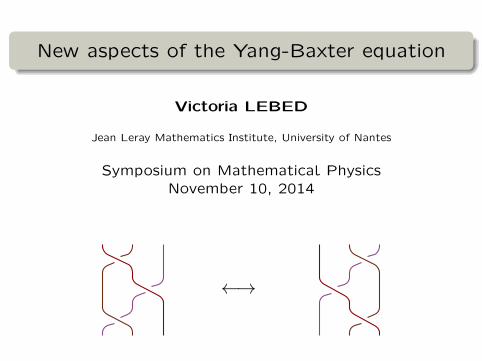
1 Yang-Baxter equation
✓ A vector space V (or an object in any
monoidal category)
✓ σ : V⊗2→ V⊗2
Yang-Baxter equation (YBE):
σ1 ◦σ2 ◦σ1 = σ2 ◦σ1 ◦σ2 : V⊗3→V⊗3
where σi = Id⊗i−1V ⊗σ⊗ Id⊗···
V .
A map σ satisfying YBE is a braiding.
σ ←→
V⊗V
V⊗V
=
(Reidemeister III)

1 Yang-Baxter equation
✓ A vector space V (or an object in any
monoidal category)
✓ σ : V⊗2→ V⊗2
Yang-Baxter equation (YBE):
σ1 ◦σ2 ◦σ1 = σ2 ◦σ1 ◦σ2 : V⊗3→V⊗3
where σi = Id⊗i−1V ⊗σ⊗ Id⊗···
V .
A map σ satisfying YBE is a braiding.
(V,σ) ;
σ ←→
V⊗V
V⊗V
=
(Reidemeister III)
rep. of B+n (pos.
braid monoid):
i i+1 n
7→ σi
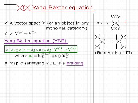
1 Yang-Baxter equation
✓ A vector space V (or an object in any
monoidal category)
✓ σ : V⊗2→ V⊗2
Yang-Baxter equation (YBE):
σ1 ◦σ2 ◦σ1 = σ2 ◦σ1 ◦σ2 : V⊗3→V⊗3
where σi = Id⊗i−1V ⊗σ⊗ Id⊗···
V .
A map σ satisfying YBE is a braiding.
(V,σ) ;
σ is invertible ;
σ ←→
V⊗V
V⊗V
=
(Reidemeister III)
rep. of B+n (pos.
braid monoid):
i i+1 n
7→ σi
rep. of Bn (braid
group)
7→ σ−1i

2 YBE in physics
✓ Particle physics: factorization condition for the dispersion
matrix in the 1-dim. n-body problem (McGuire, Yang, 60’).
collisions ←→

2 YBE in physics
✓ Particle physics: factorization condition for the dispersion
matrix in the 1-dim. n-body problem (McGuire, Yang, 60’).
collisions ←→
✓ Statistical mechanics: partition function for exactly
solvable lattice models (Onsager, 1944, Ising model;
Baxter, 70’, 8-vertex, hard hexagon & chiral Potts models).
Boltzmann
weights

2 YBE in physics
✓ Particle physics: factorization condition for the dispersion
matrix in the 1-dim. n-body problem (McGuire, Yang, 60’).
collisions ←→
✓ Statistical mechanics: partition function for exactly
solvable lattice models (Onsager, 1944, Ising model;
Baxter, 70’, 8-vertex, hard hexagon & chiral Potts models).
✓ Quantum inverse scattering method for completely
integrable systems (Faddeev et al., 1979).
✓ Factorizable S-matrices in 2-dim. quantum field theory
(Zamolodchikov, 1979).
✓ Quantum group (Drinfel ′d, 80’).
✓ C∗ algebras (Woronowicz, 80’).
✓ Conformal field theory.

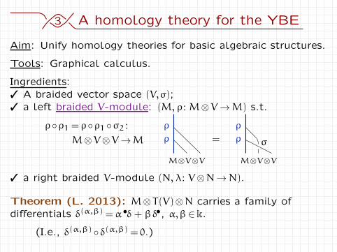
3 A homology theory for the YBE
Aim: Unify homology theories for basic algebraic structures.

3 A homology theory for the YBE
Aim: Unify homology theories for basic algebraic structures.
Tools: Graphical calculus.

3 A homology theory for the YBE
Aim: Unify homology theories for basic algebraic structures.
Tools: Graphical calculus.
Ingredients:
✓ A braided vector space (V,σ);
✓ a left braided V-module: (M, ρ : M⊗V→M) s.t.
ρ◦ρ1 = ρ◦ρ1 ◦σ2 :
M⊗V⊗V→M
ρ
ρ
M⊗V⊗V
=
ρ
ρ
M⊗V⊗V
σ
✓ a right braided V-module (N, λ : V⊗N→N).
Theorem (L. 2013): M⊗T(V)⊗N carries a family of
differentials δ(α,β) = α•δ + βδ•, α,β∈ k.
(I.e., δ(α,β) ◦δ(α,β) = 0.)

3 A homology theory for the YBE
Theorem (L. 2013): M⊗T(V)⊗N carries a family of
differentials δ(α,β) = α•δ + βδ•, α,β∈ k.
•δ=∑
(−1)i−1
ρσ
σ
1 ... i ...n
V ... VM N
δ• =∑
(−1)i−1
λ
σ
σ
1 ... i ... n
V ... VM N

3 A homology theory for the YBE
Theorem (L. 2013): M⊗T(V)⊗N carries a family of
differentials δ(α,β) = α•δ + βδ•, α,β∈ k.
•δ=∑
(−1)i−1
ρσ
σ
1 ... i ...n
V ... VM N
δ• =∑
(−1)i−1
λ
σ
σ
1 ... i ... n
V ... VM N
Proof:
YBE=
br. mod.=
& sign =
(−1)#cross.

3 A homology theory for the YBE
Theorem (L. 2013): M⊗T(V)⊗N carries a family of
differentials δ(α,β) = α•δ + βδ•, α,β∈ k.
•δ=∑
(−1)i
ρσ
σ
1 ... i ...n
V ... VM N
δ• =∑
(−1)i
λ
σ
σ
1 ... i ... n
V... VM N
Remarks:
✓ Functoriality.
✓ Interpretation in terms of quantum shuffles (Rosso, 1995).
✓ Duality ; a cohomology theory.
✓ Pre-cubical structure.

3 A homology theory for the YBE
Theorem (L. 2013): M⊗T(V)⊗N carries a family of
differentials δ(α,β) = α•δ + βδ•, α,β∈ k.
Remarks:
✓ Functoriality.
✓ Interpretation in terms of quantum shuffles (Rosso, 1995).
✓ Duality ; a cohomology theory.
✓ Pre-cubical structure.
✓ Degeneracies.
Braided coalgebra: br. v. sp. (V,σ) & ∆ : V→ V⊗V s.t.
= = =
B Cf. Reidemeister moves for knotted 3-valent graphs!
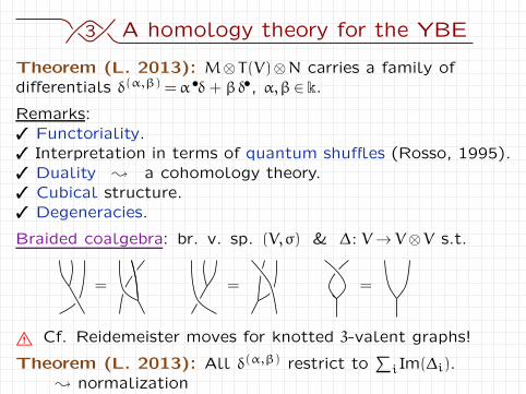
3 A homology theory for the YBE
Theorem (L. 2013): M⊗T(V)⊗N carries a family of
differentials δ(α,β) = α•δ + βδ•, α,β∈ k.
Remarks:
✓ Functoriality.
✓ Interpretation in terms of quantum shuffles (Rosso, 1995).
✓ Duality ; a cohomology theory.
✓ Cubical structure.
✓ Degeneracies.
Braided coalgebra: br. v. sp. (V,σ) & ∆ : V→ V⊗V s.t.
= = =
B Cf. Reidemeister moves for knotted 3-valent graphs!
Theorem (L. 2013): All δ(α,β) restrict to∑
i Im(∆i).
; normalization
4 Alg. structures via braidings
A Associative algebras

4 Alg. structures via braidings
A Associative algebras
(V, µ : V⊗V→ V, ξ : k→V), ξ(α) =α1V , s.t.
Associativity:µ◦µ1 = µ◦µ2
=
Unit axiom:µ◦ξ1 = µ◦ξ2 = IdV
= =

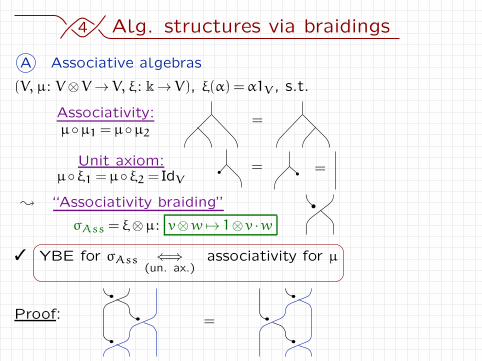
4 Alg. structures via braidings
A Associative algebras
(V, µ : V⊗V→ V, ξ : k→V), ξ(α) =α1V , s.t.
Associativity:µ◦µ1 = µ◦µ2
=
Unit axiom:µ◦ξ1 = µ◦ξ2 = IdV
= =
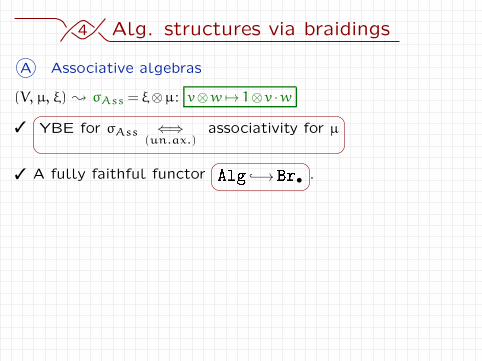
; “Associativity braiding”
σAss = ξ⊗µ : v⊗w 7→ 1⊗v ·w
✓ YBE for σAss ⇐⇒(un. ax.)
associativity for µ
4 Alg. structures via braidings
A Associative algebras
(V, µ : V⊗V→ V, ξ : k→V), ξ(α) =α1V , s.t.
Associativity:µ◦µ1 = µ◦µ2
=
Unit axiom:µ◦ξ1 = µ◦ξ2 = IdV
= =
; “Associativity braiding”
σAss = ξ⊗µ : v⊗w 7→ 1⊗v ·w
✓ YBE for σAss ⇐⇒(un. ax.)
associativity for µ
Proof: =
4 Alg. structures via braidings
A Associative algebras
(V, µ, ξ) ; σAss = ξ⊗µ : v⊗w 7→ 1⊗v ·w
✓ YBE for σAss ⇐⇒(un.ax.)
associativity for µ
✓ A fully faithful functorAlg −֒→ Br•
.

4 Alg. structures via braidings
A Associative algebras
(V, µ, ξ) ; σAss = ξ⊗µ : v⊗w 7→ 1⊗v ·w
✓ YBE for σAss ⇐⇒(un.ax.)
associativity for µ
✓ A fully faithful functorAlg −֒→ Br•
.
✓ Duality: Alg −֒→ Br
•
•←−֓ oAlg.
4 Alg. structures via braidings
A Associative algebras
(V, µ, ξ) ; σAss = ξ⊗µ : v⊗w 7→ 1⊗v ·w
✓ YBE for σAss ⇐⇒(un.ax.)
associativity for µ
✓ A fully faithful functorAlg −֒→ Br•
.
✓ Duality: Alg −֒→ Br
•
•←−֓ oAlg.
✓ σAss ◦σAss = σAss =⇒ highly non-invertible.
✓ Braided modules for (V, σAss) ←→ modules for (V, µ, ξ).
✓ ∆Ass = ξ1 : v 7→ 1⊗v ; braided coalgebra.
✓ Braided homologies for (V, σAss) include
➺ bar differential; ➺ Hochschild; ➺ group hom.

4 Alg. structures via braidings
B Leibniz algebras
(V, µ : V⊗V→ V, ξ : k→V), ξ(α) =α1V , s.t.
Leibniz identity: µ◦µ2 = µ◦µ1−µ◦µ1 ◦τ, where τ : w⊗u→u⊗w
[v, [w,u]] = [[v,w],u]− [[v,u],w]
Lie unit axiom: µ◦ξ2 = µ◦ξ1 = 0
[1,v] = [v,1] = 0
(Bloh 1965, Loday & Cuvier 1991: a non-commutative
generalization of Lie algebras.)
; “Leibniz braiding” σLei = τ+ξ⊗µ : v⊗w 7→w⊗v+1⊗ [v,w]
✓ YBE for σLei ⇐⇒(Lie un. ax.)
Leibniz identity for µ
✓ A fully faithful functorLei −֒→ Br•
.
✓ σLei is invertible.
✓ Braided mod. for (V, σLei) ←→ Leibniz mod. for (V, µ, ξ).
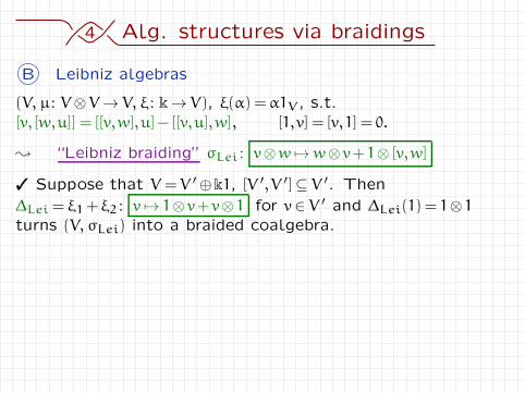
4 Alg. structures via braidings
B Leibniz algebras
(V, µ : V⊗V→ V, ξ : k→V), ξ(α) =α1V , s.t.
[v, [w,u]] = [[v,w],u]− [[v,u],w], [1,v] = [v,1] = 0.
; “Leibniz braiding” σLei : v⊗w 7→w⊗v+1⊗ [v,w]
✓ Suppose that V =V ′⊕k1, [V ′,V ′]⊆ V ′. Then
∆Lei = ξ1+ξ2 : v 7→ 1⊗v+v⊗1 for v∈ V ′ and ∆Lei(1) = 1⊗1
turns (V, σLei) into a braided coalgebra.
✓ Braided homologies for (V, σLei) include Leibniz homology.
(M⊗T(V),dLei)
anti-
symm.����
Cuvier-Loday
Lie
V� // (M⊗Λ(V),dCE) Chevalley-Eilenberg

4 Alg. structures via braidings
B Leibniz algebras
(V, µ : V⊗V→ V, ξ : k→V), ξ(α) =α1V , s.t.
[v, [w,u]] = [[v,w],u]− [[v,u],w], [1,v] = [v,1] = 0.
; “Leibniz braiding” σLei : v⊗w 7→w⊗v+1⊗ [v,w]
✓ Suppose that V =V ′⊕k1, [V ′,V ′]⊆ V ′. Then
∆Lei = ξ1+ξ2 : v 7→ 1⊗v+v⊗1 for v∈ V ′ and ∆Lei(1) = 1⊗1
turns (V, σLei) into a braided coalgebra.
✓ Braided homologies for (V, σLei) include Leibniz homology.
Lei
anti-
symm.����
V� // (M⊗T(V),dLei)
anti-
symm.����
Cuvier-Loday
Lie
?�
OO
V_
OO
� // (M⊗Λ(V),dCE) Chevalley-Eilenberg
✓ Explains the choice of the lift of the Jacobi identity.

4 Alg. structures via braidings
C Self-distributive structures

4 Alg. structures via braidings
C Self-distributive structures
b a�b
a b
colorings
by (S,�)
“SD braiding”
σSD : (a,b) 7→ (b,a�b) ab
c
cb� c (a�b)�c
a�b
RIII←→
ab
c
cb� c (a�c)�(b�c)
a�c
YBE ←→ RIII ←→ (a�b)� c= (a� c)� (b� c) (SD)

4 Alg. structures via braidings
C Self-distributive structures
b a�b
a b
colorings
by (S,�)
“SD braiding”
σSD : (a,b) 7→ (b,a�b) ab
c
cb� c (a�b)�c
a�b
RIII←→
ab
c
cb� c (a�c)�(b�c)
a�c
YBE ←→ RIII ←→ (a�b)� c= (a� c)� (b� c) (SD)

4 Alg. structures via braidings
C Self-distributive structures
b a�b
a b
colorings
by (S,�)
“SD braiding”
σSD : (a,b) 7→ (b,a�b) ab
c
cb� c (a�b)�c
a�b
RIII←→
ab
c
cb� c (a�c)�(b�c)
a�c
YBE ←→ RIII ←→ (a�b)� c= (a� c)� (b� c) (SD)
∃σ−1SD ←→ RII ←→ a 7→ a�b is bijective (Inv)
←→ RI ←→ a�a= a (Idem)
RII←→
RI←→
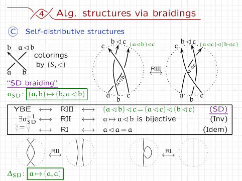
4 Alg. structures via braidings
C Self-distributive structures
b a�b
a b
colorings
by (S,�)
“SD braiding”
σSD : (a,b) 7→ (b,a�b) ab
c
cb� c (a�b)�c
a�b
RIII←→
ab
c
cb� c (a�c)�(b�c)
a�c
YBE ←→ RIII ←→ (a�b)� c= (a� c)� (b� c) (SD)
∃σ−1SD ←→ RII ←→ a 7→ a�b is bijective (Inv)
= ←→ RI ←→ a�a= a (Idem)
RII←→
RI←→
∆SD : a 7→ (a,a)
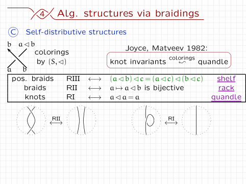
4 Alg. structures via braidings
C Self-distributive structures
b a�b
a b
colorings
by (S,�)
Joyce, Matveev 1982:
knot invariantscolorings
; quandle
pos. braids RIII ←→ (a�b)� c= (a� c)� (b� c) shelf
braids RII ←→ a 7→ a�b is bijective rack
knots RI ←→ a�a= a quandle
RII←→
RI←→
4 Alg. structures via braidings
C Self-distributive structures
b a�b
a b
colorings
by (S,�)
Joyce, Matveev 1982:
knot invariantscolorings
; quandle
pos. braids RIII ←→ (a�b)� c= (a� c)� (b� c) shelf
braids RII ←→ a 7→ a�b is bijective rack
knots RI ←→ a�a= a quandle
Ex.: ➺ Conjugation quandles: (group G, g�h= h−1gh)
coloring rule ←→Wirtinger presentation rule,
colorings ←→ Rep(π1(R3\K),G).
Ex.: ➺ Dihedral quandles: (Zn, a�b= 2b−a)
colorings ←→ n-Fox colorings.
n= 36=
4 Alg. structures via braidings
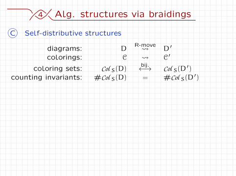
C Self-distributive structures
diagrams: DR-move D ′
colorings: C C ′
coloring sets: Col S(D)bij.←→ Col S(D
′)
counting invariants: #Col S(D) = #Col S(D′)
4 Alg. structures via braidings
C Self-distributive structures
diagrams: DR-move D ′
colorings: C C ′
coloring sets: Col S(D)bij.←→ Col S(D
′)
counting invariants: #Col S(D) = #Col S(D′)
Question: Extract more information?
Idea: Some “weight” ω s.t. ω(C) =ω(C ′)
=⇒ {ω(C) |C ∈ Col S(D) }= {ω(C ′) |C ′ ∈ Col S(D′) }.
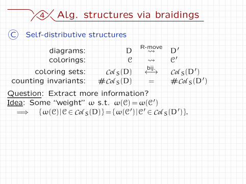
Answer: quandle cocycle invariants (Carter-Jelsovsky-
Kamada-Langford-Saito 1999).
φ : S×S→A ;
Boltzmann weight:ωφ(C) =
∑
a
b
±φ(a,b)

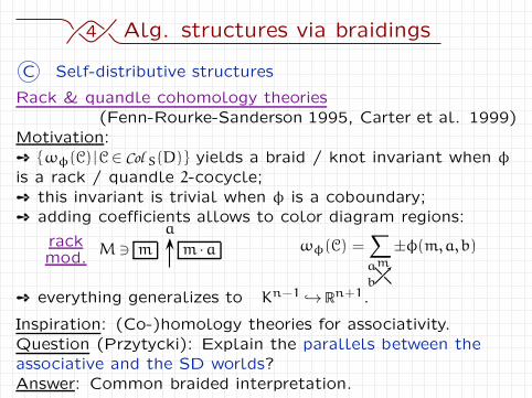
4 Alg. structures via braidings
C Self-distributive structures
Rack & quandle cohomology theories
(Fenn-Rourke-Sanderson 1995, Carter et al. 1999)
Motivation:
➺ {ωφ(C) | C∈ Col S(D) } yields a braid / knot invariant when φ
is a rack / quandle 2-cocycle;
➺ this invariant is trivial when φ is a coboundary;
➺ adding coefficients allows to color diagram regions:a
rackmod.
M∋ m m ·a ωφ(C) =∑
a
b
m
±φ(m,a,b)
➺ everything generalizes to Kn−1 →֒ Rn+1.
Inspiration: (Co-)homology theories for associativity.
Question (Przytycki): Explain the parallels between the
associative and the SD worlds?
Answer: Common braided interpretation.

4 Alg. structures via braidings
C Self-distributive structures
Shelf (S, �) ; σSD : (a,b) 7→ (b,a�b)
✓ YBE for σSD ⇐⇒ SD for �
✓ A fully faithful functorShelf −֒→Br
.
✓ σSD is invertible ⇐⇒ (S, �) is a rack.
✓ Braided modules for (V, σSD) ←→ rack modules for (S, �).
✓ ∆SD : a 7→ (a,a) ; weak braided coalgebra if (S, �) is a
quandle.
✓ Braided homologies for (V, σSD) include rack, quandle,
and other SD homologies.
5 Multi-component braidings
Question: How to treat more complicated structures?

5 Multi-component braidings
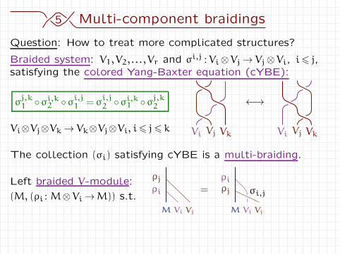
Question: How to treat more complicated structures?
Braided system: V1,V2, . . . ,Vr and σi,j : Vi⊗Vj→ Vj⊗Vi, i6 j,
satisfying the colored Yang-Baxter equation (cYBE):
σj,k1 ◦σ
i,k2 ◦σi,j
1 = σi,j2 ◦σ
i,k1 ◦σ
j,k2
Vi⊗Vj⊗Vk→ Vk⊗Vj⊗Vi, i6 j6 k Vi Vj Vk
←→
Vi Vj Vk
The collection (σi) satisfying cYBE is a multi-braiding.
5 Multi-component braidings
Question: How to treat more complicated structures?
Braided system: V1,V2, . . . ,Vr and σi,j : Vi⊗Vj→ Vj⊗Vi, i6 j,
satisfying the colored Yang-Baxter equation (cYBE):
σj,k1 ◦σ
i,k2 ◦σi,j
1 = σi,j2 ◦σ
i,k1 ◦σ
j,k2
Vi⊗Vj⊗Vk→ Vk⊗Vj⊗Vi, i6 j6 k Vi Vj Vk
←→
Vi Vj Vk
The collection (σi) satisfying cYBE is a multi-braiding.
Left braided V-module:
(M, (ρi : M⊗Vi→M)) s.t.
ρjρi
M Vi Vj
= ρj
ρiσi,j
M Vi Vj
Theorem (L., 2013): M⊗T(V1)⊗·· ·⊗T(Vr)⊗N carries a
family of differentials δ(α,β) =α•δ + βδ•, α,β∈ k.

5 Multi-component braidings
Finite-dim. bialgebra H ;
(H,H∗; σH,H = σrAss(H),σH∗,H∗ = σAss(H
∗),σH,H∗ = σYD)
σH,H = σH∗,H∗ = σH,H∗ =ev
h⊗ l 7→ 〈l(1),h(2)〉l(2)⊗h(1)
✓ YBE on H⊗H∗⊗H∗ ⇐⇒(un. ax.)
bialgebra compatibility

5 Multi-component braidings
Finite-dim. bialgebra H ;
(H,H∗; σH,H = σrAss(H),σH∗,H∗ = σAss(H
∗),σH,H∗ = σYD)
σH,H = σH∗,H∗ = σH,H∗ =ev
h⊗ l 7→ 〈l(1),h(2)〉l(2)⊗h(1)
✓ YBE on H⊗H∗⊗H∗ ⇐⇒(un. ax.)
bialgebra compatibility
✓ A fully faithful functor ∗Bialg −֒→ ∗
2BrSyst•
•.

5 Multi-component braidings
Finite-dim. bialgebra H ;
(H,H∗; σH,H = σrAss(H),σH∗,H∗ = σAss(H
∗),σH,H∗ = σYD)
σH,H = σH∗,H∗ = σH,H∗ =ev
h⊗ l 7→ 〈l(1),h(2)〉l(2)⊗h(1)
✓ YBE on H⊗H∗⊗H∗ ⇐⇒(un. ax.)
bialgebra compatibility
✓ A fully faithful functor ∗Bialg −֒→ ∗
2BrSyst•
•.
✓ σH,H∗ is invertible ⇐⇒ H is a Hopf algebra .
✓ Braided modules ←→ Hopf modules over H.
✓ Braided homologies include
➺ Gerstenhaber-Schack; ➺ Panaite-Ştefan.

5 Multi-component braidings
Finite-dim. bialgebra H ; (H,Hop,H∗,(H∗)op; . . .).
✓ A fully faithful functor ∗Bialg −֒→ ∗
4BrSyst•
•.

5 Multi-component braidings
Finite-dim. bialgebra H ; (H,Hop,H∗,(H∗)op; . . .).
✓ A fully faithful functor ∗Bialg −֒→ ∗
4BrSyst•
•.
✓ Braided modules ←→ Hopf bimodules over H.

5 Multi-component braidings
Finite-dim. bialgebra H ; (H,Hop,H∗,(H∗)op; . . .).
✓ A fully faithful functor ∗Bialg −֒→ ∗
4BrSyst•
•.
✓ Braided modules ←→ Hopf bimodules over H.
Application:
➺ Hopf bimodules are modules over the Heisenberg double
H (H) =H⊗H∗
➺ Cibils-Rosso 1998: “Hopf bimodules are modules” over
X (H) = (H⊗Hop)⊗(H∗⊗ (H∗)op)
➺ Panaite 2002: “Hopf bimodules are modules over ...”
Y (H) =H∗#(Hop⊗H)#(H∗)op &
Z (H) = (H∗⊗ (H∗)op) ⊲⊳ (Hop⊗H)
➺ Theorem (L. 2013): Hopf bimodules are modules over
4!= 24 pairwise isomorphic algebras.
✓ Braided homologies include the Ospel-Taillefer theory.
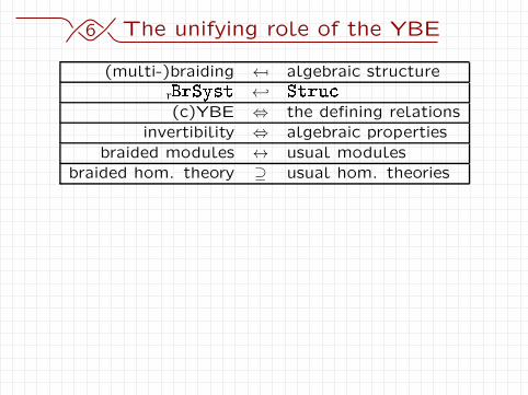
6 The unifying role of the YBE
(multi-)braiding 7→algebraic structure
rBrSyst ←֓ Stru
(c)YBE ⇔ the defining relations
invertibility ⇔ algebraic properties
braided modules ↔ usual modules
braided hom. theory ⊇ usual hom. theories

6 The unifying role of the YBE
(multi-)braiding 7→algebraic structure
rBrSyst ←֓ Stru
(c)YBE ⇔ the defining relations
invertibility ⇔ algebraic properties
braided modules ↔ usual modules
braided hom. theory ⊇ usual hom. theories
Other “braidable” structures:
➺ module algebras (Yau);
➺ Yetter-Drinfel ′d modules (Panaite-Ştefan);
➺ (non-commutative) Poisson algebras (Fresse);
➺ multiple conjugation quandles (Ishii)
knotted
handle-bodies←→