Circuits II - Circuits with Capacitors & Heat Equation

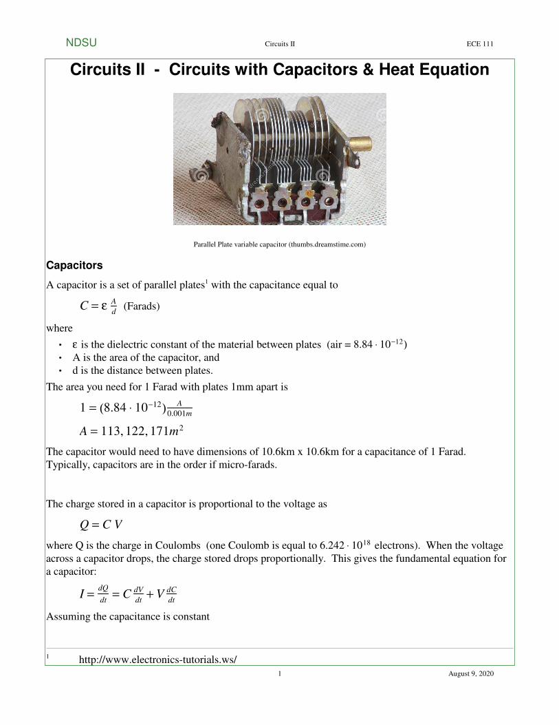
Parallel Plate variable capacitor (thumbs.dreamstime.com)

Capacitors

A capacitor is a set of parallel plates1 with the capacitance equal to

(Farads)C = ε A

d

where

is the dielectric constant of the material between plates (air = ε 8.84 ⋅ 10−12)

A is the area of the capacitor, and

d is the distance between plates.

The area you need for 1 Farad with plates 1mm apart is

1 = (8.84 ⋅ 10−12)A

0.001m

A = 113, 122, 171m2

The capacitor would need to have dimensions of 10.6km x 10.6km for a capacitance of 1 Farad.

Typically, capacitors are in the order if micro-farads.

The charge stored in a capacitor is proportional to the voltage as

Q = C V

where Q is the charge in Coulombs (one Coulomb is equal to electrons). When the voltage6.242 ⋅ 1018

across a capacitor drops, the charge stored drops proportionally. This gives the fundamental equation for

a capacitor:

I =dQ

dt= C

dV

dt+ V

dC

dt

Assuming the capacitance is constant

1 http://www.electronics-tutorials.ws/

NDSU Circuits II ECE 111

1 August 9, 2020

I = CdV

dt

This means that capacitors are integrators:

V = 1

C ∫ I ⋅ dt

In Calculus, you will be covering integration and differentiation and how to come up with a closed-form

solution to various problems. With MATLAB (i.e. in this class) you can solve using numerical methods.

Time Response of an RC filter: (Heat Equation)

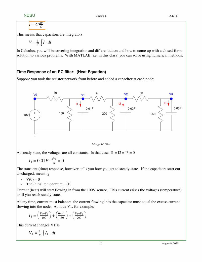
Suppose you took the resistor network from before and added a capacitor at each node:

+

-10V

30 40 50

150 200 250

0.01F 0.02F 0.03F

V0 V1 V2 V3

I1 I2 I3

3-Stage RC Filter

At steady-state, the voltages are all constants. In that case, I1 = I2 = I3 = 0

I1 = 0.01F ⋅dV1

dt= 0

The transient (time) response, however, tells you how you get to steady-state. If the capacitors start out

discharged, meaning

V(0) = 0

The initial temperature = 0C

Current (heat) will start flowing in from the 100V source. This current raises the voltages (temperature)

until you reach steady-state.

At any time, current must balance: the current flowing into the capacitor must equal the excess current

flowing into the node. At node V1, for example:

I1 =

V0−V1

100 +

0−V1

150 +

V2−V1

200

This current changes V1 as

V1 = 1

C ∫ I1 ⋅ dt

NDSU Circuits II ECE 111

2 August 9, 2020

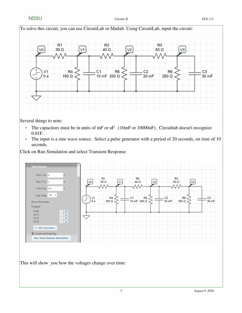
To solve this circuit, you can use CircuitLab or Matlab. Using CircuitLab, input the circuit:

Several things to note:

The capacitors must be in units of mF or uF (10mF or 10000uF). Circuitlab doesn't recognize

0.01F.

The input is a sine wave source. Select a pulse generator with a period of 20 seconds, on time of 10

seconds.

Click on Run Simulation and select Transient Response

This will show you how the voltages change over time:

NDSU Circuits II ECE 111

3 August 9, 2020

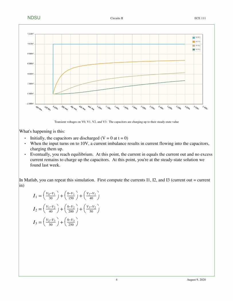
Transient voltages on V0, V1, V2, and V3: The capacitors are charging up to their steady-state value

What's happening is this:

Initially, the capacitors are discharged (V = 0 at t = 0)

When the input turns on to 10V, a current imbalance results in current flowing into the capacitors,

charging them up.

Eventually, you reach equilibrium. At this point, the current in equals the current out and no excess

current remains to charge up the capacitors. At this point, you're at the steady-state solution we

found last week.

In Matlab, you can repeat this simulation. First compute the currents I1, I2, and I3 (current out = current

in)

I1 =

V0−V1

30 +

0−V1

150 +

V2−V1

40

I2 =

V1−V2

40 +

0−V2

200 +

V3−V2

50

I3 =

V2−V3

50 +

0−V3

250

NDSU Circuits II ECE 111

4 August 9, 2020

Note that the current is equal to C dV

dt

0.01dV1

dt= I1 =

V0−V1

30 +

0−V1

150 +

V2−V1

40

0.02dV2

dt= I2 =

V1−V2

40 +

0−V2

200 +

V3−V2

50

0.03dV3

dt= I3 =

V2−V3

50 +

0−V3

250

Solve for dV i

dt

dV1

dt= 3.333V0 − 6.500V1 + 2.500V2

dV2

dt= 1.250V1 − 2.500V2 + 1.000V3

dV3

dt= 0.667V2 − 0.800V3

Integrate to find V1..V3

V1(t) = ∫0

t dV1

dt⋅ dτ

V2(t) = ∫0

t dV2

dt⋅ dτ

V3(t) = ∫0

t dV3

dt⋅ dτ

In MATLAB, start at t = 0 with all voltages equal to zero

t = 0;dt = 0.01;

V0 = 100;

V1 = 0;V2 = 0;V3 = 0;

% Compute dV/dtdV1 = 3.333*V0 - 6.500*V1 + 2.500*V2;dV2 = 1.250*V1 - 2.500*V2 + 1.000*V3;dV3 = 0.667*V2 - 0.800*V3;

% Integrate V1 = V1 + dV1*dt; V2 = V2 + dV2*dt; V3 = V3 + dV3*dt;

Repeat 1000 times and you have computed the voltages for 10 seconds (1000 * dt = 10 seconds)

NDSU Circuits II ECE 111

5 August 9, 2020

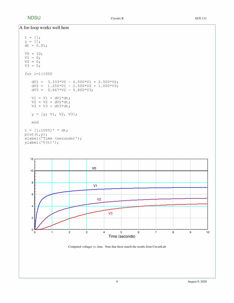
A for-loop works well here

t = [];y = [];dt = 0.01; V0 = 10;V1 = 0;V2 = 0;V3 = 0;

for i=1:1000 dV1 = 3.333*V0 - 6.500*V1 + 2.500*V2; dV2 = 1.250*V1 - 2.500*V2 + 1.000*V3; dV3 = 0.667*V2 - 0.800*V3;

V1 = V1 + dV1*dt; V2 = V2 + dV2*dt; V3 = V3 + dV3*dt;

y = [y; V1, V2, V3];

end

t = [1:1000]' * dt;plot(t,y);xlabel('Time (seconds)');ylabel('V(t)');

0 1 2 3 4 5 6 7 8 9 100

2

4

6

8

10

12

Time (seconds)

V0

V1

V2

V3

Computed votlages vs. time. Note that these match the results from CircuitLab

NDSU Circuits II ECE 111

6 August 9, 2020

Animation in MATLAB

You can also watch the voltages change vs. time. The trick is

Plot your function (the node voltages in this case), and

Insert a pause(0.01) command to pause the MATLAB program and display the current temperature

t = [];y = [];dt = 0.01;

V0 = 10; V1 = 0;V2 = 0;V3 = 0;

for i=1:1000 dV1 = 3.333*V0 - 6.500*V1 + 2.500*V2; dV2 = 1.250*V1 - 2.500*V2 + 1.000*V3; dV3 = 0.667*V2 - 0.800*V3;

V1 = V1 + dV1*dt; V2 = V2 + dV2*dt; V3 = V3 + dV3*dt;

plot([0:3], [V0; V1; V2; V3], '.-');

ylim([0,10]);

pause(0.01);

end

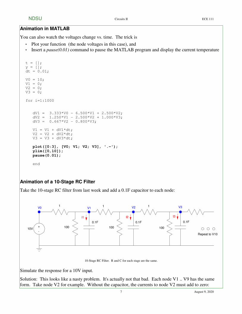
Animation of a 10-Stage RC Filter

Take the 10-stage RC filter from last week and add a 0.1F capacitor to each node:

+

-10V

1 1 1

100 100 100

0.1F 0.1F 0.1F

V0 V1 V2 V3

I1 I2 I3

Repeat to V10

10-Stage RC Filter. R and C for each stage are the same.

Simulate the response for a 10V input.

Solution: This looks like a nasty problem. It's actually not that bad. Each node V1 .. V9 has the same

form. Take node V2 for example. Without the capacitor, the currents to node V2 must add to zero:

NDSU Circuits II ECE 111

7 August 9, 2020

0 =

V1−V2

1 +

V3−V2

1 +

0−V2

100

With the capacitor, the current sums to the current to the capacitor

IC2= C2

dV2

dt=

V1−V2

1 +

V3−V2

1 +

0−V2

100

Simplifying and substituting C2 = 0.1F

dV2

dt= 10V1 − 20.1V2 + 10V3

This same pattern holds for V1 .. V9 (with V1 using the input Vin instead of V0)

The exception is node V10 where there is only one resistor attached:

IC10= C10

dV10

dt=

V9−V10

1 +

0−V10

100

dV10

dt= 10V9 − 10.1V10

This results in the matrix form of the dynamics being

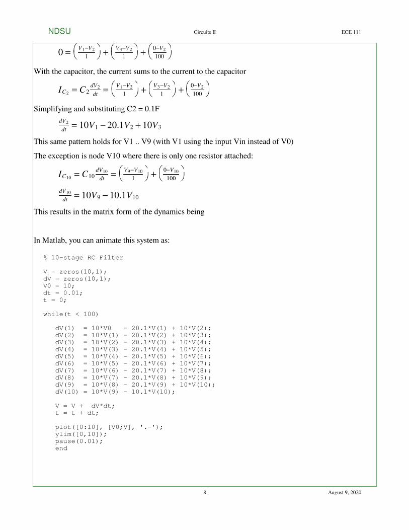
In Matlab, you can animate this system as:

% 10-stage RC Filter

V = zeros(10,1);dV = zeros(10,1);V0 = 10;dt = 0.01;t = 0;

while(t < 100)

dV(1) = 10*V0 - 20.1*V(1) + 10*V(2); dV(2) = 10*V(1) - 20.1*V(2) + 10*V(3); dV(3) = 10*V(2) - 20.1*V(3) + 10*V(4); dV(4) = 10*V(3) - 20.1*V(4) + 10*V(5); dV(5) = 10*V(4) - 20.1*V(5) + 10*V(6); dV(6) = 10*V(5) - 20.1*V(6) + 10*V(7); dV(7) = 10*V(6) - 20.1*V(7) + 10*V(8); dV(8) = 10*V(7) - 20.1*V(8) + 10*V(9); dV(9) = 10*V(8) - 20.1*V(9) + 10*V(10); dV(10) = 10*V(9) - 10.1*V(10);

V = V + dV*dt; t = t + dt;

plot([0:10], [V0;V], '.-'); ylim([0,10]); pause(0.01); end

NDSU Circuits II ECE 111

8 August 9, 2020

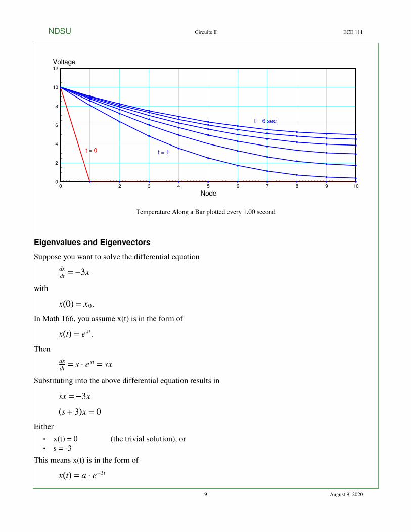
0 1 2 3 4 5 6 7 8 9 100

2

4

6

8

10

12

Node

Voltage

t = 0 t = 1

t = 6 sec

Temperature Along a Bar plotted every 1.00 second

Eigenvalues and Eigenvectors

Suppose you want to solve the differential equation

dx

dt= −3x

with

.x(0) = x0

In Math 166, you assume x(t) is in the form of

.x(t) = est

Then

dx

dt= s ⋅ est = sx

Substituting into the above differential equation results in

sx = −3x

(s + 3)x = 0

Either

x(t) = 0 (the trivial solution), or

s = -3

This means x(t) is in the form of

x(t) = a ⋅ e−3t

NDSU Circuits II ECE 111

9 August 9, 2020

Plug in the initial conditions and you get

x(t) = x0 ⋅ e−3t

This also works for matrices. If

X

.

= AX

then

X(t) = eAtX0

or in terms of eigenvalues and eigenvectors

X(t) = a1Λ1eλ1t + a2Λ2e

λ2t + ...a10Λ10eλ10t

where

is the ith eigenvector,Λ i

is the ith eigenvalue, andλ i

are constants determined by the initial condition.ai

Eigenvalues tell you how the system behaves

Eigenvectors tell you what behaves that way.

If X(0) is equal to an eigenvector, then only that one mode is excited.

The shape of x(t) remains the same (only one eigenvector is excited)

x(t) then goes to zero according to its eigenvalue.

If X(0) excites multiple eigenvectors, then X(t) will be the combination of all its eigenmodes.

NDSU Circuits II ECE 111

10 August 9, 2020

Example: Take for example, the 10-stage RC filter. In matrix form

V

.

1

V

.

2

V

.

3

V

.

4

V

.

5

V

.

6

V

.

7

V

.

8

V

.

9

V

.

10

=

−20.1 10 0 0 0 0 0 0 0 0

10 −20.1 10 0 0 0 0 0 0 0

0 10 −20.1 10 0 0 0 0 0 0

0 0 10 −20.1 10 0 0 0 0 0

0 0 0 10 −20.1 10 0 0 0 0

0 0 0 0 10 −20.1 10 0 0 0

0 0 0 0 0 10 −20.1 10 0 0

0 0 0 0 0 0 10 −20.1 10 0

0 0 0 0 0 0 0 10 −20.1 10

0 0 0 0 0 0 0 0 10 −10.1

V1

V2

V3

V4

V5

V6

V7

V8

V9

V10

+

10

0

0

0

0

0

0

0

0

0

V0

In Matlab, you can input this 10x10 system as

>> A = zeros(10,10);>> for i=1:9A(i,i) = -20.1;A(i,i+1) = 10;A(i+1,i) = 10;end>> A(10,10) = -10.1;>> A

-20.1000 10.0000 0 0 0 0 0 0 0 0 10.0000 -20.1000 10.0000 0 0 0 0 0 0 0 0 10.0000 -20.1000 10.0000 0 0 0 0 0 0 0 0 10.0000 -20.1000 10.0000 0 0 0 0 0 0 0 0 10.0000 -20.1000 10.0000 0 0 0 0 0 0 0 0 10.0000 -20.1000 10.0000 0 0 0 0 0 0 0 0 10.0000 -20.1000 10.0000 0 0 0 0 0 0 0 0 10.0000 -20.1000 10.0000 0 0 0 0 0 0 0 0 10.0000 -20.1000 10.0000 0 0 0 0 0 0 0 0 10.0000 -10.1000

The eigenvalues of the 10x10 matrix are:

>> eig(A)

-39.2115 -36.6248 -32.5698 -27.4068 -21.5946 -15.6496 -10.1000 -5.4390 -2.0806 -0.3234

Eigenvalues tell you how the system behaves.

There is a fast mode which decays as

x(t) = e−39.21t

NDSU Circuits II ECE 111

11 August 9, 2020

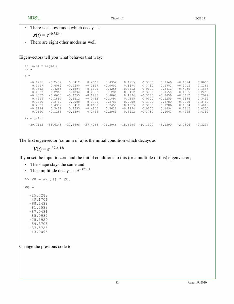
There is a slow mode which decays as

x(t) = e−0.3234t

There are eight other modes as well

Eigenvectors tell you what behaves that way:

>> [a,b] = eig(A);>> a

a =

-0.1286 -0.2459 0.3412 0.4063 0.4352 0.4255 0.3780 0.2969 -0.1894 0.0650 0.2459 0.4063 -0.4255 -0.2969 -0.0650 0.1894 0.3780 0.4352 -0.3412 0.1286 -0.3412 -0.4255 0.1894 -0.1894 -0.4255 -0.3412 -0.0000 0.3412 -0.4255 0.1894 0.4063 0.2969 0.1894 0.4352 0.1286 -0.3412 -0.3780 0.0650 -0.4255 0.2459 -0.4352 -0.0650 -0.4255 -0.1286 0.4063 0.1894 -0.3780 -0.2459 -0.3412 0.2969 0.4255 -0.1894 0.3412 -0.3412 -0.1894 0.4255 0.0000 -0.4255 -0.1894 0.3412 -0.3780 0.3780 0.0000 0.3780 -0.3780 -0.0000 0.3780 -0.3780 -0.0000 0.3780 0.2969 -0.4352 -0.3412 0.0650 0.2459 -0.4255 0.3780 -0.1286 0.1894 0.4063 -0.1894 0.3412 0.4255 -0.4255 0.3412 -0.1894 0.0000 0.1894 0.3412 0.4255 0.0650 -0.1286 -0.1894 0.2459 -0.2969 0.3412 -0.3780 0.4063 0.4255 0.4352

>> eig(A)'

-39.2115 -36.6248 -32.5698 -27.4068 -21.5946 -15.6496 -10.1000 -5.4390 -2.0806 -0.3234

The first eigenvector (column of a) is the initial condition which decays as

V(t) = e−39.2115t

If you set the input to zero and the initial conditions to this (or a multiple of this) eigenvector,

The shape stays the same and

The amplitude decays as e−39.21t

>> V0 = a(:,1) * 200

V0 =

-25.7283 49.1706 -68.2438 81.2533 -87.0431 85.0987 -75.5929 59.3703 -37.8725 13.0095

Change the previous code to

NDSU Circuits II ECE 111

12 August 9, 2020

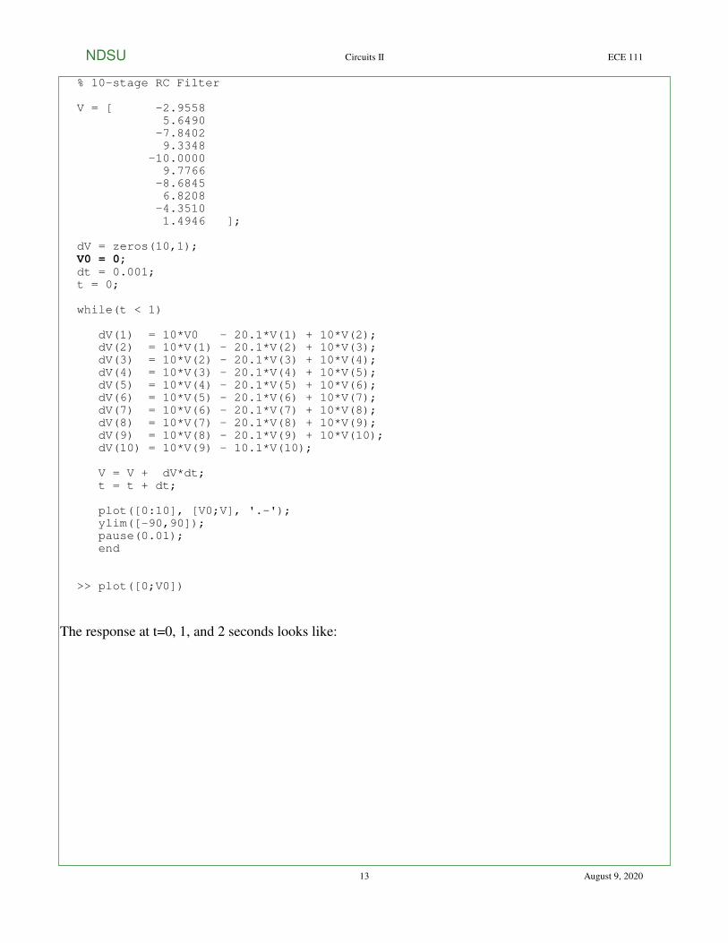
% 10-stage RC Filter

V = [ -2.9558 5.6490 -7.8402 9.3348 -10.0000 9.7766 -8.6845 6.8208 -4.3510 1.4946 ];

dV = zeros(10,1);

V0 = 0;

dt = 0.001;t = 0;

while(t < 1)

dV(1) = 10*V0 - 20.1*V(1) + 10*V(2); dV(2) = 10*V(1) - 20.1*V(2) + 10*V(3); dV(3) = 10*V(2) - 20.1*V(3) + 10*V(4); dV(4) = 10*V(3) - 20.1*V(4) + 10*V(5); dV(5) = 10*V(4) - 20.1*V(5) + 10*V(6); dV(6) = 10*V(5) - 20.1*V(6) + 10*V(7); dV(7) = 10*V(6) - 20.1*V(7) + 10*V(8); dV(8) = 10*V(7) - 20.1*V(8) + 10*V(9); dV(9) = 10*V(8) - 20.1*V(9) + 10*V(10); dV(10) = 10*V(9) - 10.1*V(10);

V = V + dV*dt; t = t + dt;

plot([0:10], [V0;V], '.-'); ylim([-90,90]); pause(0.01); end

>> plot([0;V0])

The response at t=0, 1, and 2 seconds looks like:

NDSU Circuits II ECE 111

13 August 9, 2020

0 1 2 3 4 5 6 7 8 9 10-12

-10

-8

-6

-4

-2

0

2

4

6

8

10

12

Node

Voltage

t = 0

Noce voltages plotted every X(t) plotted every 0.02 seconds.

Note that

The shape of the curve remains the same as defined by the eigenvector that's excited

This mode decays very quickly as

V(t) = V0e−39.21t

If you excite the slow eigenvector instead, the system decays very slowly. The slow eigenvector is

>> a(:,10)/max(abs(a(:,10))*10

1.4946 2.9558 4.3510 5.6490 6.8208 7.8402 8.6845 9.3348 9.7766 10.0000

If this is the initial condition then the response is

NDSU Circuits II ECE 111

14 August 9, 2020

0 1 2 3 4 5 6 7 8 9 100

2

4

6

8

10

12

Node

Voltage

t = 0

V(t) plotted every 1.00 second

Note that

The shape of the curve remains the same as defined by the eigenvector that's excited

This mode decays very slowly as

V(t) = V0e−0.33234t

If you have a random initial condition, then all ten eigenmodes will be excited. Quickly, the fast modes

die out. All you're left with then is the slow mode.

For example, let the initial condition be:

>> V0 = 10*rand(10,1)

NDSU Circuits II ECE 111

15 August 9, 2020

0 1 2 3 4 5 6 7 8 9 100

2

4

6

8

10

12

Node

Voltage

t = 0

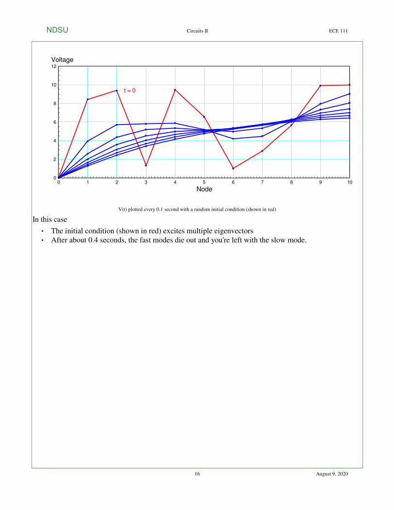
V(t) plotted every 0.1 second with a random initial condition (shown in red)

In this case

The initial condition (shown in red) excites multiple eigenvectors

After about 0.4 seconds, the fast modes die out and you're left with the slow mode.

NDSU Circuits II ECE 111

16 August 9, 2020