Multivariate Time Series: VAR(p) Processes and

Models

A VAR(p) model, for p > 0 is

Xt = φ0 + Φ1Xt−1 + · · · + ΦpXt−p + At,

where Xt, φ0, and Xt−i are k-vectors, Φ1, . . . , Φp are k×k matrices,

with Φp 6= 0, and {At} is a sequence of serially uncorrelated

k-vectors with 0 mean and constant positive definite variance-

covariance matrix Σ.

We also can write this using the back-shift operator as

(I − Φ1B − · · · − ΦpBp)Xt = φ0 + At,

or

Φ(B)Xt = φ0 + At,

1

Companion Matrix

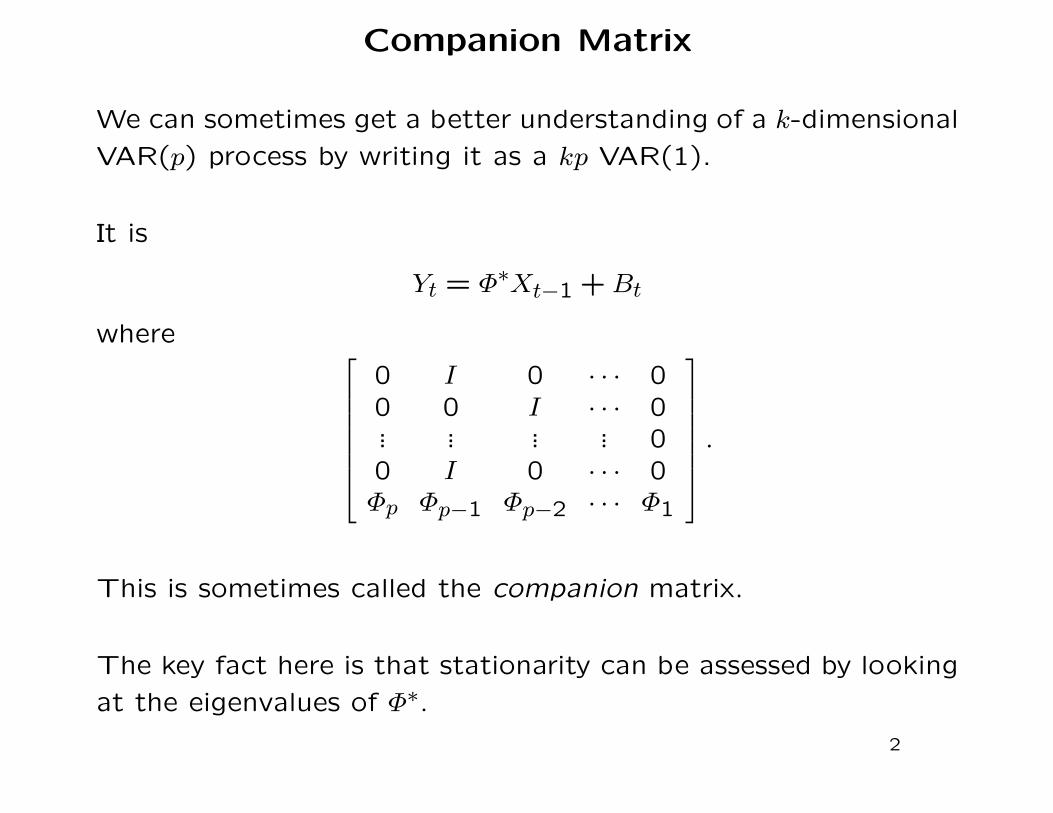
We can sometimes get a better understanding of a k-dimensional

VAR(p) process by writing it as a kp VAR(1).

It is

Yt = Φ∗Xt−1 + Bt

where

0 I 0 · · · 00 0 I · · · 0... ... ... ... 00 I 0 · · · 0Φp Φp−1 Φp−2 · · · Φ1

.

This is sometimes called the companion matrix.

The key fact here is that stationarity can be assessed by looking

at the eigenvalues of Φ∗.

2

Number of Terms in Time Series Models

The two common general types of time series models incorporate

past history either through linear combinations of past observa-

tions (AR) or of previous errors (shocks) in the system (MA).

To use either type of model, we need to decide on the order.

For an AR model, we do that by using a sequence of partial

models.

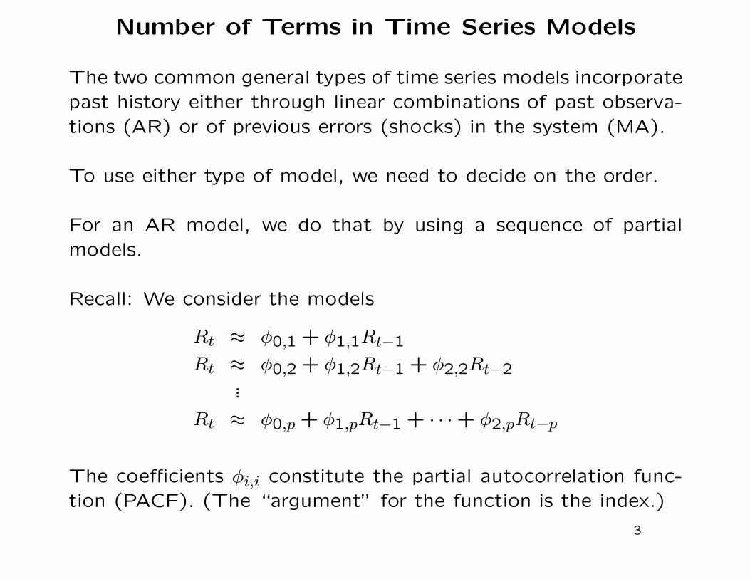
Recall: We consider the models

Rt ≈ φ0,1 + φ1,1Rt−1

Rt ≈ φ0,2 + φ1,2Rt−1 + φ2,2Rt−2...

Rt ≈ φ0,p + φ1,pRt−1 + · · · + φ2,pRt−p

The coefficients φi,i constitute the partial autocorrelation func-

tion (PACF). (The “argument” for the function is the index.)

3

The Partial Autocorrelation Function (PACF) in

AR Models

The PACF is useful for an AR model because we can “partial

out” the dependence.

Consider AR(1): Rt = φRt−1 + At.

We have γ(2) = φ2γ(0) for Rt and Rt−2.

Could we get a covariance of something to go to 0 at lag 2?

Consider Rt − φRt−1 and Rt−2 − φRt−1. The covariance is 0.

This is the idea behind the PACF; for Rt and Rt+h, regress each

on the Rk’s between them.

The important result is that the PACF in an AR(p) model is

0 beyond lag p; that is φp+1,p+1 = 0; hence, we can use it to

identify p.

4

The Partial Autocorrelation Function (PACF) in

AR Models

The question is how to use the sample PACF.

Often, since after all, we use it to build a model, we just use

simple graphs to decide at what order the sample PACF has died

off.

More formally, if the errors in the AR(p) model are iid with

mean 0, then the sample PACFs beyond p are asymptotically

iid N(0,1/n).

5

Number of Terms in a VAR(p) Model

We use similar ideas to determine the p in a VAR(p) model.

Instead of scalar partial correlations, however, we have partial

covariance matrices.

It’s a little harder even to get started.

We take a parametric approach using a multivariate normal dis-

tribution.

Residuals from a partial true model have a PDF of the form

f(r) =1

(2π)k/2|Σ|1/2exp

((r − µr)

TΣ−1(r − µr)/2)

.

6

Sequential Tests for Φj = 0 in a VAR(p) Model

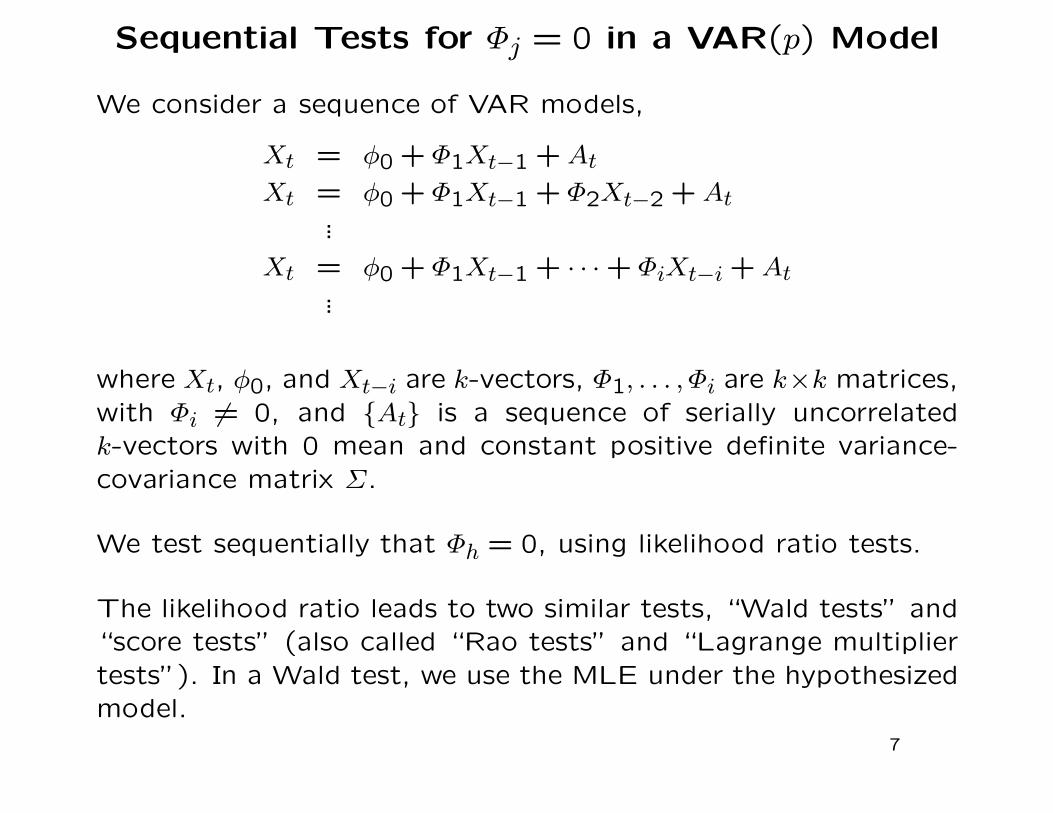
We consider a sequence of VAR models,

Xt = φ0 + Φ1Xt−1 + At

Xt = φ0 + Φ1Xt−1 + Φ2Xt−2 + At...

Xt = φ0 + Φ1Xt−1 + · · · + ΦiXt−i + At...

where Xt, φ0, and Xt−i are k-vectors, Φ1, . . . , Φi are k×k matrices,

with Φi 6= 0, and {At} is a sequence of serially uncorrelated

k-vectors with 0 mean and constant positive definite variance-

covariance matrix Σ.

We test sequentially that Φh = 0, using likelihood ratio tests.

The likelihood ratio leads to two similar tests, “Wald tests” and

“score tests” (also called “Rao tests” and “Lagrange multiplier

tests”). In a Wald test, we use the MLE under the hypothesized

model.

7

Sequential Tests for Φj = 0 in a VAR(p) Model

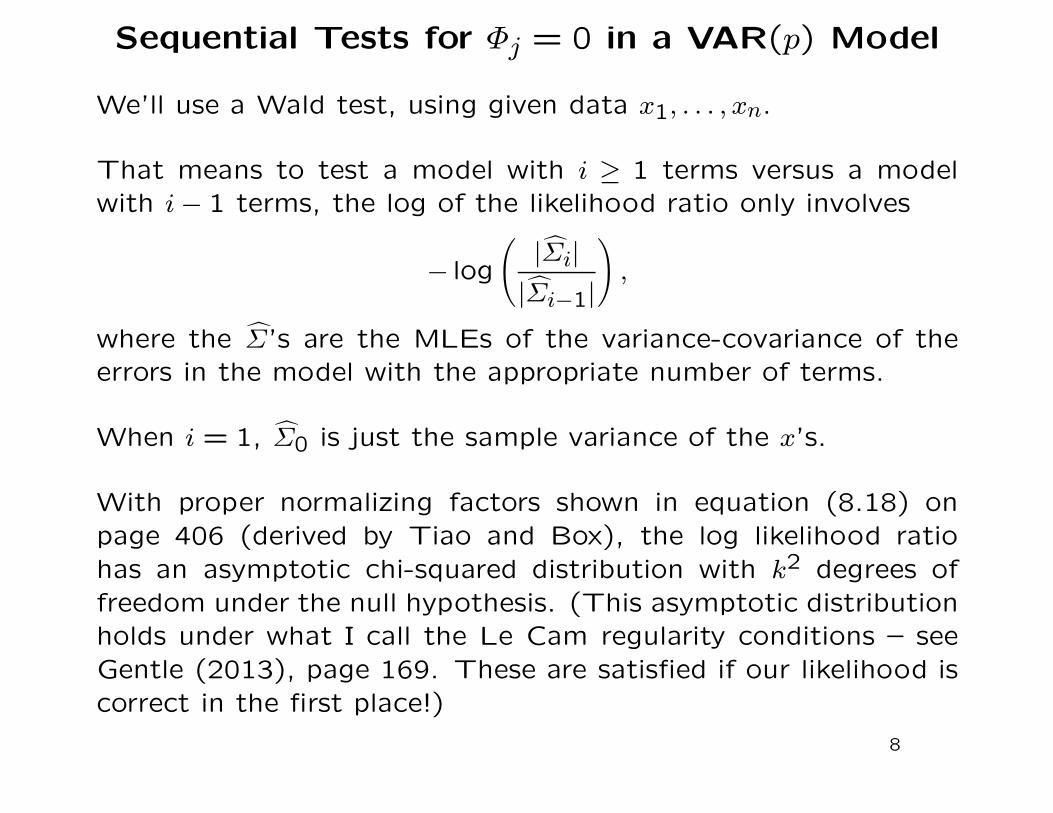
We’ll use a Wald test, using given data x1, . . . , xn.

That means to test a model with i ≥ 1 terms versus a model

with i − 1 terms, the log of the likelihood ratio only involves

− log

(|Σ̂i|

|Σ̂i−1|

),

where the Σ̂’s are the MLEs of the variance-covariance of the

errors in the model with the appropriate number of terms.

When i = 1, Σ̂0 is just the sample variance of the x’s.

With proper normalizing factors shown in equation (8.18) on

page 406 (derived by Tiao and Box), the log likelihood ratio

has an asymptotic chi-squared distribution with k2 degrees of

freedom under the null hypothesis. (This asymptotic distribution

holds under what I call the Le Cam regularity conditions – see

Gentle (2013), page 169. These are satisfied if our likelihood is

correct in the first place!)

8

Sequential Tests for Φj = 0 in a VAR(p) Model

We test

H0 : Φ1 = 0 versus H1 : Φ1 6= 0.

What next?

In practice, whether or not we reject, we may try H0 : Φ2 = 0,

but usually we don’t – we proceed to the next model only if we

reject the preceding hypothesis.

I am not sure whether there is an R function that does these

tests directly, but the output of VAR in the var package can easily

be used to compute the statistic.

9

The ARCH Effect in a VAR(p) Model

An extension to the VAR model allows for the volatility to vary

as in an ARCH or GARCH model.

The R function serial.test in the var package computes the

portmanteau test statistic for the ARCH effect (at least if the

model is VAR+ARCH).

10

Forecasting with a VAR(p) Model

Forecasting with a VAR(p) model is similar to the same thing in

a univariate model.

Given xt, . . . , xt−p+1, the 1-step-ahead forecast at time t is

Xt(1) = φ0 +p∑

i=1

ΦiXt+1−i,

and the forecast error is At+1.

Substituting, we get the 2-step-ahead forecast at time t as

Xt(2) = φ0 + Φ1Xt(1) +p∑

i=2

ΦiXt+2−i,

and the forecast error is At+2 + Φ1At+1.

11

Impulse Response Function

We can also express a causal VAR(p) as an infinite moving av-

erage model model just as we did with a univariate model:

Xt = θ0 + At + Ψ1At−1 + Ψ2At−2 + · · ·

The coefficient matrices in such an infinite MA model are called

impulse response functions.

What’s “causal”?

12

Vector Moving-Average or VMA(q) Models and

VARMA(p, q) Models

The vector moving-average or VMA(q) model is the obvious ex-

tension of the univariate MA model.

We can write it as

Xt = θ0 + At − Θ1At−1 − · · · − ΘqAt−q

or

Xt = θ0 + Θ(B)At.

The differences between a VMA and an MA are similar to the

differences between a VAR and an AR.

Also, just as we combine an AR model and an MA model, we

combine a VAR and a VMA to get a vector ARMA or VARMA(p, q)

model.

13

Marginal Models of Components of VMA(q)

Models

The marginal models of a VMA(q) model are just MA(q) models.

We see this because the cross-correlation matrix of Xt vanishes

after lag q, and so we can write Xit as

Xit = θi0 +q∑

j=1

θi,jBi,t−j,

where {Bi,t−j} is a sequence of uncorrelated random variable with

0 mean and constant variance.

14

Marginal Models of Components of VAR(p)

Models

One approach to studying the marginal components of VAR(p)

models is by use of the structural equations. These are formed

by diagaonalizing the variance-covariance matrix of At, as we

discussed last week for a VAR(p) model. This approach shows

the concurrent relationships of one component to all the others.

Another approach is to obtain explicit representations of all of

the component series as AR models.

We can do this if we can diagonalize the AR polynomial coeffi-

cient matrix in a VAR(p) model.

15

Marginal Models of Components and

Diagonalizing Matrices

Some technical notes are in order here. A nonnegative definite matrix canalways be diagonalized by a Cholesky decomposition, but not all square ma-trices can be diagonalized. A matrix that can be diagonalized is called aregular matrix. (See Gentle, 2007, pages 116 and following, for conditionsand general discussion of the problem.)

One general method of diagonalizing a regular matrix A is to use the matrixV whose columns are linearly independent eigenvectors of A and C is thediagonal matrix whose elements are the eigenvalues of A. This requires bothpremultiplication and postmultiplication of A, and if the matrix is not of fullrank, requires some rearrangement of the rows and columns.

16

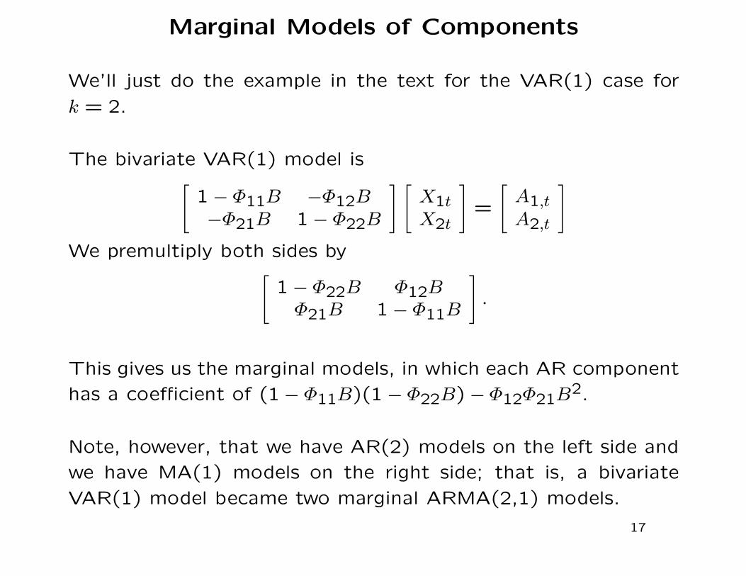
Marginal Models of Components

We’ll just do the example in the text for the VAR(1) case for

k = 2.

The bivariate VAR(1) model is[

1 − Φ11B −Φ12B−Φ21B 1 − Φ22B

] [X1tX2t

]=

[A1,tA2,t

]

We premultiply both sides by[

1 − Φ22B Φ12BΦ21B 1 − Φ11B

].

This gives us the marginal models, in which each AR component

has a coefficient of (1 − Φ11B)(1 − Φ22B) − Φ12Φ21B2.

Note, however, that we have AR(2) models on the left side and

we have MA(1) models on the right side; that is, a bivariate

VAR(1) model became two marginal ARMA(2,1) models.

17

Marginal Models of Components

This idea generalizes (with a lot of tedious algebra).

A k-variate VAR(p) model yields k ARMA(kp, (k − 1)p) models.

The VMA(q) part of the original VARMA may add up to q ad-

dition MA components. In general, however, the number of MA

components is min((k − 1)p, q).

We next consider some other ways that decomposing a VAR(p)

model can lead to new insights about the process in some cases.

This is the case where we have cointegration.

18

Unit-Root Nonstationarity

Many economic time series exhibit either (apparent) random walk

behavior,

Pt = Pt−1 + At,

or random walk with a drift behavior,

Pt = µ + Pt−1 + At,

where {At} is iid with variance σ2A.

Either of these processes has unit-root nonstationarity.

These processes can be made stationary by differencing; that is,

the series is “integrated”.

We speak of integrated series of order d, and denote as I(d), if

d differences result in a stationary process.

Notice the effects of the nonstationarity.

19

Simple Random Walk Process

In the simple random walk process, the k-step ahead forecast is

P̂t(k) = E(Pt+k|pt, pt−1, . . . , p0) = pt.

It is not mean reverting.

The forecast error is

et(k) = at+k + · · · + at+1

Its variance is

V(Et(k)) = kσ2A.

The forecast has no value.

20

Random Walk Process with Drift

In the simple random walk process, the k-step ahead forecast is

P̂t(k) = E(Pt+k|pt, pt−1, . . . , p0) = kµ + p0.

It is not mean reverting.

The conditional variance of Pt is tσ2A, which grows without bound.

I should mention one more type of nonstationary process. It is

the trend-stationary process,

Pt = α0 + α1t + At.

Notice that this process is not stationary because of its mean;

its variance, however, is time invariant.

This process can be made stationary by detrending, that is, by

subtracting βt.

21

Spurious Regressions

First, consider two trend-stationary processes,

Yt = α0 + α1t + At

and

Xt = δ0 + δ1t + Bt,

that have nothing to do with each other (i.e., everything is “in-

dependent”).

Now, consider the regression of Yt on Xt:

Yt = β0 + β1Xt + εt= β0 + β1(δ0 + δ1t + Bt) + εt= γ0 + (β1δ1)t + εt.

The regression test will probably be significant.

This results from the trends.

It is “spurious”, however. Everybody knows this.

22

Spurious Regressions

Next, consider two random walks,

Yt = yt−1 + At

and

Xt = xt−1 + Bt,

that have nothing to do with each other (i.e., everything is “inde-

pendent”). For simplicity, assume that At and Bt are iid N(0,1).

Now, consider the regression of Yt on Xt (without intercept):

Yt = βXt + εt.

We see that

β = Cov(Yt, Xt)/V(Xt)

and

εt ∼ N(0, t).

23

Spurious Regressions of Random Walks

Granger and Newbold, in a very famous Monte Carlo study in

1974, found that the standard t test of H0 : β = 0 rejected 76%

of the time.

This example is very different from the spurious regressions of

one trend-stationary series on another.

The problem here is unit-root nonstationarity.

24

Spurious Regressions of Random Walks:

A Technical Aside

Consider a regression model of the form Yt = βxt + εt, with the

usual assumption of 0 correlations between all εt and V(εt) = σ2.

What about the relationship between xt and εt?

The asymptotic properties (relating to normality) will hold if xt

and εt are independent.

This is OK if xt is a constant.

What about if xt is a random variable?

This happens all the time in financial applications.

In these applications, however, we cannot assume that xt and εtare independent.

Can we find a weaker condition?

25

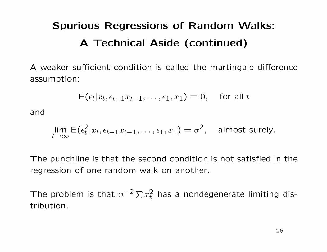
Spurious Regressions of Random Walks:

A Technical Aside (continued)

A weaker sufficient condition is called the martingale difference

assumption:

E(εt|xt, εt−1xt−1, . . . , ε1, x1) = 0, for all t

and

limt→∞

E(ε2t |xt, εt−1xt−1, . . . , ε1, x1) = σ2, almost surely.

The punchline is that the second condition is not satisfied in the

regression of one random walk on another.

The problem is that n−2∑x2t has a nondegenerate limiting dis-

tribution.

26

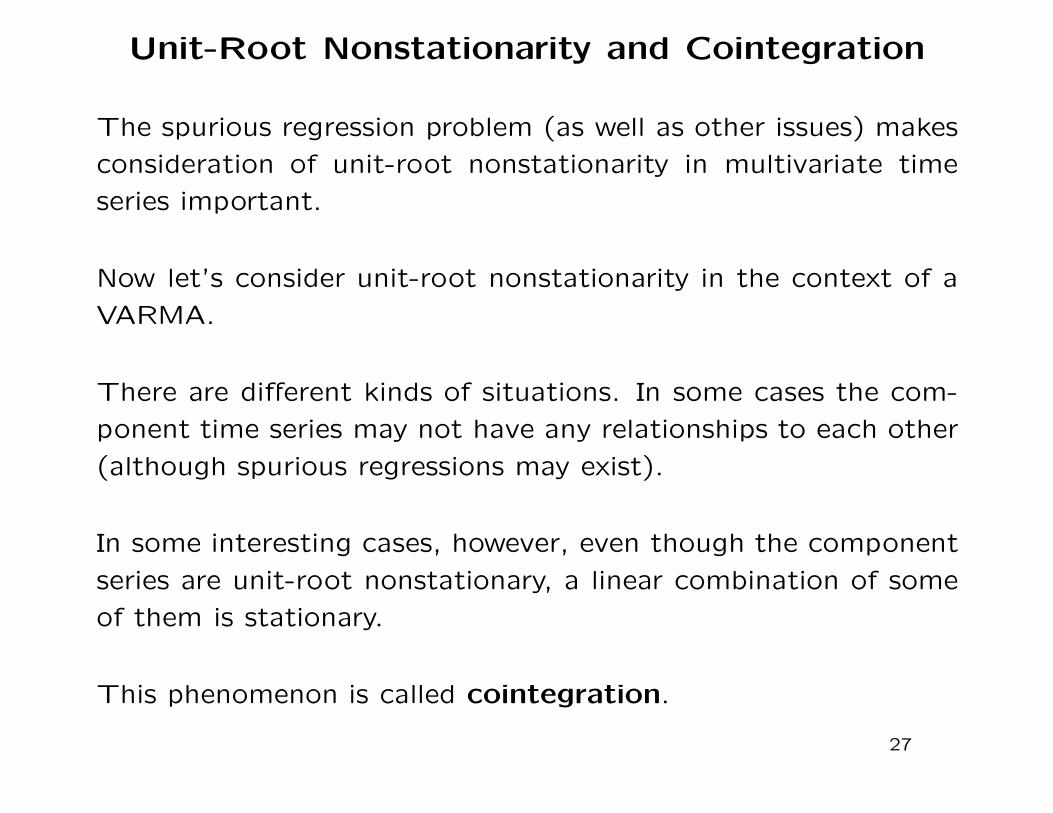
Unit-Root Nonstationarity and Cointegration

The spurious regression problem (as well as other issues) makes

consideration of unit-root nonstationarity in multivariate time

series important.

Now let’s consider unit-root nonstationarity in the context of a

VARMA.

There are different kinds of situations. In some cases the com-

ponent time series may not have any relationships to each other

(although spurious regressions may exist).

In some interesting cases, however, even though the component

series are unit-root nonstationary, a linear combination of some

of them is stationary.

This phenomenon is called cointegration.

27

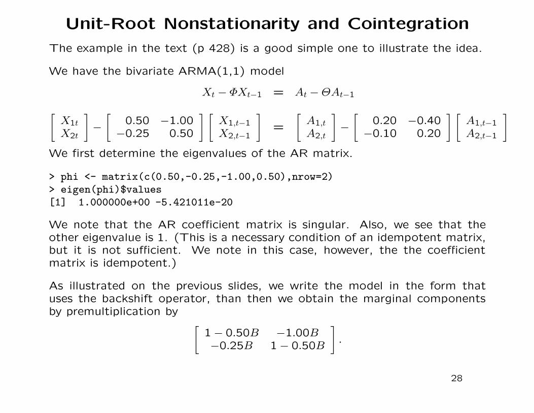
Unit-Root Nonstationarity and Cointegration

The example in the text (p 428) is a good simple one to illustrate the idea.

We have the bivariate ARMA(1,1) model

Xt − ΦXt−1 = At − ΘAt−1

[X1t

X2t

]−

[0.50 −1.00

−0.25 0.50

] [X1,t−1

X2,t−1

]=

[A1,t

A2,t

]−

[0.20 −0.40

−0.10 0.20

] [A1,t−1

A2,t−1

]

We first determine the eigenvalues of the AR matrix.

> phi <- matrix(c(0.50,-0.25,-1.00,0.50),nrow=2)> eigen(phi)$values[1] 1.000000e+00 -5.421011e-20

We note that the AR coefficient matrix is singular. Also, we see that theother eigenvalue is 1. (This is a necessary condition of an idempotent matrix,but it is not sufficient. We note in this case, however, the the coefficientmatrix is idempotent.)

As illustrated on the previous slides, we write the model in the form thatuses the backshift operator, than then we obtain the marginal componentsby premultiplication by

[1 − 0.50B −1.00B−0.25B 1 − 0.50B

].

28

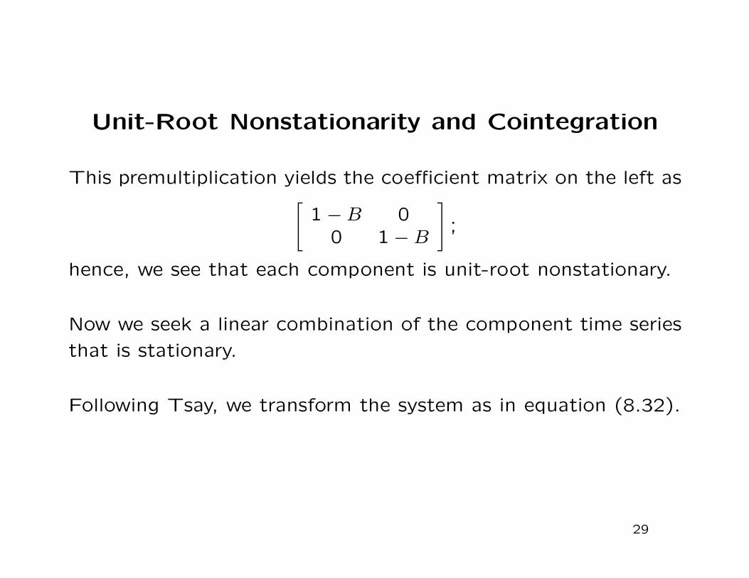
Unit-Root Nonstationarity and Cointegration

This premultiplication yields the coefficient matrix on the left as[

1 − B 00 1 − B

];

hence, we see that each component is unit-root nonstationary.

Now we seek a linear combination of the component time series

that is stationary.

Following Tsay, we transform the system as in equation (8.32).

29

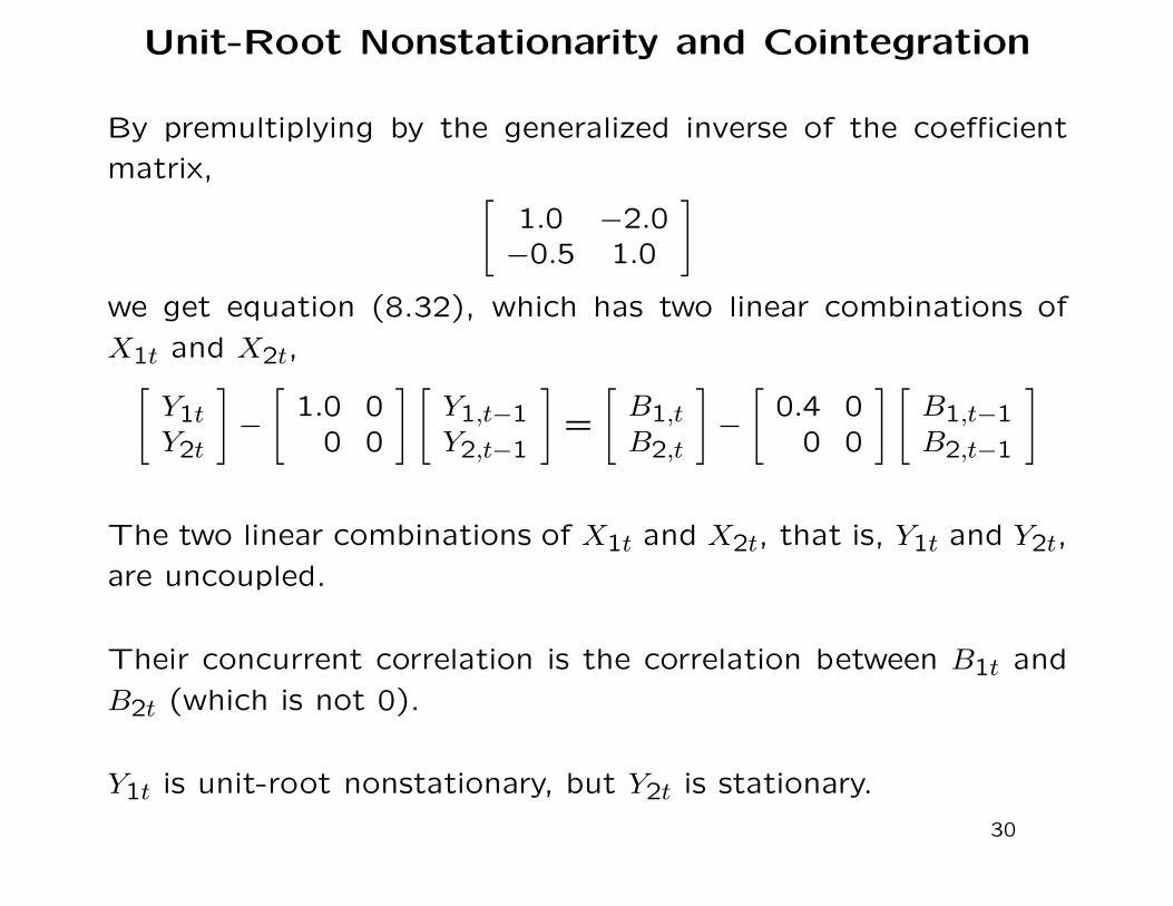
Unit-Root Nonstationarity and Cointegration

By premultiplying by the generalized inverse of the coefficient

matrix,[

1.0 −2.0−0.5 1.0

]

we get equation (8.32), which has two linear combinations of

X1t and X2t,[

Y1tY2t

]−

[1.0 0

0 0

] [Y1,t−1

Y2,t−1

]=

[B1,tB2,t

]−

[0.4 0

0 0

] [B1,t−1

B2,t−1

]

The two linear combinations of X1t and X2t, that is, Y1t and Y2t,

are uncoupled.

Their concurrent correlation is the correlation between B1t and

B2t (which is not 0).

Y1t is unit-root nonstationary, but Y2t is stationary.

30

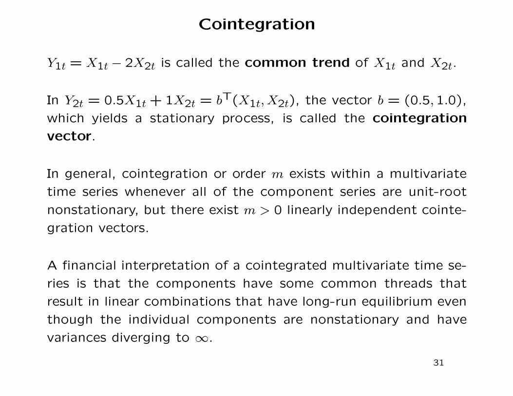
Cointegration

Y1t = X1t − 2X2t is called the common trend of X1t and X2t.

In Y2t = 0.5X1t + 1X2t = bT(X1t, X2t), the vector b = (0.5,1.0),

which yields a stationary process, is called the cointegration

vector.

In general, cointegration or order m exists within a multivariate

time series whenever all of the component series are unit-root

nonstationary, but there exist m > 0 linearly independent cointe-

gration vectors.

A financial interpretation of a cointegrated multivariate time se-

ries is that the components have some common threads that

result in linear combinations that have long-run equilibrium even

though the individual components are nonstationary and have

variances diverging to ∞.

31

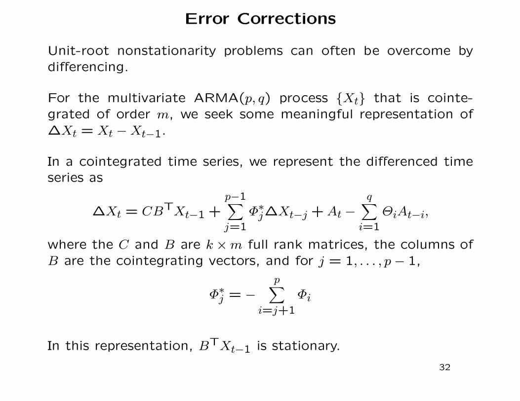
Error Corrections

Unit-root nonstationarity problems can often be overcome by

differencing.

For the multivariate ARMA(p, q) process {Xt} that is cointe-

grated of order m, we seek some meaningful representation of

∆Xt = Xt − Xt−1.

In a cointegrated time series, we represent the differenced time

series as

∆Xt = CBTXt−1 +p−1∑

j=1

Φ∗j∆Xt−j + At −

q∑

i=1

ΘiAt−i,

where the C and B are k × m full rank matrices, the columns of

B are the cointegrating vectors, and for j = 1, . . . , p − 1,

Φ∗j = −

p∑

i=j+1

Φi

In this representation, BTXt−1 is stationary.

32

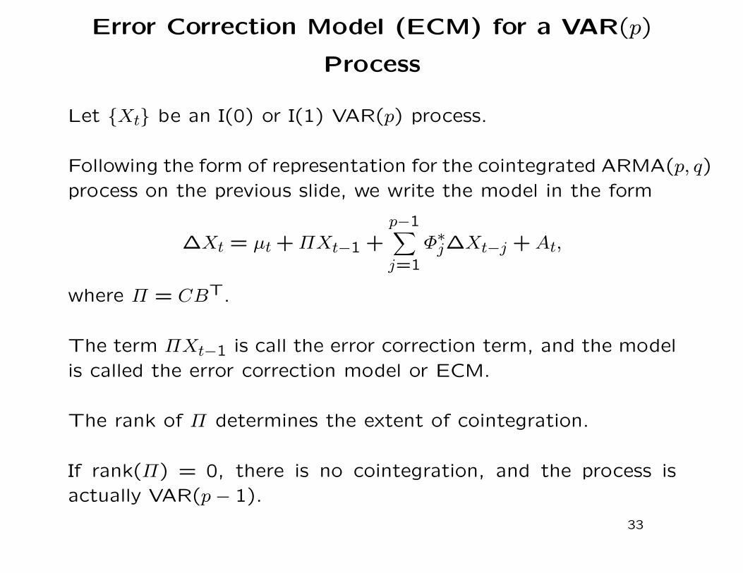
Error Correction Model (ECM) for a VAR(p)

Process

Let {Xt} be an I(0) or I(1) VAR(p) process.

Following the form of representation for the cointegrated ARMA(p, q)

process on the previous slide, we write the model in the form

∆Xt = µt + ΠXt−1 +p−1∑

j=1

Φ∗j∆Xt−j + At,

where Π = CBT.

The term ΠXt−1 is call the error correction term, and the model

is called the error correction model or ECM.

The rank of Π determines the extent of cointegration.

If rank(Π) = 0, there is no cointegration, and the process is

actually VAR(p − 1).

33

If rank(Π) = k, that is the matrix is full-rank, there is no coin-

tegration, and the process is just VAR(p).

If < 0rank(Π) = m < k, there is cointegration of order m.

Johansen’s Test

To test for cointegration in a nominal VAR(p) process is essen-

tially to test the rank of Π.

There is a likelihood ratio test for this, called Johansen’s test.

It is in the R function ca.jo in the urca package.

34

Cointegrated Financial Time Series

The only way to receive returns uniformly above a risk-adjusted

rate is by arbitrage.

In a fair and stable market, there is no arbitrage.

Whenever cointegrated time series exist, there is often the pos-

sibility that the two series do not reflect true value.

An example is pairs trading.

35