Motivation and main results.

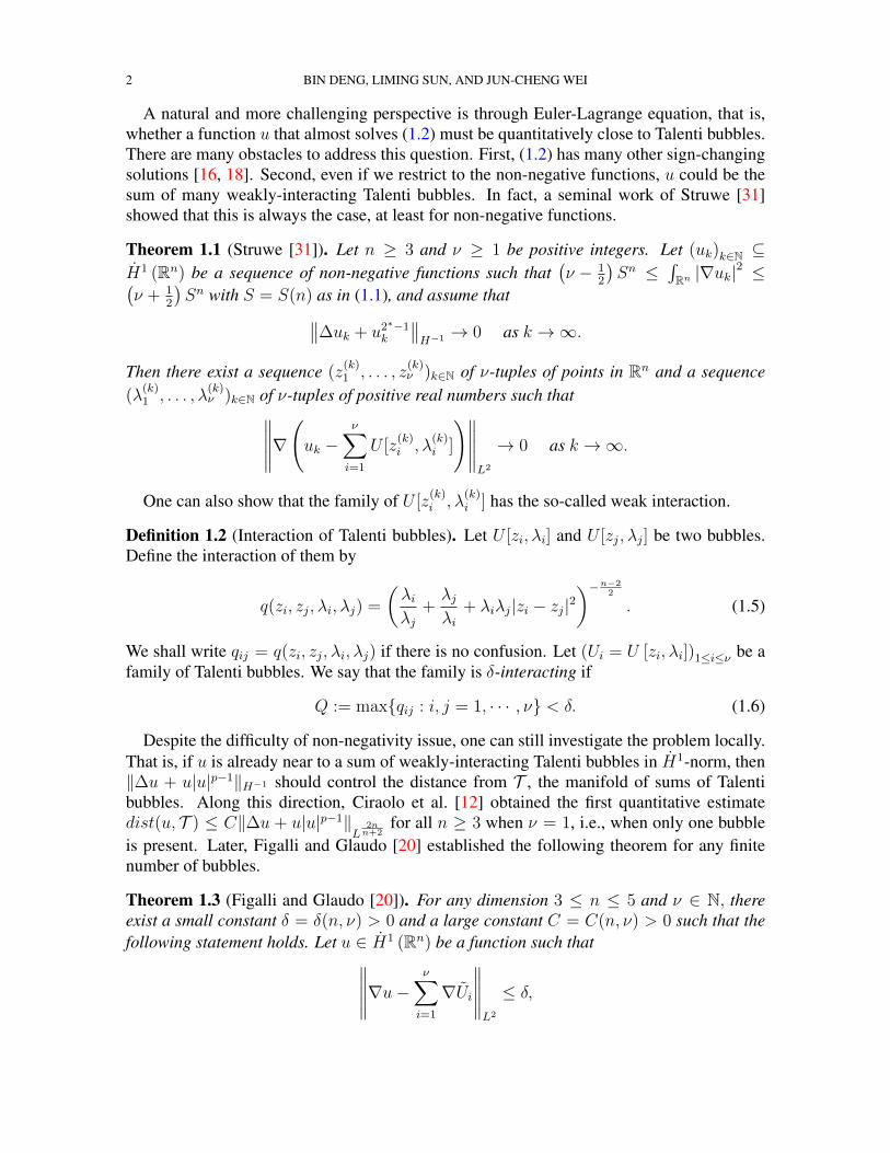
SHARP QUANTITATIVE ESTIMATES OF STRUWE’S DECOMPOSITION

BIN DENG, LIMING SUN, AND JUN-CHENG WEI

ABSTRACT. Suppose u ∈ H1(Rn). In a seminal work, Struwe proved that if u ≥ 0 andΓ(u) := ‖∆u + u

n+2n−2 ‖H−1 → 0 then dist(u, T ) → 0, where dist(u, T ) denotes the

H1(Rn)-distance of u from the manifold of sums of Talenti bubbles. Ciraolo, Figalli andMaggi obtained the first quantitative version of Struwe’s decomposition with one bubble inall dimensions, namely dist(u, T ) ≤ CΓ(u). For Struwe’s decomposition with two or morebubbles, Figalli and Glaudo showed a striking dimensional dependent quantitative estimate,namely dist(u, T ) ≤ CΓ(u) when 3 ≤ n ≤ 5 while this is false for n ≥ 6. In this paper, weshow that

dist(u, T ) ≤ C

Γ(u) |log Γ(u)|

12 if n = 6,

|Γ(u)|n+2

2(n−2) if n ≥ 7.

Furthermore, we show that this inequality is sharp.

1. INTRODUCTION

1.1. Motivation and main results. The Sobolev inequality with exponent 2 states that, forany n ≥ 3 and any u ∈ H1 (Rn) := D1,2 (Rn), it holds that

S‖u‖L2∗ ≤ ‖∇u‖L2 , (1.1)

where 2∗ = 2nn−2

and S = S(n) is a dimensional constant.It is well-known that the Euler-Lagrange equation of (1.1), i.e., critical points of Sobolev

inequality, up to scaling, is given by

∆u+ |u|p−1u = 0 in Rn. (1.2)

Throughout this paper, we denote p = n+2n−2

. By Caffarelli et al. [9] and Gidas et al. [24], it isknown that all the positive solutions are Talenti bubbles [32], i.e.

U [z, λ](x) := (n(n− 2))n−24

(λ

1 + λ2|x− z|2

)n−22

. (1.3)

These are all the minimizers of the Sobolev inequality, up to scaling. There are many inter-ests regarding to the stability of (1.1). From the perspective of discrepancy in the Sobolevinequality, Bianchi and Egnell [6] gave a quantitative estimate near the minimizers, that is

infz∈Rn,λ>0,α∈R

‖∇(u− αU [z, λ])‖2L2 ≤ C(n)

(‖∇u‖2

L2 − S2‖u‖2L2∗). (1.4)

Date: July 25, 2021 (Last Typeset).2010 Mathematics Subject Classification. Primary 35A23, 26D10; Secondary 35B35, 35J20.Key words and phrases. Sobolev inequality, stability, quantitative estimates, Struwe’s decomposition, re-

duction method.1

2 BIN DENG, LIMING SUN, AND JUN-CHENG WEI

A natural and more challenging perspective is through Euler-Lagrange equation, that is,whether a function u that almost solves (1.2) must be quantitatively close to Talenti bubbles.There are many obstacles to address this question. First, (1.2) has many other sign-changingsolutions [16, 18]. Second, even if we restrict to the non-negative functions, u could be thesum of many weakly-interacting Talenti bubbles. In fact, a seminal work of Struwe [31]showed that this is always the case, at least for non-negative functions.

Theorem 1.1 (Struwe [31]). Let n ≥ 3 and ν ≥ 1 be positive integers. Let (uk)k∈N ⊆H1 (Rn) be a sequence of non-negative functions such that

(ν − 1

2

)Sn ≤

∫Rn |∇uk|

2 ≤(ν + 1

2

)Sn with S = S(n) as in (1.1), and assume that∥∥∆uk + u2∗−1

k

∥∥H−1 → 0 as k →∞.

Then there exist a sequence (z(k)1 , . . . , z

(k)ν )k∈N of ν-tuples of points in Rn and a sequence

(λ(k)1 , . . . , λ

(k)ν )k∈N of ν-tuples of positive real numbers such that∥∥∥∥∥∇

(uk −

ν∑i=1

U [z(k)i , λ

(k)i ]

)∥∥∥∥∥L2

→ 0 as k →∞.

One can also show that the family of U [z(k)i , λ

(k)i ] has the so-called weak interaction.

Definition 1.2 (Interaction of Talenti bubbles). Let U [zi, λi] and U [zj, λj] be two bubbles.Define the interaction of them by

q(zi, zj, λi, λj) =

(λiλj

+λjλi

+ λiλj|zi − zj|2)−n−2

2

. (1.5)

We shall write qij = q(zi, zj, λi, λj) if there is no confusion. Let (Ui = U [zi, λi])1≤i≤ν be afamily of Talenti bubbles. We say that the family is δ-interacting if

Q := maxqij : i, j = 1, · · · , ν < δ. (1.6)

Despite the difficulty of non-negativity issue, one can still investigate the problem locally.That is, if u is already near to a sum of weakly-interacting Talenti bubbles in H1-norm, then‖∆u + u|u|p−1‖H−1 should control the distance from T , the manifold of sums of Talentibubbles. Along this direction, Ciraolo et al. [12] obtained the first quantitative estimatedist(u, T ) ≤ C‖∆u + u|u|p−1‖

L2nn+2

for all n ≥ 3 when ν = 1, i.e., when only one bubbleis present. Later, Figalli and Glaudo [20] established the following theorem for any finitenumber of bubbles.

Theorem 1.3 (Figalli and Glaudo [20]). For any dimension 3 ≤ n ≤ 5 and ν ∈ N, thereexist a small constant δ = δ(n, ν) > 0 and a large constant C = C(n, ν) > 0 such that thefollowing statement holds. Let u ∈ H1 (Rn) be a function such that∥∥∥∥∥∇u−

ν∑i=1

∇Ui

∥∥∥∥∥L2

≤ δ,

SHARP QUANTITATIVE ESTIMATES 3

where (Ui)1≤i≤ν is a δ-interacting family of Talenti bubbles. Then there exist ν Talenti bub-bles U1, U2, . . . , Uν such that∥∥∥∥∥∇u−

ν∑i=1

∇Ui

∥∥∥∥∥L2

≤ C∥∥∆u+ u|u|p−1

∥∥H−1 . (1.7)

However, Figalli and Glaudo constructed some counter examples that (1.7) does not workin n ≥ 6 if ν > 1. They conjectured that one needs to modify the RHS of (1.7) to Γ| log Γ|when n = 6 and to |Γ|γ for some γ < 1 when n ≥ 7, where Γ = ‖∆u+ u|u|p−1‖H−1 . How-ever, the exact value of γ is not known. On the other hand, the fact that the analysis to (1.2)depends sensitively on dimensions is not a new phenomena. The Yamabe problem also hasdimension 6 as a threshold, see Aubin [1], Schoen [30]. Prescribing scalar curvature problemhas similar analysis to bubbles, and there the dimension seems to play a more important role.For instance (not intend to be complete), one can see Li [25], Chang and Yang [11], Bahriand Coron [5], Ayed et al. [2], Druet [19], Malchiodi and Mayer [27] and reference therein.

In this paper, we give affirmative answers to both questions of Figalli and Glaudo.

Theorem 1.4. Suppose n ≥ 6. There exist a small enough δ = δ(n, ν) > 0 and a largeconstant C = C(n, ν) > 0 such that the following statement holds. Let u ∈ H1 (Rn) be afunction such that ∥∥∥∥∥∇u−

ν∑i=1

∇Ui

∥∥∥∥∥L2

≤ δ, (1.8)

where (Ui)1≤i≤ν is a δ-interacting family of Talenti bubbles. Then there exist ν Talenti bub-bles U1, U2, . . . , Uν such that∥∥∥∥∥∇u−

ν∑i=1

∇Ui

∥∥∥∥∥L2

≤ C

Γ| log Γ| 12 if n = 6,

Γp2 if n ≥ 7,

(1.9)

for Γ = ‖∆u+ u|u|p−1‖H−1 .

Note that our theorem completely solves the remaining cases in higher dimensions n ≥ 6.Moreover, we improve the conjecture of [20] when n = 6. After finding out this intriguingpower p

2, we went back to check the counter examples in [20]. Their examples show that

there exists u ∈ H1(Rn) when n = 7 such that

infz1,··· ,zν∈Rnλ1,··· ,λν>0

∥∥∥∥∥∇u−ν∑i=1

∇Ui

∥∥∥∥∥L2

& Γ910 .

Notice the fact that 910

= p2

when n = 7 exactly implies that (1.9) is sharp in this case.Indeed, we can prove that our result (1.9) is sharp for all n ≥ 6.

Theorem 1.5. For sufficiently largeR > 0, there exists some ρ such that if u = U [−Re1, 1]+U [Re1, 1] + ρ, then

infz1,z2∈Rnλ1,λ2>0

∥∥∥∥∥∇u−2∑i=1

∇U [zi, λi]

∥∥∥∥∥L2

&

Γ| log Γ| 12 if n = 6,

Γp2 if n ≥ 7.

(1.10)


As a consequence of Theorem 1.4, we obtain the following sharp quantitative estimates ofStruwe’s decomposition.

Corollary 1.6. Suppose n ≥ 6. There exist a large constant C = C(n, ν) > 0 such that thefollowing statement holds. For any non-negative function u ∈ H1 (Rn) such that(

ν − 1

2

)Sn ≤

∫Rn|∇u|2 ≤

(ν +

1

2

)Sn,

there exist ν Talenti bubbles U1, U2, . . . , Uν such that∥∥∥∥∥∇u−ν∑i=1

∇Ui

∥∥∥∥∥L2

≤ C

Γ| log Γ| 12 if n = 6,

Γp2 if n ≥ 7,

(1.11)

for Γ = ‖∆u+ up‖H−1 . Furthermore, for any i 6= j, the interaction between the bubblescan be estimated as ∫

RnUpi Uj ≤ C ‖∆u+ up‖H−1 .

Finally we remark that recently there has been a growing interest in understanding quan-titative stability for functional and geometric inequalities, due to important applications toproblems in the calculus of variations and PDEs. For extension of (1.4) to Sobolev inequalitywith general exponents we refer to Figalli and Neumayer [21], Figalli and Zhang [22] andthe references therein. Stability results on Sobolev inequality can be used to obtain quan-titative rates of convergence for fast diffusion equations. We refer to Bonforte and Figalli[7], del Pino and Saez [13] and the references therein. There is also a rich literature on thestudy of quantitative versions of the isoperimetric inequality and other geometric inequali-ties analogous to the Sobolev inequality. A nice description of comparison between Sobolevinequality and isoperimetric inequality can be found in Figalli and Glaudo [20]. We refer toBrasco et al. [8], Cavalletti et al. [10], Delgadino et al. [17], Figalli and Glaudo [20], Fuscoet al. [23], Maggi [26] and the references therein.

1.2. Sketch of the proof. We briefly explain the ideas of our proof. Throughout this paper,we shall write that a . b (resp. a & b) if a ≤ Cb (resp. Ca ≥ b) where C is a constantdepending only on the dimension n and on the number of bubbles ν. The constant C maychange line by line. Also, we say that a ≈ b if a . b and a & b. The integral

∫always

means∫Rn unless specified. We always denote with o(1) any quantity that goes to 0 when δ

goes to 0. The common notion o(Q) means o(Q)/Q goes to 0 when Q goes to 0.Suppose u satisfies (1.8) with a family of δ-interacting bubbles. Consider the following

variation problem

dist(u, T ) := infz1,··· ,zν∈Rnλ1,··· ,λν>0

∥∥∥∥∥∇u−∇(

ν∑i=1

U [zi, λi]

)∥∥∥∥∥L2

.

It is easy to know that (for instance, see [4, Appendix A]) if δ is small enough then such aninfimum is achieved by some

σ :=ν∑i=1

U [zi, λi] . (1.12)


Let us denote Ui := U [zi, λi]. Since the bubbles Ui are δ-interacting, the family (Ui)1≤i≤ν isδ′-interacting for some δ′ that goes to 0 as δ goes to 0.

Let ρ := u−σ be the difference between the original function and the best approximation.Then ρ satisfies the equation

∆ρ+ [(σ + ρ)p − σp] + σp −ν∑i=1

Upi + f = 0, (1.13)

where f = −∆u− u|u|p−1. Moreover, ρ also satisfies the following orthogonal conditions∫Rn∇ρ · ∇Za

i = 0 for any 1 ≤ i ≤ ν; 1 ≤ a ≤ n+ 1, (1.14)

where Zai are the (rescaled) derivatives of U [zi, λi] with respect to a-th component of zi and

λi (defined in (3.1)).The linearized operator of (2.3) at 0 is ∆ + pσp−1, which will have kernels when σ is the

sum of a family of weakly-interacting bubbles. The non-homogeneous term σp −∑

i Upi is

the main data which encodes the interaction of bubbles. Since the linearized operator havekernels, f should be interpreted as some Lagrange multiplier. The key idea of this paper isto obtain a precise behavior of the first approximation of ρ.

To illustrate the main idea, we start with the easiest case. Assume Ui = U [zi, 1] is a familyof δ-interacting bubbles with the same height. Since δ is very small, zi : i = 1, · · · , ν arefar from each other. Define R = min1

2|zi − zj| : i 6= j and then Q ≈ R2−n from (1.6).

By some standard finite-dimensional reduction method (see for example [15, 34]), givena family of (Ui)1≤i≤ν which is δ′-interacting, we can find a function ρ0 (in an appropriatespace) and a family of scalars (cia) such that we can solve∆ρ0 + [(σ + ρ0)p − σp] = −(σp −

∑j U

pj ) +

ν∑i=1

n+1∑a=1

ciaUp−1i Za

i ,∫∇ρ0 · ∇Za

i = 0, i = 1, · · · , ν; a = 1, · · · , n+ 1.(1.15)

In the core of each bubble Uj , i.e. x : |x− zj| < R, we have Uj Uk for k 6= j. Then∣∣∣∣∣σp −ν∑k=1

Upk

∣∣∣∣∣ .ν∑

k=1,k 6=j

Up−1j Uk .

R2−n

1 + |x− zj|4= R2−n〈x− zi〉−4. (1.16)

Here 〈y〉 =√

1 + |y|2. In the outer region Ω = x : |x− zj| > R,∀ j = 1, · · · , ν, one has∣∣∣∣∣σp −ν∑k=1

Upk

∣∣∣∣∣ (x) .ν∑j=1

Upj (x) .

ν∑j=1

1

1 + |x− zj|n+2.

ν∑j=1

R−4〈x− zj〉2−n.

Thus the solution ρ0 to (1.15) should have the following control

|ρ0(x)| .ν∑j=1

R2−n〈x− zj〉−2χ|x−zj |<R +R−4〈x− zj〉4−nχΩ. (1.17)

Here χΩ is the characteristic function for a set Ω. This type of point-wise estimate is thekey to our proof. Notice that ρ0 decay very slow in the core of each bubble. Next, we shall


multiply ρ0 to (1.15)1, and integrate it to find the following estimate

‖∇ρ0‖L2 .

R−4| logR| 12 ≈ Q| logQ| 12 , n = 6,

R2−nRn−62 ≈ Q

p2 , n ≥ 7.

(1.18)

Here the dimension of the space plays an important role in the integration. Estimates(1.17)-(1.18) show that the contributions to dist(u, T ) also come from the far away behaviorof u. This is one of the main difficulties in obtaining the sharp quantitative estimates forStruwe’s decomposition.

Now let ρ = ρ0 + ρ1. Then (1.13) and (1.15) imply ρ1 will satisfy∆ρ1 + [(σ + ρ0 + ρ1)p − (σ + ρ0)p] +ν∑i=1

n+1∑a=1

cjaUp−1j Za

j + f = 0,∫∇ρ1 · ∇Za

j = 0, i = 1, · · · , ν; a = 1, · · · , n+ 1.(1.19)

Observe the equation of ρ1 no longer contains the interaction term σp−∑ν

i=1 Upi . Therefore,

ρ1 should depend on a higher order of Q. Indeed, Proposition 3.12 proves that ‖∇ρ1‖ .Q2 + ‖f‖H−1 . Combining with previous estimate of∇ρ0, we get

‖∇ρ‖L2 ≤ ‖∇ρ0‖L2 + ‖∇ρ1‖L2 . ‖f‖H−1 +

Q

p2 , n ≥ 7,

Q| logQ| 12 , n = 6.

On the other hand, we shall multiply (1.13) by some appropriate Zn+1k and integrate it to

arrive (cf. Lemma 2.1)

Q . ‖f‖H−1 +

∣∣∣∣∫ σp−1ρUk

∣∣∣∣+

∫|ρ|pUk.

To establish the above estimates, unlike [20], we did not use cut-off functions. Using thepoint-wise estimate (1.17) of ρ0, we can show that the last two terms are higher order inQ and then Q . ‖f‖H−1 . Consequently, ‖∇ρ‖L2 ≤ ‖f‖

p2

H−1 if n ≥ 7 and ‖∇ρ‖L2 ≤‖f‖H−1| log ‖f‖H−1| 12 if n = 6. Thus one can establish Theorem 1.4 in this setting.

For a general family of bubbles σ =∑

i U [zi, λi], things are much more complicate.Actually this is one of the major difficulties we have to deal with. Since we can not a prioriassume that λi ∼ λj or |zi − zj| << min(λ−1

i , λ−1j ), we may have bubble towers, bubble

clusters, and these two may be mixed. The proof of [34] only works for bubble clusters. Toour knowledge, we are the first one to handle the mixed cases all together. Also we remarkthat there are many papers in the literature concerning the construction of bubbling clustersor bubbling towers solutions. For bubbling towers we refer to Del Pino et al. [14], Mussoand Pistoia [28], Pistoia and Vetois [29] and the references therein. For bubbling clusterswe refer to Wei and Yan [33, 34] and the references therein. For instance, if σ containsbubble towers (that is maxλi/λj, λj/λi λiλj|zi−zj|2), one neither knows the existenceof ρ0 satisfying (1.15), nor has a simple control of the interaction as (1.16). These twodifficulties are deeply related. The strategy is to design a “good” space for the interaction

1One attempts to differentiate the RHS of (1.17) and integrate to get (1.18). This could give a quick checkof n ≥ 7, but not n = 6 because the integral on the outer region is divergent. Check Remark 3.4 for how weovercome this.


term |σp−∑

i Upi | so that (1.15) has a solution ρ0 with the desired control. Choosing the right

norm is a very delicate process. We start with just two bubbles and examine the magnitude ofthe interaction term (Ui +Uj)

p−Upi −U

pj on different regions of Rn. Fortunately, we obtain

a uniform norm ‖ · ‖∗∗ (cf. (3.15)) to handle the bubble tower and bubble cluster at the sametime, which reduces the amount of work significantly. Then ‖σp −

∑k U

pk‖∗∗ ≤ C(n, ν)

follows from the bounds of all pairs by a simple inequality.The existence of ρ0 satisfying (1.15) is based on some a priori estimates (cf. Lemma

3.5). To establish such estimates, we used blow-up argument and divide Rn into three typesof region: inner, neck, and exterior ones. We manage to prove the leading parts of W (x)is a supersolution on the neck and exterior regions. This is the most crucial and technicalpart of the proof. After establishing the a priori estimate, we get the existence of ρ0 fromstandard contraction mapping theorem. Consequently ‖ρ0‖∗ ≤ C(n, ν), which plays thecorresponding role as (1.17). Then the rest of proof is almost the same.

We also construct an example which shows the exponents in (1.9) are sharp. Supposeσ = U1 + U2 where U1 := U [−Re1, 1] and U2 = U [Re1, 1]. By reduction theorem (see[34]), one can prove the existence of ρ such that

∆ρ+ [(σ + ρ)p − σp] + σp −∑

i=1,2 Upi +

∑i,a c

iaU

p−1i Za

i = 0,∫Up−1i Za

i ρ = 0, i = 1, · · · , ν; a = 1, · · · , n+ 1.(1.20)

Choose u = σ + ρ. Then ∆u + |u|p−1u = −∑

i,a ciaU

p−1i Za

i . We manage to find a goodapproximation of ρ in the interior and exterior region which shows that ‖∇ρ‖L2 in the interiorpart is already no less than Q

p2 when n = 7 and Q| logQ| 12 when n = 6.

The organization of the paper is as follows. In Section 2, we prove the main result as-suming several crucial estimates on ρ and ∇ρ. Section 3 contains two subsections. The firstone proves the existence of the first expansion of ρ and its point-wise estimates. We use it toestablish the estimates used in the proof of main result in the second subsection. In Section4, we devote to constructing some example to show that Theorem 1.4 is sharp. The appendixconsists of various integral estimates between bubbles and their derivatives.

2. PROOF OF THE MAIN THEOREM

In this section, we will prove the main Theorem 1.4 based on some crucial estimates,whose proofs are deferred to the next section.

Suppose u = σ + ρ where σ =∑ν

i=1 Ui is the best approximation (see (1.12)). Then

∆u+ u|u|p−1 = ∆(σ + ρ) + (σ + ρ)|σ + ρ|p−1 = ∆ρ+ pσp−1ρ+ I1 + I2, (2.1)

where

I1 =σp −ν∑i=1

Upi , I2 = (σ + ρ)|σ + ρ|p−1 − σp − pσp−1ρ. (2.2)

Let f = −∆u− u|u|p−1. Then (2.1) can be reorganized to

∆ρ+ pσp−1ρ+ I1 + I2 + f = 0. (2.3)


If n ≥ 6, then p ∈ (1, 2]. We have the following elementary inequality∣∣(σ + ρ)|σ + ρ|p−1 − σp − pσp−1ρ∣∣ . |ρ∣∣p .

Thus|I2| ≤ |ρ|p.

Multiplying Zn+1k (defined in (3.1)) to (2.3) and integrating over Rn give∣∣∣∣∫ I1Z

n+1k

∣∣∣∣ ≤ ∫ |fZn+1k |+

∣∣∣∣∫ pσp−1ρZn+1k

∣∣∣∣+

∫|ρ|p|Zn+1

k |.

Here we have used the orthogonal conditions (1.14). Using |Zn+1k | . Uk and ||Uk||H1 ≤

C(n), we can apply Holder inequality∣∣∣∣∫ I1Zn+1k

∣∣∣∣ . ‖f‖H−1 +

∣∣∣∣∫ σp−1ρZn+1k

∣∣∣∣+

∫|ρ|p|Zn+1

k |. (2.4)

Lemma 2.1. Suppose u satisfies (1.8) with δ small enough. Then∫I1Z

n+1k =

∫I1λk∂λkUk =

ν∑i=1,i 6=k

∫Upi λk∂λkUk + o(Q). (2.5)

Proof. The first identity follows from the definition Zn+1k = λk∂λkUk. Denote σ = σk + Uk

where σk =∑ν

i=1,i 6=k Ui. We make the following decomposition∫I1λk∂λkUk =

∫(σp −

ν∑i=1

Upi )λk∂λkUk = J1 + J2 + J3 + J4,

where

J1 =

∫νUk≥σk

(pUp−1k σk −

ν∑i=1,i 6=k

Upi )λk∂λkUk,

J2 =

∫νUk≥σk

(σp − Upk − pU

p−1k σk)λk∂λkUk,

J3 =

∫σk>νUk

(pσp−1k Uk + σpk −

ν∑i=1

Upi )λk∂λkUk,

J4 =

∫σk>νUk

(σp − σpk − pσp−1k Uk)λk∂λkUk.

Notice |λk∂λkUk| . Uk. Based on the inequality

|(a+ b)p − ap − pap−1b| . ap−2b2 if a ≥ b > 0, (2.6)

we have

|J2| .∫νUk>σk

Up−1k σ2

k .∫Up−εk σ1+ε

k ≈ Q1+ε. (2.7)


Here ε > 0 is very small, such that 1 + ε < p− ε, and in the last step we have used LemmaA.3. Similarly |J4| . Q1+ε. For J3,

|J3| =

∣∣∣∣∣∫σk≥νUk

(pσp−1k Uk + σpk −

ν∑i=1

Upi )λk∂λkUk

∣∣∣∣∣.∫σk≥νUk

pσp−εk U1+εk +

∫ ∣∣∣∣∣σpk −ν∑

i=1,i 6=k

Upi

∣∣∣∣∣Uk +

∫σk≥νUk

Up+1k .

Using an elementary inequality∣∣∣∣∣σpk −ν∑

i=1,i 6=k

Upi

∣∣∣∣∣ . ∑1≤i<j≤νi 6=k,j 6=k

Up−1i Uj

and the triple integral estimate in Lemma A.4, we have

|J3| . Q1+ε +

∫σk≥νUk

Up+1k .

Consider the second term on the RHS. Lemma A.1 implies∫Ui≥Uk

Up+1k ≤

∫Up−εk inf(U1+ε

i , U1+εk ) = O(q

nn−2

ik | log qik|) = o(Q),

therefore ∫σk≥νUk

Up+1k ≤

ν∑i=1,i 6=k

∫Ui>Uk

Up+1k = o(Q).

Therefore |J3| = o(Q). Now consider J1,

J1 −ν∑

i=1,i 6=k

p

∫Up−1k Uiλk∂λkUk

=

∫νUk<σk

pUp−1k σkλk∂kUk −

∫νUk>σk

ν∑i=1,i 6=k

Upi λk∂λkUk = o(Q).

Here we applied the same trick in (2.7) to obtain o(Q). With the above estimates of Ji,i = 1, 2, 3, 4, we can get∫

I1λk∂λkUk =ν∑

i=1,i 6=k

p

∫Up−1k Uiλk∂λkUk + o(Q). (2.8)

Simple integration by parts shows that

p

∫Up−1k Uiλk∂λkUk =

∫Upi λk∂λkUk.

Thus (2.5) holds.


Now let us go back to (2.4). In the next section, we will prove two important estimates∣∣∣∣∫ σp−1ρZn+1k

∣∣∣∣ = o(Q) + ‖f‖H−1 ,

∫|ρ|p|Zn+1

k | = o(Q) + ‖f‖H−1 , (2.9)

in Lemma 3.13.

Remark 2.2. These two terms have rough bounds easily by Holder inequality and Sobolevinequality. Indeed, for instance, when n ≥ 7, as did in [20, (3.31) and footnote 1],∣∣∣∣∫ σp−1ρZn+1

k

∣∣∣∣ . ‖∇ρ‖L2Qp−1,∫|ρ|p|Zn+1

k | . ‖∇ρ‖pL2 .

By Lemma 2.1 and the above two estimates, one can achieve

Q . ‖∇ρ‖L2Qp−1 + ‖∇ρ‖pL2 + ‖f‖H−1 . (2.10)

Multiplying (2.3) by ρ, the approach in [20] would induce ‖∇ρ‖L2 . Qp−1 + ‖f‖H−1 .Plugging in this fact to (2.10), we obtain Q . Q2(p−1) + ‖f‖H−1 , one fails to concludeanything when 2(p − 1) ≤ 1 (equivalent to n ≥ 10). This obstacle actually motivates us tohave a better control of ρ instead of simply using Holder inequality and Sobolev inequality.

Using (2.9), we can prove the following important lemma.

Lemma 2.3. Suppose u satisfies (1.8) with δ small enough, then

Q . ‖f‖H−1 . (2.11)

Proof. Lemma A.3 implies∫Upi Uj ≈ qij for i 6= j. Notice that if qij Q, then∣∣∣∣∫ Upi λj∂λjUj

∣∣∣∣ . ∫ Upi Uj . qij Q.

We shall collect all the qij such that qij ≈ Q and choose k such that λk is the largest oneamong them. Notice Lemma A.2 implies

∫Upi λk∂λkUk ≈ −qik ≈ −Q. Since they have the

same sign, Lemma 2.1 yields ∣∣∣∣∫ I1λk∂λkUk

∣∣∣∣ ≈ Q. (2.12)

Plugging in this fact and (2.9) to (2.4) to obtain

Q . ‖f‖H−1 .

Now we can prove our main result Theorem 1.4.

Proof of Theorem 1.4. In the next section, we shall prove ρ = ρ0 + ρ1. By Proposition 3.9,we have

‖∇ρ0‖L2 .

Q| logQ| 12 if n = 6,

Qp2 if n ≥ 7.

(2.13)


By Proposition 3.12, we have

‖∇ρ1‖ . Q2 + ‖f‖H−1 .

Since we have shown Q . ‖f‖H−1 in the previous lemma, then

‖∇ρ‖L2 ≤ ‖∇ρ0‖L2 + ‖∇ρ1‖L2 .

‖f‖H−1 |log ‖f‖H−1 |

12 , n = 6,

‖f‖p2

H−1 , n ≥ 7.

Here we have used the fact that x| log x| 12 is increasing near 0. Therefore (1.9) holds.

Proof of Corollary 1.6. The proof is identical to that of Corollary 3.4 in [20].

It remains to establish Lemma 3.13, Proposition 3.9 and Proposition 3.12. As we havediscussed in the introduction, these depend crucially on a point-wise estimate of ρ0.

3. EXPANSION OF THE ERROR

In this section we will prove the estimates required in Section 2, the most important twoparts are a point-wise estimate of ρ0 and a global L2 estimate of ∇ρ0. We divide the proofof them into two subsections.

3.1. Existence of the first approximation. Let us consider the equation (2.3) of ρ. The lin-earized operator is ∆+pσp−1, I1 +I2 +f is the non-homogeneous term and ρ is the solution.I1 is the main data which encodes the interaction of bubbles. I2 is a higher order term in ρand negligible. Since the linearized operator have kernels, f should be interpreted as someLagrange multiplier. Therefore, an approximation of ρ can be obtained from studying thelinear equation ∆ρ0 + pσp−1ρ0 = I1 + I2.

For i = 1, · · · , ν, define

Zai =

1

λi

∂U [z, λi]

∂za

∣∣∣∣z=zi

, Zn+1i = λi

∂U [zi, λ]

∂λ

∣∣∣∣λ=λi

, (3.1)

here za is a-th component of z for a = 1, · · · , n. Notice Zai : i = 1, · · · , ν is the kernel of

∆ + pUp−1i . It is easy to verify |Za

i | . Ui for any i and 1 ≤ a ≤ n+ 1.Consider the following linear equation∆φ+ pσp−1φ = h+

ν∑i=1

n+1∑a=1

ciaUp−1i Za

i ,∫Up−1i φZa

i = 0, i = 1, · · · , ν; a = 1, · · · , n+ 1,(3.2)

where σ =∑ν

i=1 U [zi, λi] is the sum of a family of δ-interacting bubbles. We always assumeδ is very small. We shall use finite-dimensional reduction to prove the solvability of φ givena reasonable h in Lemma 3.5. To that end, we need to set up the norms and spaces.

Let I = 1, 2, · · · , ν, throughout this paper we denote yi = λi(x− zi), i ∈ I , and

Rij = max

√λi/λj,

√λj/λi,

√λiλj|zi − zj|

= ε−1

ij if i 6= j ∈ I. (3.3)

Definition 3.1. For any two bubbles Ui, Uj , if Rij =√λiλj|zi − zj|, then we call them a

bubble cluster, otherwise call them a bubble tower.


Let us define

R :=1

2mini 6=j∈I

Rij. (3.4)

It holds that R2−n ≈ Q. Now we can define ‖ · ‖∗∗ and ‖ · ‖∗ norms as

‖h‖∗∗ = supx∈Rn|h(x)|V −1(x), ‖φ‖∗ = sup

x∈Rn|φ(x)|W−1(x) (3.5)

with

V (x) =ν∑i=1

(λn+22

i R2−n

〈yi〉4χ|yi|≤R +

λn+22

i R−4

〈yi〉n−2χ|yi|≥R/2

), (3.6)

W (x) =ν∑i=1

(λn−22

i R2−n


λn−22

i R−4


). (3.7)

Remark 3.2. The ad hoc weight V is used to capture the behavior of the error term h =σp −

∑νi=1 U

pi . Since ∆xφ(x) ∼ h(x), it is natural to define W ∼ λ−2〈y〉2V .

Proposition 3.3. There exists a small constant δ0 = δ0(n, ν) and large constant C(n, ν)such that if δ < δ0, then

‖σp −ν∑i=1

Upi ‖∗∗ ≤ C(n, ν). (3.8)

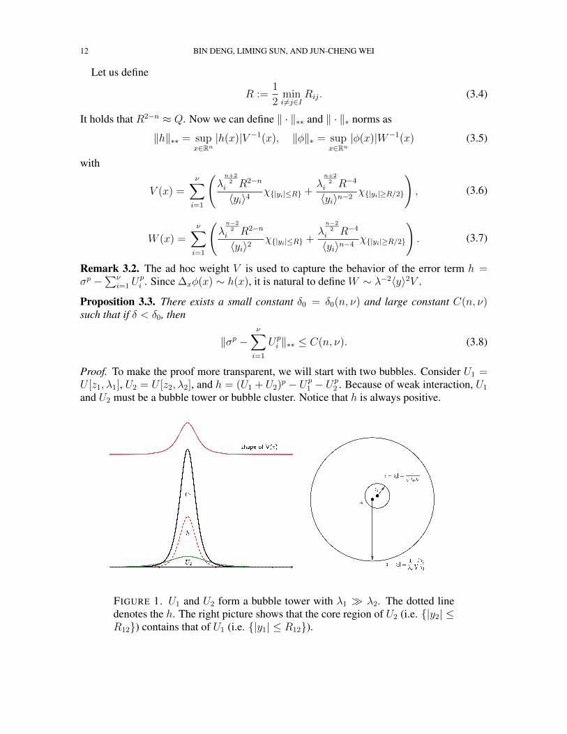
Proof. To make the proof more transparent, we will start with two bubbles. Consider U1 =U [z1, λ1], U2 = U [z2, λ2], and h = (U1 + U2)p − Up

1 − Up2 . Because of weak interaction, U1

and U2 must be a bubble tower or bubble cluster. Notice that h is always positive.

FIGURE 1. U1 and U2 form a bubble tower with λ1 λ2. The dotted linedenotes the h. The right picture shows that the core region of U2 (i.e. |y2| ≤R12) contains that of U1 (i.e. |y1| ≤ R12).


• Bubble tower (see Figure 1): Without loss of generality (WLOG), we can assume λ1 > λ2

and R12 =√λ1/λ2 = ε−1

12 1. In the rescaled z1-centered coordinate y1 = λ1(x− z1), wesee that U1(x) = λ

(n−2)/21 U(y1), where U(y) = U [0, 1](y), and

U2(x) =λ

(n−2)/21 R2−n

12

(1 + ε412|y1 − ξ2|2)(n−2)/2

, (3.9)

with |ξ2| = |λ1(z2 − z1)| ≤ R212. If |y1| ≤ R12/2, then U2 . U1,

h . Up−11 U2 ≈

λ(n+2)/21 R2−n

12

〈y1〉4. (3.10)

If R12/3 ≤ |y1| ≤ 2R212, then U1 ≈ λ

(n−2)/21 |y1|2−n and U2 ≈ λ

(n−2)/21 R2−n

12 . Settingy = y1/R12, then

h . λ(n+2)/21 R

−(n+2)12

∣∣∣∣(1 +1

|y|n−2

)p− 1− 1

|y|p(n−2)

∣∣∣∣.λ

(n+2)/21 R

−(n+2)12

|y|n−2≈ λ

(n+2)/21 R−4

12

〈y1〉n−2.

(3.11)

On the other hand, in the rescaling z2-centered coordinate y2 = λ2(x − z2), we see thatU2(x) = λ

(n−2)/22 U(y2) and

U1(x) =λ

(n−2)/22 R2−n

12

(ε412 + |y2 − ξ1|2)(n−2)/2

, (3.12)

where ξ1 = λ2(z1 − z2) with |ξ1| < 1. Keep in mind that y2 − ξ1 = ε212y1. Thus, if

1 ≤ |y2 − ξ1| ≤ R12/2, it means R212 ≤ |y1| ≤ R3

12/2. In this region, we have U1 . U2,

h . Up−12 U1 ≈

λ(n+2)/22 R2−n

12

〈y2〉4. (3.13)

In the outer region |y2 − ξ1| ≥ R12/3, it is easy to see that

h . Up2 ≈

λ(n+2)/22 R−2

12

〈y2〉n.λ

(n+2)/22 R−4

12

〈y2〉n−2. (3.14)

From (3.10), (3.11), (3.13) and (3.14), we conclude

h .2∑i=1

(λn+22

i R2−n12

〈yi〉4χ|yi|≤R12/2 +

λn+22

i R−412

〈yi〉n−2χ|yi|≥R12/3

)

≤2∑i=1

(λn+22

i R2−n

〈yi〉4χ|yi|≤R/2 +

λn+22

i R−4


),

(3.15)

for any 0 < R ≤ R12.


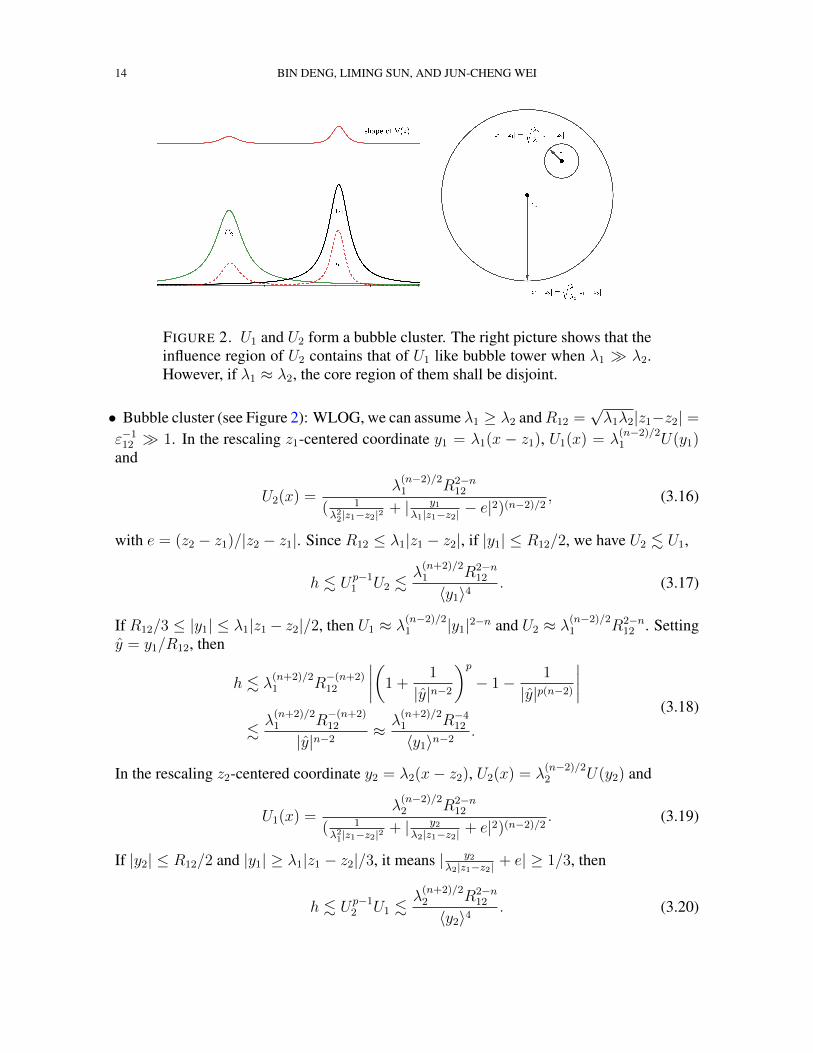
FIGURE 2. U1 and U2 form a bubble cluster. The right picture shows that theinfluence region of U2 contains that of U1 like bubble tower when λ1 λ2.However, if λ1 ≈ λ2, the core region of them shall be disjoint.

• Bubble cluster (see Figure 2): WLOG, we can assume λ1 ≥ λ2 andR12 =√λ1λ2|z1−z2| =

ε−112 1. In the rescaling z1-centered coordinate y1 = λ1(x − z1), U1(x) = λ

(n−2)/21 U(y1)

and

U2(x) =λ

(n−2)/21 R2−n

12

( 1λ22|z1−z2|2

+ | y1λ1|z1−z2| − e|

2)(n−2)/2, (3.16)

with e = (z2 − z1)/|z2 − z1|. Since R12 ≤ λ1|z1 − z2|, if |y1| ≤ R12/2, we have U2 . U1,

h . Up−11 U2 .

λ(n+2)/21 R2−n

12

〈y1〉4. (3.17)

If R12/3 ≤ |y1| ≤ λ1|z1− z2|/2, then U1 ≈ λ(n−2)/21 |y1|2−n and U2 ≈ λ

(n−2)/21 R2−n

12 . Settingy = y1/R12, then

h . λ(n+2)/21 R

−(n+2)12

∣∣∣∣(1 +1

|y|n−2

)p− 1− 1

|y|p(n−2)

∣∣∣∣.λ

(n+2)/21 R

−(n+2)12

|y|n−2≈ λ

(n+2)/21 R−4

12

〈y1〉n−2.

(3.18)

In the rescaling z2-centered coordinate y2 = λ2(x− z2), U2(x) = λ(n−2)/22 U(y2) and

U1(x) =λ

(n−2)/22 R2−n

12

( 1λ21|z1−z2|2

+ | y2λ2|z1−z2| + e|2)(n−2)/2

. (3.19)

If |y2| ≤ R12/2 and |y1| ≥ λ1|z1 − z2|/3, it means | y2λ2|z1−z2| + e| ≥ 1/3, then

h . Up−12 U1 .

λ(n+2)/22 R2−n

12

〈y2〉4. (3.20)


In the outer region |y2| ≥ R12/3 and |y1| ≥ λ1|z1 − z2|/3 ≥ R12/3, we have

h . Up1 + Up

2 .λ

(n+2)/21 R−4

12

〈y1〉n−2+λ

(n+2)/22 R−4

12

〈y2〉n−2. (3.21)

From (3.17), (3.18), (3.20) and (3.21), we also have (3.15).• For any finite number of bubbles, we shall use a simple inequality (see Lemma A.6)

h = σp −ν∑i=1

Upi ≤

∑i 6=j

[(Ui + Uj)p − Up

i − Upj ].

Each one on the RHS can be bounded by the above estimates of two bubbles, see (3.15).Summing them up, one can obtain h ≤ C(n, ν)V (x).

Remark 3.4. In order to have a simple form of V , we bound h just by 〈yi〉2−n in (3.14) and(3.21). In fact, h decays faster than V at infinity. Such relaxation causes a minor problemfor n = 6 when estimating

∫|yi|≥R,|yj |≥R VW in Proposition 3.9. Check the estimate (B.16)

and (B.20) in Lemma B.2. Thanks to the fact that if n = 6 then p = 2 and σp −∑ν

i=1 Upi =∑

i 6=j UiUj . We can get around this and directly estimate the integral∫UiUjρ0. Check the

estimate (B.37) in Lemma B.3.

Lemma 3.5. There exist a positive δ0 and a constant C, independent of δ, such that for allδ 6 δ0, if Ui1≤i≤ν is a δ-interacting bubble family and φ solves the equation

∆φ+ pσp−1φ = h,∫Up−1i φZa

i = 0, i = 1, · · · , ν; a = 1, · · · , n+ 1,(3.22)

then

‖φ‖∗ ≤ C‖h‖∗∗. (3.23)

Proof. We use blow-up arguments to prove (3.23). Suppose there are k →∞, 1k-interacting

bubble familiesU

(k)i := U [z

(k)i , λ

(k)i ]

1≤i≤ν, h = hk with ‖hk‖∗∗ → 0, and φ = φk with

‖φk‖∗ = 1 solving the equation∆φk + pσp−1

k φk = hk, in Rn,∫Up−1i Za

i φk = 0, i = 1, · · · , ν; 1 ≤ a ≤ n+ 1.(3.24)

For simplicity, here and after we denote Ui := U(k)i and σk :=

∑νi=1 U

(k)i .

At the beginning, let us introduce some notations. After finite steps of choosing subse-quences, we can make the following assumptions. For each i ∈ I = 1, · · · , ν, let z(k)

ij :=

λ(k)i (z

(k)j − z

(k)i ), j ∈ I \ i, we can assume that limk→∞ z

(k)ij exists or limk→∞ z

(k)ij = ∞.

Then we divide indices I \ i into two groups:

Ii,1 := j ∈ I \ i | limk→∞

z(k)ij exists and lim

k→∞|z(k)ij | <∞,

Ii,2 := j ∈ I \ i | limk→∞

z(k)ij =∞.

(3.25)


Furthermore, we divide all bubbles into four groups: ones are higher (lower) than Ui in towerrelationship, ones are much higher (otherwise) than Ui in cluster relationship.

T+i := j ∈ I \ i | λ(k)

j ≥ λ(k)j , R

(k)ij =

√λ

(k)j /λ

(k)i ,

T−i := j ∈ I \ i | λ(k)j < λ

(k)i , R

(k)ij =

√λ

(k)i /λ

(k)j ,

C+i := j ∈ I \ i | lim

k→∞λ

(k)j /λ

(k)i =∞, R(k)

ij =

√λ

(k)i λ

(k)j |z

(k)i − z

(k)j |,

C−i := j ∈ I \ i | limk→∞

λ(k)j /λ

(k)i <∞, R(k)

ij =

√λ

(k)i λ

(k)j |z

(k)i − z

(k)j |.

(3.26)

Recall that y(k)i = λ

(k)i (x− z(k)

i ). Let us define

Li := maxj∈Ii,1

limk→∞|z(k)ij |

+ L,

Ω(k) :=⋃i∈I

|y(k)i | ≤ Li,

Ω(k)i := |y(k)

i | ≤ Li⋂ ⋂

j∈T+i ∪C

+i

|y(k)i − z

(k)ij | ≥ ε

,

(3.27)

with a large constant L = L(n, ν) and a small constant ε = ε(n, ν) to be determined later.When k is large enough, our choice of Li will make sure |y(k)

i − z(k)ij | = ε ⊂ |y(k)

i | ≤ Lifor j ∈ (T+

i ∪ C+i ) ∩ Ii,1. See Figure 3 for an illustration of Ω

(k)i in a simple case.

For simplicity, here and after we drop the superscript if there is no confusion. It is conve-nient to denote W =

∑i∈I(wi,1 + wi,2) and V =

∑i∈I(vi,1 + vi,2) with

wi,1(x) =λn−22

i R2−n

〈yi〉2χ|yi|≤R, wi,2(x) =

λn−22

i R−4

〈yi〉n−4χ|yi|≥R/2,

vi,1(x) =λn+22

i R2−n

〈yi〉4χ|yi|≤R, vi,2(x) =

λn+22

i R−4

〈yi〉n−2χ|yi|≥R/2,

(3.28)

where R = R(k) = 12

mini 6=jR(k)ij → ∞ as k →∞.

Since ‖φk‖∗ = 1, we have |φk|(x) ≤ W (x) and there exists a sequence of points xkk∈Nsuch that

|φk|(xk) = W (xk). (3.29)

First, going to a subsequence if necessary, we consider the case that xkk∈N ⊂ Ω.Case 1: xkk∈N ⊂ Ωi0 for some i0 ∈ I . Let i0 = 1 and define

φk(y1) := W−1(xk)φk(x) with y1 = λ1(x− z1),

hk(y1) := λ−21 W−1(xk)hk(x), σk(y1) := σk(x).

(3.30)


Then φk satisfy∆φk(y1) + pλ−2

1 σp−1k (y1)φk(y1) = hk(y1) in Rn,∫

Up−1Zaφkdy1 = 0, 1 ≤ a ≤ n+ 1.(3.31)

Here U = U [0, 1](y1) and Za = Za(y1) = Za1 (x) defined in (3.1). Let zj = z

(k)1j , zj =

limk→∞ z(k)1j and

E1 :=⋂

j∈T+1 ∩I1,1

|y1 − zj| ≥ 1/M, E2 :=⋂

j∈C+1 ∩I1,1

|y1 − zj| ≥ |zj|/M.

Let

KM := |y1| ≤M ∩ E1 ∩ E2. (3.32)

Suppose M ≥ 2 maxL1, ε−1, it is easy to see that Ω

(k)1 ⊂⊂ KM for k large.

Claim 1. In each compact subset KM , it holds that, as k →∞,

λ−21 σp−1

k → U [0, 1], |hk| → 0, (3.33)

uniformly. Moreover, we have

|φk|(y1) . |y1 − zj|4−n + 1, j ∈ T+1 ∪ C+

1 . (3.34)

We postpone the proof of Claim 1 and finish the blow-up argument in Case 1. By thestandard elliptic regularity theorem, the Claim 1 shows that there exists a subsequence of φkuniformly converges in each KM . Furthermore, by the diagonal arguments, let M →∞, wehave a subsequence of φk weakly converges to φ with

∆φ+ pUp−1φ = 0, in Rn \ zj | j ∈ (T+1 ∪ C+

1 ) ∩ I1,1,|φ|(y1) . |y1 − zj|4−n + 1, j ∈ (T+

1 ∪ C+1 ) ∩ I1,1,∫

Up−1Zaφdy1 = 0, 1 ≤ a ≤ n+ 1.

(3.35)

Notice that all singular zj are removable. Together with the non-degeneracy of Talenti bub-bles, we get φ ≡ 0. However, since |Yk| ≤ L1, going to a subsequence if necessary, thenlimk→∞ Yk = Y∞ and consequently φ(Y∞) = 1. This is a contradiction.

Case 2: xkk∈N ⊂ Ω \ (∪i∈IΩi). There exist some i ∈ I such that, choosing a subse-quence if necessary, xkk∈N ⊂ Ai where

Ai :=⋃j∈Ji

|yi| ≤ Li, |yi − zij| ≤ ε, |yj| ≥ Lj , Ji = T+i ∪ C+

i . (3.36)

We can choose the smallest Ai0 such that, for each Ai ⊃ xkk∈N, it holds that λi0 ≥ λi.For simplicity, let i0 = 1 and take notations as before. See Figure 3 for Ai in a simple case.Denote J1 = T+

1 ∪ C+1 , let us define

W (x) :=∑j∈J1

(wj,1(x) + wj,2(x)) + w1,1(x),

V (x) :=∑j∈J1

(vj,1(x) + vj,2(x)) + v1,1(x).(3.37)


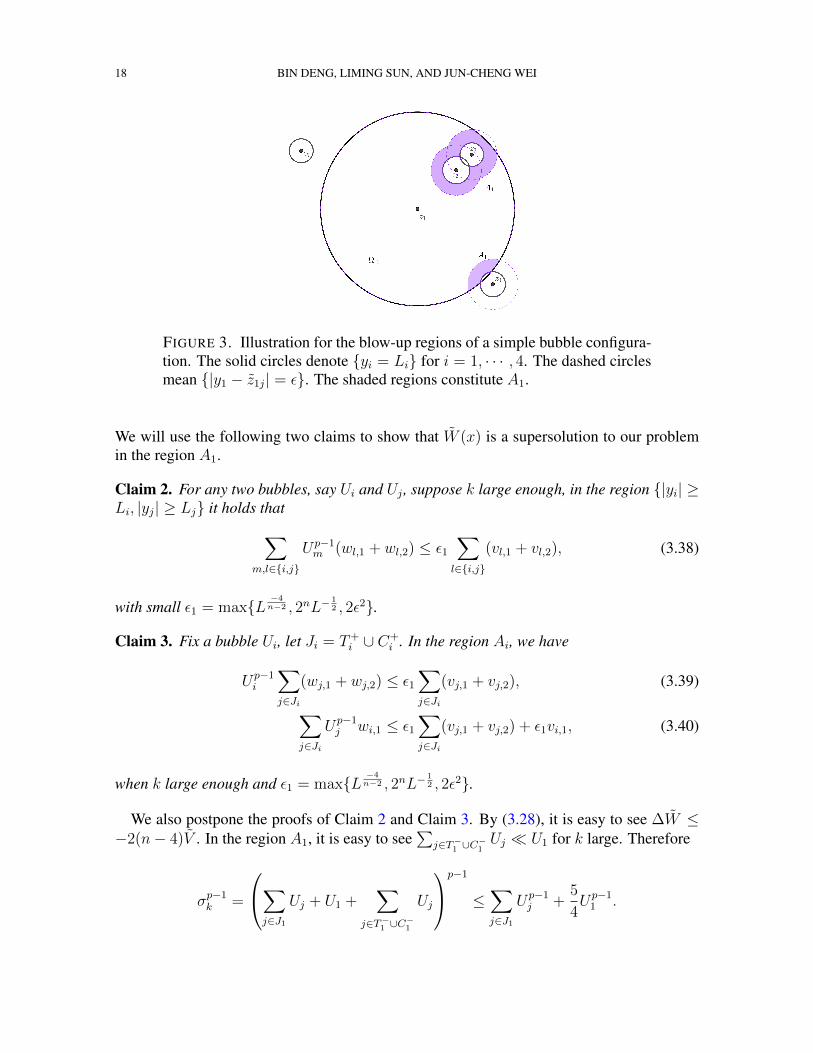
FIGURE 3. Illustration for the blow-up regions of a simple bubble configura-tion. The solid circles denote yi = Li for i = 1, · · · , 4. The dashed circlesmean |y1 − z1j| = ε. The shaded regions constitute A1.

We will use the following two claims to show that W (x) is a supersolution to our problemin the region A1.

Claim 2. For any two bubbles, say Ui and Uj , suppose k large enough, in the region |yi| ≥Li, |yj| ≥ Lj it holds that∑

m,l∈i,j

Up−1m (wl,1 + wl,2) ≤ ε1

∑l∈i,j

(vl,1 + vl,2), (3.38)

with small ε1 = maxL−4n−2 , 2nL−

12 , 2ε2.

Claim 3. Fix a bubble Ui, let Ji = T+i ∪ C+

i . In the region Ai, we have

Up−1i

∑j∈Ji

(wj,1 + wj,2) ≤ ε1∑j∈Ji

(vj,1 + vj,2), (3.39)

∑j∈Ji

Up−1j wi,1 ≤ ε1

∑j∈Ji

(vj,1 + vj,2) + ε1vi,1, (3.40)

when k large enough and ε1 = maxL−4n−2 , 2nL−

12 , 2ε2.

We also postpone the proofs of Claim 2 and Claim 3. By (3.28), it is easy to see ∆W ≤−2(n− 4)V . In the region A1, it is easy to see

∑j∈T−1 ∪C

−1Uj U1 for k large. Therefore

σp−1k =

∑j∈J1

Uj + U1 +∑

j∈T−1 ∪C−1

Uj

p−1

≤∑j∈J1

Up−1j +

5

4Up−1

1 .


Consequently, it follows from Claim 2 and Claim 3 that

σp−1k W ≤

∑i,j∈J1

Up−1i (wj,1 + wj,2) +

5

4Up−1

1

∑j∈J1

(wj,1 + wj,2)

+ w1,1

∑j∈J1

Up−1j +

5

4Up−1

1 w1,1

≤ (4ν2ε1 +5

4)V in A1.

(3.41)

Then, by choosing L large and ε small such that (4ν2ε1 + 5/4)p ≤ 3,

∆W + pσp−1k W ≤ −V in A1. (3.42)

From Case 1, we conclude that, for k large,

|φk|(x) ≤ C‖hk‖∗∗W (x) in ∪i∈I Ωi, (3.43)

with a constant C = C(n, ν). On the other hand, if i ∈ T−1 , then |yi| = λiλ1|y1 − zi| ≤ Li.

We have, for k large,

w1,1

wi,1=

(λ1

λi

)n−22 〈yi〉2

〈y1〉2≥ L−2

(λ1

λi

)n−22

1,

v1,1

vi,1=

(λ1

λi

)n+22 〈yi〉4

〈y1〉4≥ L−4

(λ1

λi

)n+22

1.

(3.44)

If i ∈ C−1 , then |yi| = λiλ1|y1 − zi| ≥ λi|zi|

2λ1= λi|z1−zi|

2. We have

w1,1

wi,2= R6−n

(λ1

λi

)n−22 〈yi〉n−4

〈y1〉2≥ 24−nL−2R2

(λ1

λi

) 1,

v1,1

vi,2= R6−n

(λ1

λi

)n+22 〈yi〉n−2

〈y1〉4≥ 22−nL−4R4

(λ1

λi

)2

1.

(3.45)

From (3.44) and (3.45), we have

W = W +∑

j∈T−1 ∪C−1

(wj,1 + wj,2) ≤ 2W in A1,

V = V +∑

j∈T−1 ∪C−1

(vj,1 + vj,2) ≤ 2V in A1.(3.46)

By the definition (3.27), it is easy to see that ∂A1 ⊂ ∪i∈I∂Ωi for k large. From (3.43) and(3.46), we have

|φk|(x) ≤ 10C‖hk‖∗∗W (x) on ∂A1 ⊂ ∪i∈I∂Ωi. (3.47)

Together with (3.41), it holds that±10C‖hk‖∗∗W is an upper (lower) barrier for φk in A1. Itfollows that

|φk|(xk)W−1(xk) ≤ 10C‖hk‖∗∗ → 0. (3.48)

It contradicts to (3.29) since W (xk) ≥ W (xk).


Case 3: xkk∈N ⊂ Ωc = ∪i∈I|yi| > Li. As before, it is easy to see that ∆W ≤−2(n− 4)V . From Claim 2, we also have

σp−1k W ≤ ν2ε1V in Ωc. (3.49)

Then,

∆W + pσp−1k W ≤ −V in Ωc. (3.50)

From Case 1 and Case 2, we conclude that, for k large,

|φk|(x) ≤ C‖hk‖∗∗W (x) in Ω. (3.51)

In particular, we have

|φk|(x) ≤ C‖hk‖∗∗W (x) on ∂Ωc = ∂Ω. (3.52)

Thus ±C‖hk‖∗∗W is an upper (lower) barrier for φk in Ωc. It follows that

|φk|(xk)W−1(xk) ≤ C‖hk‖∗∗ → 0. (3.53)

It contradicts to (3.29).To complete the proof of (3.23), it suffices to prove the three claims above.

Proof of Claim 1. To prove the claim, we need to use a simple inequality∑i ai∑i bi≤ max

iaibi, (3.54)

holds for any positive numbers ai, bi. Thus by (3.31)

|φk|(y1) =|φk(x)|W (xk)

≤ W (x)

Wk(x)≤ max

j

wj,1(x) + wj,2(x)

wj,1(xk) + wj,2(xk)

,

|hk|(x) =|hk(x)|λ2

1W (xk)≤ ‖hk‖∗∗V (x)

λ21W (xk)

≤ ‖hk‖∗∗maxj

vj,1(x) + vj,2(x)

λ21wj,1(xk) + λ2

1wj,2(xk)

.

We shall estimate the RHS of the above two equations on each compact subset KM . Theyare divided into the following four cases.The case j ∈ T+

1 . By (3.12), we have

Uj(x) ≈λn−22

j

〈yj〉n−2≈

λn−22

1 R2−n1j

(ε21j + |y1 − zj|)n−2

.Mn−2λn−22

1 R2−n1j . (3.55)

Let Yk = λ1(xk − z1). Since |yj| = R21j|y1 − zj| ≥ R2

1j/M ≥ R for k large, we only needto consider

wj,2(x)

wj,2(xk)≈

(ε21j + |Yk − zj|)n−4

(ε21j + |y1 − zj|)n−4

.1

|y1 − zj|n−4, (3.56)

vj,2(x)

λ21wj,2(xk)

≈(ε2

1j + |Yk − zj|)n−4

(ε21j + |y1 − zj|)n−2

.Mn−2. (3.57)

The case j ∈ T−1 . By (3.9), we have

Uj(x) ≈λn−22

1 R2−n1j

(1 + ε21j|y1 − zj|)n−2

. λn−22

1 R2−n1j . (3.58)


It holds that |yj| = R−21j |y1 − zj| ≤MR−2

1j ≤ R for k large. Then we have

wj,1(x)

wj,1(xk)≈

(1 + ε21j|Yk − zj|)2

(1 + ε21j|y1 − zj|)2

. 1, (3.59)

vj,1(x)

λ21wj,1(xk)

≈ R−41j

(1 + ε21j|Yk − zj|)2

(1 + ε21j|y1 − zj|)4

. R−41j . (3.60)

The case j ∈ C+1 . Let λ = λj/λ1, then R1j =

√λ|zj| and |zj| ≥ 1. It holds that, no matter

|zj| <∞ or |zj| =∞, we have |yj| = λ|y1 − zj| ≥√λR1j/M ≥ R for k large. Then

Uj(x) ≈ λn−22

1

(λ−1/2 + λ1/2|y1 − zj|)n−2. λ

n−22

1 Mn−2R2−n1j . (3.61)

Then we havewj,2(x)

wj,2(xk)≈ (λ−1/2 + λ1/2|Yk − zj|2)n−4

(λ−1/2 + λ1/2|y1 − zj|)n−4.

1

|y1 − zj|n−4, (3.62)

vj,2(x)

λ21wj,2(xk)

≈ λR−21j

(λ−1/2 + λ1/2|Yk − zj|)n−4

(λ−1/2 + λ1/2|y1 − zj|)n−2. Mn−2R−2

1j |zj|−2 ≤Mn−2R−21j . (3.63)

The case j ∈ C−1 . Let λ = λj/λ1, then R1j =√λ|zj| ≤ (1 + θj)|zj| with θj =

limk→∞ λ(k)j /λ

(k)1 . It holds that |y1| ≤M ≤ |zj|/2 for k large. Then |y1 − zj| ≥ |zj|/2,

Uj(x) ≈ λn−22

1

(λ−1/2 + λ1/2|y1 − zj|)n−2. λ

n−22

1 R2−n1j . (3.64)

Furthermore, we havewj,2(x)

wj,2(xk)≈ (λ−1/2 + λ1/2|Yk − zj|2)n−4

(λ−1/2 + λ1/2|y1 − zj|)n−4. R4−n

1j , (3.65)

vj,2(x)

λ21wj,2(xk)

≈ λR−21j

(λ−1/2 + λ1/2|Yk − zj|)n−4

(λ−1/2 + λ1/2|y1 − zj|)n−2. R−n1j . (3.66)

It is easy to see that

U1(x) = U(y1),w1,1(x)

w1,1(xk)≈ 〈Yk〉

2

〈y1〉2. 1,

v1,1(x)

λ21w1,1(xk)

≈ 〈Yk〉2

〈y1〉4. 1. (3.67)

From (3.55), (3.58), (3.61), (3.64) and (3.67), we get

λ−21 σp−1

k (y1) = U [0, 1](y1) + o(1)→ U [0, 1](y1). (3.68)

From (3.55), (3.58), (3.61), (3.64) and (3.67), we get

|hk| ≤ ‖hk‖∗∗V (x)

λ21W (xk)

.Mn−2‖hk‖∗∗ → 0. (3.69)

From (3.56), (3.59), (3.62), (3.65) and (3.67), we see that the singularities only happen forj ∈ (T+

1 ∪ C+1 ) ∩ I1,1 with

|φk|(y1) . W (x)W (xk)−1 . max

j|y1 − zj|4−n+ 1. (3.70)


Proof of the Claim 2. Here and after, we always assume k is large enough. WLOG, weassume i = 1 and j = 2. It is easy to see the claim holds when m = l,

2∑l=1

Up−1i (wl,1 + wl,2) ≤ ε1

2∑l=1

(vl,1 + vl,2). (3.71)

It reduces to consider the case m 6= l. We divide it to the following two main cases.(1) The case λ1 ≥ λ2 and R12 =

√λ1/λ2. Let ξ1 = λ2(z1 − z2) and ξ2 = λ1(z2 − z1). It

holds that |ξ1| ≤ 1 and |ξ2| ≤ R212. Since y1 = R2

12(y2 − ξ1), then 〈y1〉 ≥ 12R2

12〈y2〉 on theset |y1| ≥ L1, |y2| ≥ L2. We have

Up−11 (w2,1 + w2,2) =

λ21

〈y1〉4(w2,1 + w2,2) ≤ 16λ2

2〈y2〉−4(w2,1 + w2,2)

≤ 16〈y2〉−2(v2,1 + v2,2) ≤ ε1(v2,1 + v2,2).

(3.72)

Observe that |y1 − ξ2| = R212|y2| ≥ L2R

212, then |y1| ≥ (L2 − 1)R2

12. In the region |y1| ≥L1, |y2| ≥ L2, we get

Up−12 (w1,1 + w1,2) =

λ22

〈y2〉4λn−22

1 R−4

〈y1〉n−4χ|y1|≥(L2−1)R2

12.(3.73)

First, we bound the above term on the set L2 ≤ |y2| ≤ L2R12, |y1| ≥ (L2 − 1)R212, that is

λ22

〈y2〉4λn−22

1 R−4

〈y1〉n−4=λn+22

2 R−4

〈y2〉4Rn−2

12

〈y1〉n−4≤ (L2 − 1)4−nλ

n+22

2 R−4

〈y2〉41

Rn−612

≤ Ln−62

(L2 − 1)n−4

(λn+22

2 R2−n

〈y2〉4χ|y2|≤R +

λn+22

2 R−4

〈y2〉n−2χR≤|y2|≤L2R12

)≤ ε1(v2,1 + v2,2).

(3.74)

Second, on |y2| ≥ L2R12, |y1| ≥ (L2−1)R212, we have 〈y1〉 = 〈R2

12(y2−ξ1)〉 ≥ 12R2

12〈y2〉,

λ22

〈y2〉4λn−22

1 R−4

〈y1〉n−4=λn+22

2 R−4

〈y2〉4Rn−2

12

〈y1〉n−4≤ v2,2

〈y2〉n−6Rn−212

〈y1〉n−4≤ ε1v2,2. (3.75)

(2) The case λ1 ≥ λ2 and R12 =√λ1λ2|z1 − z2|. Notice that |ξ2| =

√λ1/λ2R12 and

y2 = λ2λ−11 (y1 − ξ2). Then on the set L1 ≤ |y1| ≤ 1

2

√λ1/λ2R12, we have 〈y2〉 ≥

12

√λ2/λ1R12. Consequently

Up−12 w1,1 =

λ22

〈y2〉4λn−22

1 R2−n

〈y1〉2χL1≤|y1|≤R ≤ 16λ2

1R−412

λn−22

1 R2−n

〈y1〉2≤ ε1v1,1. (3.76)

Next consider Up−12 w1,2. To bound it, we divide it into two cases. First, suppose λ2|z1−z2| ≥

(L2)14 , then on the set R < |y1| < 1

2

√λ1/λ2R12

Up−12 w1,2 ≤ 16λ2

1R−412

λn−22

1 R−4

〈y1〉n−4= 16v1,2

〈y1〉2

R412

<16

λ22|z1 − z2|2

v1,2 ≤16√L2

v1,2. (3.77)


On the set |y1| > 12

√λ1/λ2R12, then

Up−12 w1,2 =

λ22

〈y2〉4λn−22

1 R−4

〈y1〉n−4= v2,1

(λ1/λ2)n−22 Rn−6

〈y1〉n−4<

2n−4

λ22|z1 − z2|2

v2,1 <2n−4

√L2

v2,1.

Second, suppose |ξ1| = λ2|z1 − z2| ≤ L1/42 . On the set L2 ≤ |y2| ≤ R, since y1 =

λ1λ2

(y2 − ξ1), then |y1| ≥ λ1λ2

L2

2≥√L2

2R2

12 and

Up−12 w1,2 =

λ22

〈y2〉4λn−22

1 R−4

〈y1〉n−4≤ v2,1

(λ1/λ2)n−22 Rn−6

(12

√L2R2

12)n−4≤ (

1

2

√L2)4−nv2,1 ≤ ε1v2,1.

On the set |y2| ≥ R,

Up−12 w1,2 = v2,2

(λ1λ2

)n−22 〈y2〉n−6

〈y1〉n−4≤ v2,2

(λ1λ2

)n−22 〈y2〉n−6

〈12λ1λ2y2〉n−4

≤ v2,2

2n−4(λ1λ2

)6−n2

〈y2〉2≤ ε1v2,2.

Let us consider the term Up−11 w2,1. On the set L2 < |y2| < R, |y1| < R, one has

〈y2〉 ≥ 12

√λ2/λ1R12 and

Up−11 w2,1 =

λ21

〈y1〉4λn−22

2 R2−n

〈y2〉2≤ λ2

1

〈y1〉4λn−22

2 R2−n

(12

√λ2/λ1R12)2

= 4(λ2

λ1

)n−42 R−2

12 v1,1 ≤ εv1,1.

On the set L2 < |y2| < R,R < |y1| ∩ L2(λ2/λ1)2v1,2 ≥ v2,1, one has

Up−11 w2,1 =

λ21

〈y1〉4λn−22

2 R2−n

〈y2〉2= v2,1

〈y2〉2

〈y1〉4(λ1

λ2

)2 ≤ L2〈y2〉2

〈y1〉4v1,2 ≤ L2R

−2v1,2. (3.78)

On the set L2 < |y2| < R,R < |y1| ∩ L2(λ2/λ1)2v1,2 ≤ v2,1, one has 〈y1〉n−2 ≥L2(λ1/λ2)

n−22 Rn−6〈y2〉4, then

Up−11 w2,1 = v2,1

〈y2〉2

〈y1〉4

(λ1

λ2

)2

≤ v2,1L− 4n−2

2 R−4(n−6)n−2 〈y2〉

2n−20n−2 ≤ ε1v2,1, (3.79)

here we have use L2 ≤ |y2| ≤ R.It remains to consider the term Up−1

1 w2,2. First, on the set |y2| ≥ R, |y1| ≤ R, similarto (3.76), one has

Up−11 w2,2 =

λ21

〈y1〉4λn−22

2 R−4

〈y2〉n−4≤ λ2

1

〈y1〉4λn−22

2 R2−n

〈y2〉2≤ ε1v1,1. (3.80)

Second, on the set |y2| ≥ R, |y1| ≥ R ∩ v1,2 ≥ v2,2, one has 〈y1〉/〈y2〉 ≤ (λ1λ2

)n+2

2(n−2) ,

Up−11 w2,2 =

λ21

〈y1〉4λn−22

2 R−4

〈y2〉n−4≤ v1,2

〈y1〉n−6

〈y2〉n−4

(λ2

λ1

)n−22

≤ v1,21

〈y2〉2

(λ2

λ1

) 8n−2

≤ ε1v1,2.

On the set |y2| ≥ R, |y1| ≥ R ∩ v1,2 ≤ v2,2, one has 〈y1〉 ≥ 〈y2〉(λ1/λ2)n+2

2(n−2)

Up−11 w2,2 =

λ21

〈y1〉4λn−22

2 R−4

〈y2〉n−4= v2,2

(λ1

λ2

)2 〈y2〉2

〈y1〉4≤ v2,2

(λ2/λ1)8

n−2

〈y2〉2≤ ε1v2,2.


Proof of the Claim 3. WLOG we assume i = 1. By the definition (3.26), we have λj λ1.Let λ = λj/λ1, ξ1 = λj(z1 − zj) and ξj = zj = λ1(zj − z1). Observe that, if j ∈ C+

1 ,|yj| ≤ R

√λR1j = |ξ1|, then |yj − ξ1| ≥ |ξ1|/2. Thus, on the set Lj ≤ |yj| ≤ R, no

matter j ∈ C+1 or T+

1 ,

λ〈y1〉2 = λ+ λ−1|yj − ξ1|2 ≥1

2R2

1j, j ∈ T+1 ∪ C+

1 . (3.81)

It follows from (3.81) that, on the set Lj ≤ |yj| ≤ R,

Up−11 wj,1 =

λ21

〈y1〉4λn−22

j R2−n

〈yj〉2≤ 16R−4

1j

λn+22

j R2−n

〈yj〉2≤ ε1vj,1. (3.82)

Moreover, on the set |yj| ≥ R, |y1− ξj| ≤ ε, it holds that 〈yj〉2 = 1+λ2|y1− ξj|2 ≤ 2λ2ε2

and

Up−11 wj,2 =

λ21

〈y1〉4λn−22

j R−4

〈yj〉n−4=〈yj〉2

λ2〈y1〉4vj,2 ≤ 2ε2vj,2 ≤ ε1vj,2. (3.83)

Together with (3.82) and (3.83), we prove the (3.39).If Lj ≤ |yj| ≤ R, it is easy to see that

Up−1j w1,1 =

λ2j

〈yj〉4λn−22

1 R2−n

〈y1〉2=

λ2−n2

〈y1〉2vj,1 ≤ ε1vj,1. (3.84)

For |yj| > R, one can use the same type of estimates (3.78) and (3.79) to prove

Up−1j w1,1 ≤ ε1(vj,2 + v1,1).

Combining the above claims, we complete the proof.

Next, we estimate the coefficients cjb in (3.2).

Lemma 3.6. Suppose σ is the sum of a family of δ-interacting bubbles. If φ, h and cjb satisfy(3.2), then

|cjb| . Q‖h‖∗∗ +Qp‖φ‖∗, 1 ≤ j ≤ ν, 1 ≤ b ≤ n+ 1.

Proof. We shall multiply (3.2) by Zbj . By the Lemma A.5, for a, b ≤ n+ 1, there exist some

constants γb such that∑i,a

∫ciaU

p−1i Za

i Zbj = cjbγ

b +∑i 6=j

n+1∑a=1

ciaO(qij).

Fix 1 ≤ j ≤ ν, 1 ≤ b ≤ n+ 1. By the orthogonal condition in (3.2) and |Zbj | . Uj∣∣∣∣∫ pσp−1φZb

j

∣∣∣∣ =

∣∣∣∣∫ p(σp−1 − Up−1

j

)Zbjφ

∣∣∣∣. ‖φ‖∗

∫ (σp−1 − Up−1

j

)UjW.

(3.85)


Now we use the fact that, (σp−1 − Up−1i )Ui ≥ 0 for each i,

(σp−1 − Up−1j )Uj ≤

∑i

(σp−1 − Up−1i )Ui = σp −

∑i

Upi .

Then by Proposition 3.3, (3.85) can be bounded by∣∣∣∣∫ pσp−1φZbj

∣∣∣∣ . ‖φ‖∗ ∫ (σp −ν∑i=1

Upi )W . ‖φ‖∗

∫V (x)W (x)dx . Qp‖φ‖∗.

Here we have used Lemma B.2 in the last inequality (see similar estimates (3.107) and(3.109)). Similarly, by Lemma B.4 we have∣∣∣∣∫ hZb

j

∣∣∣∣ . ‖h‖∗∗ ν∑i=1

∫V Ujdx . Q‖h‖∗∗. (3.86)

Multiplying (3.2) by Zbj and integrating, we see that cjb satisfy the linear system

cjbγb +∑i 6=j

n+1∑a=1

ciaO(qij) =

∫pσp−1φZb

j +

∫hZb

j , 1 ≤ j ≤ ν, 1 ≤ b ≤ n+ 1.

Since qij ≤ Q ≤ δ the system is solvable and we prove the claim.

From Lemma 3.5 and 3.6, using the same argument as in the proof of Proposition 4.1 in[15], we can prove the following result:

Proposition 3.7. There exists positive δ0 and a constant C > 0, independent of δ, such thatfor all δ 6 δ0 and all h with ‖h‖∗∗ < ∞, problem (3.2) has a unique solution φ ≡ Lδ(h).Besides,

‖Lδ(h)‖∗ 6 C‖h‖∗∗,∣∣cia∣∣ 6 Cδ‖h‖∗∗.

Proposition 3.8. Suppose that δ is small enough. There exists a solution ρ0 and a family ofscalars (cia) which solve

∆φ+ [(σ + φ)p − σp] + σp −ν∑i=1

Upi =

∑i,a

ciaUpi Z

ai (3.87)

with|ρ0|(x) ≤ CW (x). (3.88)

Proof. Let

N1(φ) = (σ + φ)p − σp − pσp−1φ, (3.89)

N2 = σp −ν∑i=1

Upi . (3.90)

Then, (3.87) is equivalent to

φ = A(φ) =: −Lδ(N1(φ))− Lδ(N2), (3.91)

where Lδ is defined in Proposition 3.7. We will show that A is a contraction mapping.


First, it follows from Proposition 3.3 that there exists C2 = C2(n, ν)

‖N2‖∗∗ ≤ C2. (3.92)

Next, we claim that ‖N1(φ)‖∗∗ ≤ C1R−4(p−1)‖φ‖∗. In fact, since |N1(φ)| ≤ C|φ|p ≤

C‖φ‖p∗W p, then

‖N1(φ)‖∗∗ ≤ C‖φ‖∗ supRn

W p(x)V −1(x). (3.93)

Notice, for the first type weight function, say |yi| ≤ R, we have(λn−22

i R2−n

〈yi〉2

)p(〈yi〉4

λn+22

i R2−n

)= R−4〈yi〉4−2p ≤ R−4. (3.94)

For the second type weight, say R/2 ≤ |yi|, we have(λn−22

i R−4

〈yi〉n−4

)p(〈yi〉n−2

λn+22

i R−4

)= R−4(p−1)〈yi〉n−2−p(n−4) ≤ R−4(p−1), (3.95)

since n− 2− p(n− 4) ≤ 0. By the inequality (3.54), we get

W pV −1 ≤ R−4(p−1). (3.96)

Thus, there exists C1 = C1(n, ν) such that

‖N1(φ)‖∗∗ ≤ C1R−4(p−1)‖φ‖∗. (3.97)

Making C1 possibly larger so that we also have ‖Lδ(h)‖∗ ≤ C1‖h‖∗∗ in Proposition 3.7.Now define the space

E = u : u ∈ C(Rn) ∩D1,2(Rn), ‖u‖∗ ≤ C1C2 + 1. (3.98)

We claim that A is a contraction mapping from E to E. In fact, choosing δ small, then Rlarge such that R−4(p−1)C2

1(C1C2 + 1) ≤ 1, we have

‖A(φ)‖∗ ≤ C1‖N1(φ)‖∗∗ + C1‖N2‖∗∗≤ R−4(p−1)C2

1(C1C2 + 1) + C1C2 ≤ C1C2 + 1.(3.99)

Thus, A(E) ⊂ E. Furthermore,

‖A(φ1)− A(φ2)‖∗ ≤ ‖Lδ(N1(φ1))− Lδ(N1(φ2))‖∗∗≤ C1‖N1(φ1)−N1(φ2)‖∗∗.

(3.100)

If n ≥ 6, then N ′1(t) ≤ C|t|p−1. As a result,

|N1(φ1)−N1(φ2)| ≤ C(|φ1|p−1 + |φ2|p−1

)|φ1 − φ2|

≤ C(‖φ1‖p−1

∗ + ‖φ2‖p−1∗)‖φ1 − φ2‖∗W p.

(3.101)

Since W pV −1 ≤ R−4(p−1) 1 if δ small, we get

‖A(φ1)− A(φ2)‖∗ ≤1

2‖φ1 − φ2‖∗. (3.102)

Thus, A is a contraction. It follows from the contraction mapping theorem that there is aunique φ ∈ E, such that φ = A(φ). Moreover, it follows Proposition 3.7 that ‖φ‖∗ ≤ C.


3.2. Some estimates of the error. In this subsection, we will establish L2 estimates for the∇ρ, based on the point-wise estimates from the previous subsection.

Proposition 3.9. Suppose δ is small enough. We have the gradient estimates

‖∇ρ0‖L2 .

Q| logQ| 12 , if n = 6,

Qp2 , if n ≥ 7.

(3.103)

Proof. Multiplying ρ0 to (3.87) to get∫|∇ρ0|2 .

∫σp−1ρ2

0 +

∫|ρ0|p+1 +

∫(σp −

∑Upi )ρ0. (3.104)

It follows from Proposition 3.8 that |ρ0(x)| . W (x). By the Lemma B.1, we have∫σp−1ρ2

0 .ν∑i=1

∫Up−1i ρ2

0

.ν∑i=1

(∫|yi|≤R

λ2i

〈yi〉4λn−2i R4−2n

〈yi〉4dx+

∫|yi|≥R/2

λ2i

〈yi〉4λn−2i R−8

〈yi〉2n−8dx

)+∑i 6=j

(∫|yi|≤R

λ2j

〈yj〉4λn−2i R4−2n

〈yi〉4dx+

∫|yi|≥R/2

λ2j

〈yj〉4λn−2i R−8

〈yi〉2n−8dx

). R−n−2 ≈ Qp.

(3.105)

By Sobolev inequality, we have ∫|ρ0|p+1 . ‖∇ρ0‖p+1

L2 . (3.106)

Now consider the last term in (3.104). Proposition 3.3 says that |σp −∑

i Upi | . V (x).

• If n ≥ 7, using (3.6) and (3.7), we obtain∣∣∣∣∫ (σp −∑

Upi )ρ0

∣∣∣∣ . ∫ V (x)W (x)

≤ν∑

i,j=1

∫|yi|≤R|yj |≤R

λn+22

i R2−n

〈yi〉4λn−22

j R2−n

〈yj〉2+

∫|yi|≤R|yj |≥R/2

λn+22

i R2−n

〈yi〉4λn−22

j R−4

〈yj〉n−4

+ν∑

i,j=1

∫|yi|≥R/2|yj |≤R

λn+22

i R−4

〈yi〉n−2

λn−22

j R2−n

〈yj〉2+

∫|yi|≥R/2|yj |≥R/2

λn+22

i R−4

〈yi〉n−2

λn−22

j R−4

〈yj〉n−4.

(3.107)

By some tedious computations, Lemma B.2 shows∫(σp −

∑Upi )ρ0 . R−n−2 ≈ Qp. (3.108)

• If n = 6, then p = 2. By Lemma B.3, we have∣∣∣∣∫ (σ2 −∑

U2i )ρ0

∣∣∣∣ ≤∑i 6=j

∣∣∣∣∫ UiUjρ0

∣∣∣∣ . R−8 logR ≈ Q2| logQ|. (3.109)

Plugging (3.105), (3.106), (3.108), (3.109) into (3.104), we get (3.103).


Now consider ρ1 = ρ− ρ0. Recall ρ satisfies (2.3) and ρ0 satisfies (3.87). Thus ρ1 solves∆ρ1 + [(σ + ρ0 + ρ1)p − (σ + ρ0)p] +

∑i,a c

jaU

p−1j Za

j + f = 0.∫∇ρ1 · ∇Za

i = 0 i = 1, · · · , ν; a = 1, · · · , n+ 1.(3.110)

Now we decompose

ρ1 =ν∑i=1

βiUi +ν∑i=1

n+1∑a=1

βiaZai + ρ2, (3.111)

such that for all i = 1, · · · , ν and a = 1, · · · , n+ 1∫∇ρ2 · ∇Ui = 0 =

∫∇ρ2 · ∇Za

i . (3.112)

Lemma 3.10. If δ is small enough, then ρ2 satisfies

‖∇ρ2‖L2 .ν∑i=1

|βi|+ν∑i=1

n+1∑a=1

|βia|+ ‖f‖H−1 . (3.113)

Proof. Multiply the (3.110) by ρ2 and integrating, we get∫|∇ρ2|2 =

∫[(σ + ρ0 + ρ1)p − (σ + ρ0)p]ρ2 +

∫|ρ2f |

Since the elementary inequality

|(σ + ρ0 + ρ1)p − (σ + ρ0)p − p(σ + ρ0)p−1ρ1| . |ρ1|p (3.114)

then ∫|∇ρ2|2 ≤ p

∫|σ + ρ0|p−1|ρ1ρ2|+

∫|ρ1|p|ρ2|+

∫|ρ2f |. (3.115)

Notice the decomposition of ρ1 in (3.111),

p

∫|σ + ρ0|p−1|ρ1ρ2| ≤ p

∫|σ + ρ0|p−1ρ2

2 + B∫|σ + ρ0|p−1Ui|ρ2|

where B =∑

i |βi|+∑

i,a |βia|. By Holder inequality∫|σ + ρ0|p−1Ui|ρ2| . ‖ρ2‖L2∗‖|σ + ρ0|p−1Ui‖L(2∗)′ . ‖∇ρ2‖L2 ,∫|ρ1|p|ρ2| ≤ ‖ρ1‖pL2∗‖ρ2‖L2∗ . (B + ‖∇ρ2‖L2)p‖∇ρ2‖L2 .

(3.116)

It follows from the second variation estimate (for instance, see [4, Prop 3.1] and [20, Prop3.10]) and the orthogonal condition of ρ2 that there exists constant c < 1 such that

p

∫σp−1ρ2

2 ≤ c

∫|∇ρ2|2. (3.117)

Recall a simple inequality that if x > 0 and p ∈ (1, 2] then ‖x+ y|p−1 − |x|p−1| ≤ C|y|p−1

for any y. Consequently

p

∫|σ + ρ0|p−1ρ2

2 ≤ c

∫|∇ρ2|2 + C

∫|ρ0|p−1ρ2

2 ≤ (c+ C‖∇ρ0‖p−1L2 )‖∇ρ2‖2

L2 .


Therefore,

p

∫|σ + ρ0|p−1|ρ1ρ2| ≤ (c+ C‖∇ρ0‖p−1

L2 )‖∇ρ2‖2L2 + CB‖∇ρ2‖L2 . (3.118)

By Proposition 3.9, we can make ‖∇ρ0‖L2 1. Plugging in (3.116) and (3.118) to (3.115),

‖∇ρ2‖2L2 . B‖∇ρ2‖L2 + (B + ‖∇ρ2‖L2)p‖∇ρ2‖L2 + ‖f‖H−1‖∇ρ2‖L2 .

Choosing δ small such that ‖∇ρ2‖L2 < 1 and B < 1, then

‖∇ρ2‖L2 . B + ‖f‖H−1 . (3.119)

Lemma 3.11. If δ is small, then

|βi|+ |βia| . Q2 + ‖f‖H−1 .

Proof. We shall multiply (3.110) by Uk and integrate it. Before that, let us make somepreparations. It follows from (3.114) and |(σ + ρ0)p−1 − Up−1

k | .∑

i 6=k Up−1i + |ρ0|p−1 that∣∣∣∣∫ [(σ + ρ0 + ρ1)p − (σ + ρ0)p]Uk − p

∫Upkρ1

∣∣∣∣.∑i 6=k

∫Up−1i Uk|ρ1|+

∫|ρ1|pUk +

∫|ρ0|p−1ρ1Uk.

(3.120)

By Holder inequality and Sobolev inequality,∫|ρ1|pUk . Bp +

∫ρp2Uk . Bp + ‖f‖pH−1 ,∫

|ρ0|p−1ρ1Uk . ‖∇ρ0‖p−1L2 ‖∇ρ1‖L2‖Uk‖L2∗ . o(1) (B + ‖f‖H−1) ,∫

Up−1i |ρ1|Uk ≤ ‖ρ1‖L2∗‖Up−1

i Uk‖L(2∗)′ . o(1) (B + ‖f‖H−1) , i 6= k.

Here o(1) denotes a quantity goes to 0 when δ → 0. Multiplying (3.110) by Uk and integrateit. The above estimates give

−∫∇ρ1∇Uk + p

∫Upkρ1 .o(1) (B + ‖f‖H−1) +

∑j,a

|cja|∣∣∣∣∫ Up−1

j Zaj Uk

∣∣∣∣+

∫|fUk|.

We know that∫Up−1j Za

j Uk = 0 if j = k and∫Up−1j Za

j Uk .∫Upi Uk ≈ Q if j 6= k by

Lemma A.3. It follows from Proposition 3.3, Lemma 3.6 that |cja| . Q. Inserting theseestimates to the above equation,

(p− 1)

(∑i

βi∫Upi Uk +

∑i,a

βia

∫UpkZ

ai

). o(1)B +Q2 + ‖f‖H−1 ,

that is

(p− 1)βk +∑i 6=k

βiO(qik) +∑i,a

βiaO(qik) . o(1)B +Q2 + ‖f‖H−1 . (3.121)


Since∫∇ρ1 · ∇Zk

b = 0, then (3.111) and (3.112) imply

ν∑i=1

βi∫∇Ui · ∇Zb

k +ν∑i=1

n+1∑a=1

βia

∫∇Za

i · ∇Zbk = 0.

Using Lemma A.5, it is equivalent to∑i 6=k

βiO(qik) + βkb +∑

i 6=k,a6=b

βiaO(qik) = 0. (3.122)

Combining (3.121) and (3.122), we can get the conclusion.

Proposition 3.12. Suppose δ is small enough. We have

‖∇ρ1‖L2 . Q2 + ‖f‖H−1 .

Proof. This just follows from Lemma 3.11 and Lemma 3.10 with

‖∇ρ1‖L2 .∑i

|βi|+∑i,a

|βia|+ ‖∇ρ2‖L2 .

Finally, we can prove the estimates which are used in the proof of the main theorem.

Lemma 3.13. Suppose δ is small enough. We have∣∣∣∣∫ σp−1ρZn+1k

∣∣∣∣ = o(Q) + ‖f‖H−1 ,

∣∣∣∣∫ |ρ|pZn+1k

∣∣∣∣ = o(Q) + ‖f‖H−1 .

Proof. Notice ρ = ρ0 + ρ1. Then∫σp−1ρZn+1

k =

∫σp−1ρ0Z

n+1k +

∫σp−1ρ1Z

n+1k . (3.123)

By Holder inequality and Sobolev inequality∣∣∣∣∫ σp−1ρ1Zn+1k

∣∣∣∣ ≤ ‖ρ1‖L2∗‖σp−1Zn+1k ‖L(2∗)′ . ‖∇ρ1‖L2 . Q2 + ‖f‖H−1 .

It remains to consider the first term on the RHS of (3.123). By the orthogonality conditionof ρ0, similar to (3.85), one has∣∣∣∣∫ σp−1ρ0Z

n+1k

∣∣∣∣ =

∣∣∣∣∫ (σp−1 − Up−1k )ρ0Z

n+1k

∣∣∣∣ = o(Q). (3.124)

Finally, by Holder inequality and Sobolev inequality∣∣∣∣∫ |ρ|pZn+1k

∣∣∣∣ ≤ ‖ρ‖pL2∗ . ‖∇ρ‖pL2 . ‖∇ρ0‖pL2 + ‖∇ρ1‖pL2 . o(Q) + ‖f‖pH−1 . (3.125)


4. SHARP EXAMPLE

Let us consider the two functions U1 := U [−Re1; 1] , U2 := U [Re1; 1] where R 1.One can define σ = U1 + U2 and construct norms ‖ · ‖∗ and ‖ · ‖∗∗ as (3.5) with

V (x) =2∑i=1

(R2−n


R−4


),

W (x) =2∑i=1

(R2−n


R−4


),

(4.1)

where yi = x− (−1)iRe1, i = 1, 2.By Proposition 3.8, we can find a unique solution ρ and a family of scalars (cia) such that2

∆(U1 + U2 + ρ

)+(U1 + U2 + ρ

)p+∑

j,a cjaU

p−1j Za

j = 0,∫∇Za

j · ∇ρ = 0, j = 1, 2, a = 1, · · · , n+ 1.(4.2)

Here Zaj are the corresponding ones in (3.1) for U1 and U2. It follows from Lemma 3.6,

Proposition 3.8 and Proposition 3.9 that∑j,a

∣∣cja∣∣ . Q ≈ R2−n, ‖ρ‖∗ ≤ C(n, ν), ‖∇ρ‖L2 . R−p2

(n−2). (4.3)

Now let u := U1 + U2 + ρ. Then

∆u+ |u|p−1u = −∑a,j

cjaUp−1j Za

j = f.

It is easy to see that

‖f‖H−1 ≈∑j,k

∣∣cja∣∣ . R2−n. (4.4)

Consider

infz1,z2∈Rnλ1>0,λ2>0

∥∥∥∥∥∇(u−

∑j=1,2

U [zj;λj]

)∥∥∥∥∥L2

(4.5)

which can be attained by some

U1 := U [z1;λ1] , U2 := U [z2;λ2] .

Necessary we should have

‖∇ (u− U1 − U2)‖L2 ≤∥∥∥∇(u− U1 − U2)

∥∥∥L2. R−

p2

(n−2).

Hence ∥∥∥∇(U1 + U2 − U1 − U2

)∥∥∥L2. R−

p2

(n−2). (4.6)

This implies that: up to some reordering (cf. [4], lemma A.1)

λj = 1 + oR(1), z1 = −(R + oR(1))e1, z2 = (R + oR(1))e1. (4.7)

2In this special two bubbles U1, U2 setting, one can use potential estimate to prove directly as in [34].


Here oR(1) means a quantity goes to 0 when R → ∞. Denote ρ = u− U1 − U2, then (4.2)means that ρ satisfies

∆ρ+ (U1 + U2 + ρ)p − Up1 − U

p2 +

∑j,a c

jaU

p−1j Za

j = 0,∫Up−1j Za

j ρ = 0, j = 1, 2, a = 1, · · · , n+ 1.(4.8)

Denote σ = U1 +U2, y1 = x− z1 and y2 = x− z2. Because of (4.7), the norm ‖ · ‖∗ ≈ ‖ · ‖∗and ‖ · ‖∗∗ ≈ ‖ · ‖∗∗ with ‖ · ‖∗ and ‖ · ‖∗∗ defined in (3.5). Then (4.3) implies

‖ρ‖∗ ≤ C(n, ν), ‖∇ρ‖L2 . R−p2

(n−2).

In order to get a lower bound of ‖∇ρ‖L2 , we need to obtain the precise first order term ofρ. The idea is to match the inner error with the outer error up to leading order.

Suppose φ1(x) satisfies the following equation∆φ+ pUp−1

1 φ+Rn−2Up−11 U2χ|x−z1|<R +Rn−2

∑i,a c

iaU

p−1i Za

i = 0,∫Up−1i Za

i φ = 0, i = 1, 2; a = 1, · · · , n+ 1.(4.9)

Similarly let φ2(x) satisfy the following equation∆φ+ pUp−1

2 φ+Rn−2Up−12 U1χ|x−z2|<R +Rn−2

∑a c

iaU

p−1i Za

i = 0,∫Up−1i Za

i φ = 0, i = 1, 2; a = 1, · · · , n+ 1.(4.10)

Since Rn−2Up−11 U2 = αpnR

n−2〈2R〉2−n〈x− z1〉−4, then it is easy to show that

φ1(x) =A0|x− z1|−2 + oR(|x− z1|−2), 1 |x− z1| ≤ R, (4.11)

φ2(x) =A0|y − z2|−2 + oR(|x− z2|−2), 1 |x− z2| ≤ R, (4.12)

where

A0 =21−nαpnn− 4

, αn = [n(n− 2)]n−24 .

Suppose φ3 satisfies

∆φ+

(αn

|x− z1|n−2+

αn|x− z2|n−2

)p− αpn|x− z1|p(n−2)

− αpn|x− z2|p(n−2)

= 0 (4.13)

with φ(∞) = 0. Here z1 = z1/R and z2 = z2/R. Then it is easy to know

φ3 =A0|x− z1|−2 + oR(|x− z1|−2), near z1, (4.14)

φ3 =A0|x− z2|−2 + oR(|x− z2|−2), near z2. (4.15)

Fix s > 0 small. It is easy to see that in the region |yi| ∼ R1−s, the two functionsR2−nφi(yi) and R−nφ3( x

R) differ by

R2−nφi(yi)−R−nφ3(x

R) = R2−noR

(〈yi〉−2

), (4.16)

for i = 1, 2. Now we can prove the Theorem 1.5 in the introduction.

Proof of Theorem 1.5. Let η(t) = 1 for t < R1−s and η(t) = 0 for t > 2R1−s. Denoteη1 = η(|y1|), η2 = η(|y2|) and

φ(x) = R2−n[φ1(y1)η1 + φ2(y2)η2] +R−nφ3(x

R)(1− η1 − η2) (4.17)


where y1 = x− z1 and y2 = x− z2. Then one can compute

∆φ+ pσp−1φ+ σp − Up1 − U

p2 = −

∑a,i

(η1cia + η2c

ia)U

p−1i Za

i + J1 + J2 + J3 + J4,

where

J1 =p(σp−1 − Up−11 )R2−nφ1(y1)η1 + p(σp−1 − Up−1

2 )R2−nφ2(y2)η2,

J2 =[σp − Up1 − U

p2 ]− Up−1

1 U2η1 − Up−12 U1η2

− (1− η1 − η2)[(αn|y1|n−2

+αn|y2|n−2

)p − αpn|y1|p(n−2)

− αpn|y2|p(n−2)

],

J3 =∇η1 · ∇(R2−nφ1(y1)−R−nφ3(x

R)) + ∆η1(R2−nφ1(y1)−R−nφ3(

x

R)),

J4 =∇η2 · ∇(R2−nφ2(y2)−R−nφ3(x

R)) + ∆η2(R2−nφ2(y2)−R−nφ3(

x

R)).

Then combine with (4.8),∆(ρ− φ) + pσp−1(ρ− φ) = h+

∑a,i(η1c

ia + η2c

ia − cia)U

p−1i Za

i ,∫Up−1i Za

i φ = 0, i = 1, 2, a = 1, · · · , n+ 1,(4.18)

where

h = [−(σ + ρ)p + σp + pσp−1ρ]−4∑i=1

Ji +∑i,a

cia(Up−1i Za

i − Up−1i Za

i ).

Now let us show ‖h‖∗∗ = oR(1). The first term can be controlled similar to (3.93) to be

‖(σ + ρ)p − σp − pσp−1ρ‖∗∗ . ‖|ρ|p‖∗∗ . oR(1). (4.19)

Now it is easy to see

‖J1‖∗∗ = supy1,y2∈Rn

∑i=1,2

|σp−1 − Up−1i |〈yi〉4|φi(yi)|ηi . R−2.

To control J2, we notice U2 . R−sU1 on η1 > 0 and U1 . R−sU2 on η2 > 0. Then

‖J2‖∗∗ . supy1

Rn−2〈y1〉4[σp − Up1 − U

p2 − U

p−11 U2]η1

+ supy2

Rn−2〈y2〉4[σp − Up1 − U

p2 − U

p−12 U1]η2

+ supR4(|y1|n−2 + |y2|n−2)

[σp −

(αn|y1|n−2

+αn|y2|n−2

)p−Up

1 − Up2 +

αpn|y1|p(n−2)

+αpn

|y2|p(n−2)

](1− η1 − η2)

.R−4s + oR(1).

For J3 and J4, we need to use the fact in (4.16)

‖J3‖∗∗ = oR(1), ‖J4‖∗∗ = oR(1).


Because of (4.3) and (4.6), then∥∥∥∥∥∑i,a

cia(Up−1i Za

i − Up−1i Za

i )

∥∥∥∥∥∗∗

. oR(1)R2−n. (4.20)

Combine the previous estimates, we get ‖h‖∗∗ = oR(1). Therefore by Lemma 3.5,

‖ρ− φ‖∗ ≤ oR(1).

This gives a lower bound on ρ, with error oR(1). From this we can multiply (4.8) by ρ andintegrate∫

|∇ρ|2 =p

∫σp−1ρ2 +

∫(σp − Up

1 − Up2 )ρ+

∑i,a

cja

∫Up−1j Za

j ρ. (4.21)

It follows from (4.7) and (4.8) that∣∣∣∣∫ Up−1j Za

j ρ

∣∣∣∣ =

∣∣∣∣∫ (Up−1j Za

j − Up−1j Za

j )ρ

∣∣∣∣ .oR(1)

∫WV .

o(R−n−2), n ≥ 7,

o(R−8 logR), n = 6,

where we have used the estimates in (3.106) and (3.109). Similarly using ‖ρ−φ‖∗ = oR(1),we can derive∣∣∣∣∫ (σp − Up

1 − Up2 )(ρ− φ)

∣∣∣∣ . oR(1)

∫VW .

o(R−n−2), n ≥ 7,

o(R−8 logR), n = 6.

However, direct computations shows, using (4.17),∫(σp − Up

1 − Up2 )φ &

∫R1−s≤|y1|≤R

Up1U2φ =R4−2n

∫R1−s≤|y1|≤R

dx

〈y1〉6

&

R−n−2 ≈ Qp, n ≥ 7,

R−8 logR ≈ Q2| logQ|, n = 6.

Plugging in the above facts to (4.21) to get

‖∇ρ‖2L2 ≥

Qp, n ≥ 7,

Q2| logQ|, n = 6.

Since ‖f‖H−1 . R2−n ≈ Q, the proof is done.

ACKNOWLEDGEMENT

The research of B. Deng is supported by China Scholar Council and Natural Science Foun-dation of China (No. 11721101). The research of L. Sun and J. Wei is partially supported byNSERC of Canada.


APPENDIX A. SOME USEFUL ESTIMATES

This appendix contains some useful estimates involved Talenti bubbles and their deriva-tives.

Lemma A.1. Let α > β > 1 and α + β = 2∗,∫Uβi inf(Uα

i , Uαj ) = O(q

nn−2

ij | log qij|).

Proof. See the proof in [3, E4].

Lemma A.2. For any two bubbles, there exists Cn such that∫RnU [zi, λi]

pλj∂λjU [zj, λj] = −Cn(q− 2n−2

ij − 2λiλj

)q

nn−2

ij +O(qnn−2

ij log q−1ij ).

Proof. See the proof in [3, F16]. Moreover, if λi ≤ λj then RHS ≈ −qij when qij 1.

Lemma A.3. Given n ≥ 3, let Ui = U [zi, λi], i = 1, 2, be two bubbles. Then, for any fixedε > 0 and any non-negative exponents such that α + β = 2∗, it holds∫

RnUα

1 Uβ2 ≈n,ε

q

min(α,β)12 if |α− β| ≥ ε,

qnn−2

12 log(

1q12

)if α = β.

(A.1)

Proof. See the proof of proposition B.2 in [20].

Lemma A.4. Given n ≥ 6, let Ui = U [zi, λi], i = 1, 2, 3, be three bubbles with δ-interaction,that is Q := maxq12, q13, q23 < δ. Suppose δ is small enough. Then

(1) For n = 6, we have ∫RnU1U2U3 . Q

32 log

(1

Q

). (A.2)

(2) For n ≥ 7, we have ∫RnUp−1

1 U2U3 . Qn−1n−2 | logQ|

n−5n . (A.3)

Proof. For n = 6, 2∗ = 3, by the Holder inequality, we get∫RnU1U2U3 ≤

(∫RnU

32

1 U32

2

) 13(∫

RnU

32

1 U32

3

) 13(∫

RnU

32

2 U32

3

) 13

. (A.4)

By the Lemma A.3, we have∫RnU1U2U3 . q

1212| log q12|

13 q

1213| log q13|

13 q

1223| log q23|

13 . (A.5)

Since the function x12 | log x| 13 increasing near zero, choosing δ small, we get (A.2).

For n ≥ 7, 2∗ = 2nn−2

, let α = 4n5(n−2)

, β = 6n5(n−2)

, s1 = 52n

and s2 = n−5n

. By the Holderinequality and the Lemma A.3, we get∫

RnU1U2U3 ≤

(Uα

1 Uβ2

)s1 (Uα

1 Uβ3

)s1 (U

2∗2

2 U2∗2

3

)s2. q

2n−2

12 q2

n−2

13 qn−5n−2

23 | log q23|n−5n .

(A.6)


Since the function xn−5n−2 | log x|n−5

n increasing near zero, choosing δ small, we get (A.3).

Lemma A.5. For the Zai defined in (3.1), there exist some constants γa = γa(n) > 0 such

that ∫Up−1i Za

i Zbi =

0 if a 6= b,

γa if 1 ≤ a = b ≤ n+ 1.(A.7)

If i 6= j and 1 ≤ a, b ≤ n+ 1, we have∣∣∣∣∫ Up−1i Za

i Zbj

∣∣∣∣ . qij. (A.8)

Proof. See the proof in [3, F1-F6]. Moreover, it is known that γ1 = γ2 = · · · = γn.

Lemma A.6. Suppose p ∈ (1, 2] and ai ≥ 0, then(ν∑i=1

ai

)p

−ν∑i=1

api ≤∑i 6=j

[(ai + aj)p − api − a

pj ], (A.9)

the equality holds when at most one of ai is non-zero.

Proof. It is equivalent to prove

f(a1, a2, · · · , aν) =

(ν∑i=1

ai

)p

+ (ν − 2)ν∑i=1

api −∑i 6=j

(ai + aj)p ≤ 0.

Denote a1 + a2 = s. Define g(x) = f(x, s− x, a3, · · · , aν). It is easy to see

g′′(x)

p(p− 1)= (ν − 2)[xp−2 + (s− x)p−2]−

ν∑i=3

[(x+ ai)p−2 + (s− x+ ai)

p−2].

Since p− 2 ≤ 0 and ai ≥ 0, then g′′(x) ≥ 0 for x ∈ [0, s]. Since g(0) = g(s), we must haveg achieves the maximum at x = 0 or s. Therefore f(a1, a2, · · · , aν) ≤ f(0, a1 +a2, · · · , aν).Repeating the above process for any pairs, we obtain f ≤ 0.

APPENDIX B. INTEGRALS REQUIRED IN SECTION 3

This appendix is devoted to the computations of integral quantities mainly required inSection 3. Precisely, they are used to bound the integral quantities

∫σp−1ρ2

0 and∫

(σp −∑Upi )ρ0. The strategy is that: if the integrals essentially much less than R−n−2, we can

simply apply Holder inequality and Lemma A.3 to give them bounds no greater than R−n−2.Otherwise, we need compute the integrals in four cases: bubble tower with U1 higher (lower)than U2, bubble cluster with U1 higher (lower) than U2. In each case, we split the involvedintegrals in regions where the integrand has a power-like behavior and then computing theintegrals explicitly.

Recall that

Ui(x) = U [zi, λi](x) ≈ λn−22

i

(1 + λ2i |x− zi|2)

n−22

=λn−22

i

〈yi〉n−2, i = 1, 2, 3, (B.1)


where yi = λi(x− zi) and 〈y〉 =√

1 + |y|2. For i 6= j,

Rij := max

√λi/λj,

√λj/λi,

√λiλj|zi − zj|

≈ q

− 1n−2

ij . (B.2)

Lemma B.1. Suppose n ≥ 6 and 1 R ≤ R12/2, we have∫|y1|≤R

λ21

〈y1〉4λn−2

1 R4−2n

〈y1〉4dx ≈

R4−2n, n = 6, 7

R−12 logR, n = 8,

R−n−4, n > 8,

(B.3)

∫|y1|≥R

λ21

〈y1〉4λn−2

1 R−8

〈y1〉2n−8dx ≈ R−n−4, n ≥ 6, (B.4)∫

|y1|≤R

λ22

〈y2〉4λn−2

1 R4−2n

〈y1〉4dx . R−n−4| logR|

4n , n ≥ 6, (B.5)∫

|y1|≥R

λ22

〈y2〉4λn−2

1 R−8

〈y1〉2n−8dx .

R−n−2, n = 6, 7, 8,

R−n−4, n ≥ 9.(B.6)

Proof. (1) The first integral in (B.3) is equivalent to

λn1R4−2n

∫|y1|≤R

dx

〈y1〉8= R4−2n

∫|y1|≤R

dy1

〈y1〉8≈

R4−2n, n = 6, 7,

R−12 logR, n = 8,

R−4−n, n ≥ 9.

(B.7)

(2) The second integral in (B.4) is equivalent to

R−8

∫|y1|≥R

dy1

〈y1〉2n−4≈ R−n−4. (B.8)

(3) The third integral in (B.5) is equivalent to

λn−41 R4−2n

∫|y1|≤R

U4

n−2

2 (x)U4

n−2

1 (x)dx

≤ λn−41 R4−2n

(∫|y1|≤R

dy1

λn1

)n−4n(∫|y1|≤R

Unn−2

2 Unn−2

1 dx

) 4n

. R−nq4

n−2

12 | log q12|4n .

Here we have used the Holder inequality and the Lemma A.3. Recall that R ≤ R12 ≈ q− 1n−2

12

and the function x4| log x| 4n is increasing near zero, then we get∫|y1|≤R

U4

n−2

2 (x)λn−2

1 R4−2n

〈y1〉4dx . R−n−4| logR|

4n . (B.9)

(4) Set z = λ1(z2 − z1) and λ = λ2/λ1, the integral in (B.6) is equivalent to∫|y1|≥R

λ22

〈y2〉4λn−2

1 R−8

〈y1〉2n−8dx = R−8

∫|y1|≥R

1

(λ−1 + λ|y1 − z|2)2

dy1

〈y1〉2n−8. (B.10)


The case λ1 ≥ λ2 and R12 =√λ1/λ2. We have |z| ≤ λ−1 = R2

12, then it holds that|y1 − z| ≥ |y1|/2 when |y1| ≥ 2λ−1. Thus, from (B.10) we have

∫|y1|≥R

λ22

〈y2〉4λn−2

1 R−8

〈y1〉2n−8dx . R−8

(λ2

∫R≤|y1|≤2λ−1

dy1

〈y1〉2n−8+ λ−2

∫|y1|≥2λ−1

dy1

〈y1〉2n−4

)

.

R−n−4, n ≥ 9,

R−12 logR, n = 8,

R4−2n, n = 6, 7.

(B.11)

The case λ1 ≤ λ2 and R12 =√λ2/λ1. We have |z| ≤ 1, then it holds that |y1 − z| ≥ |y1|/2

when |y1| ≥ R 1. Thus, from (B.10) we have

∫|y1|≥R

λ22

〈y2〉4λn−2

1 R−8

〈y1〉2n−8dx . R−8λ−2

∫|y1|≥R

1

(λ−2 + |y1 − z|2)2

dy1

〈y1〉2n−8

. R−8R−412

∫|y1|≥R

dy1

〈y1〉2n−4. R−8−n.

(B.12)

The case λ1 ≥ λ2 and R12 =√λ1λ2|z1 − z2|. We have R12 =

√λ|z| ≤ |z| and λ|z| ≥ 1.

Set y = y1/|z| and e = z/|z|, we have

R−8

∫|y1|≥R

1

(λ−1 + λ|y1 − z|2)2

dy1

〈y1〉2n−8

≈ R−8λ−2

∫|y|≥R/|z|

|z|4−n

(λ−1|z|−1 + |y − e|)4

dy

(|z|−1 + |y|)2n−8

. R−8λ−2|z|4−n(∫

R/|z|≤|y|≤1/2

dy

|y|2n−8+

∫1/2≤|y|≤2

dy

|y − e|4+

∫|y|≥2

dy

|y|2n−4

)

.

R−8(λ|z|)−2|z|6−n . R−n−2, n = 6, 7,

R−8λ−2|z|−4 log(|z|R

). R−10λ| log

(λ2

)| . R−10, n = 8,

R−n(√λ|z|)−4 . R−n−4, n ≥ 9.

(B.13)

The case λ1 ≤ λ2 and R12 =√λ1λ2|z1 − z2|. Similar to the case above, we have

R−8

∫|y1|≥R

1

(λ−1 + λ|y1 − z|2)2

dy1

〈y1〉2n−8.

R−n−2, n = 6, 7, 8,

R−n−4, n ≥ 9.(B.14)

Together with (B.11)-(B.14), we get (B.6).



λn+22

1 R2−n

〈y1〉4λn−22

1 R2−n

〈y1〉2dx ≈

R−8 logR, n = 6,

R−n−2, n ≥ 7,(B.15)

∫|y1|≥R

λn+22

1 R−4

〈y1〉n−2

λn−22

1 R−4

〈y1〉n−4dx ≈ R−n−2, n ≥ 7, (B.16)

∫|y1|≤R,|y2|≤R

λn+22

1 R2−n

〈y1〉4λn−22

2 R2−n

〈y2〉2dx . R−n−2, n ≥ 6, (B.17)

∫|y1|≤R,|y2|≥R

λn+22

1 R2−n

〈y1〉4λn−22

2 R−4

〈y2〉n−4dx .

R−8 logR, n = 6,

R−n−2, n ≥ 7,(B.18)

∫|y1|≥R,|y2|≤R

λn+22

1 R−4

〈y1〉n−2

λn−22

2 R2−n

〈y2〉2dx .

R−8 logR, n = 6,

R−n−2, n ≥ 7,(B.19)

∫|y1|≥R,|y2|≥R

λn+22

1 R−4

〈y1〉n−2

λn−22

2 R−4

〈y2〉n−4dx . R−n−2, n ≥ 7. (B.20)

Proof. (1) The integral in (B.15) is,

R4−2n

∫|y1|≤R

λn1dx

〈y1〉6= R4−2n

∫|y1|≤R

dy1

〈y1〉6≈

R−8 logR, n = 6,

R−n−2, n ≥ 7,(B.21)

(2) The integral in (B.16) is

R−8

∫|y1|≥R

λn1dx

〈y1〉2n−6= R−8

∫|y1|≥R

dy1

〈y1〉2n−6≈ R−n−2, n ≥ 7. (B.22)

(3) The case λ1 ≥ λ2 and R12 =√λ1/λ2. Set Ω1 = |y1| ≤ R, |y1 − z| ≤ R/λ,

z = λ1(z2 − z1) and λ = λ2/λ1. The integral in (B.17) is∫Ω1

λn+22

1 R2−n

〈y1〉4λn−22

2 R2−n

〈y2〉2dx = R4−2n

(λ2

λ1

)n−42∫

Ω1

1

〈y1〉4dy1

λ−1 + λ|y1 − z|2

. R4−2nR4−n12

∫|y1|≤R

dy1

〈y1〉4. R4−2n.

(B.23)

The case λ1 ≤ λ2 and R12 =√λ2/λ1. Set z = λ2(z1 − z2) and λ = λ1/λ2. The integral in

(B.17) is, seeing that Ω1 = |y2| ≤ R, |y2 − z| ≤ R/λ,∫Ω1

λn+22

1 R2−n

〈y1〉4λn−22

2 R2−n

〈y2〉2dx = R4−2n

(λ1

λ2

)n−22∫

Ω1

1

〈y2〉2dy2

(λ−1 + λ|y2 − z|2)2

. R4−2nR2−n12

∫|y2|≤R

dy2

〈y2〉2. R4−2n.

(B.24)

The case λ1 ≥ λ2 and R12 =√λ1λ2|z1 − z2|. Set z = λ1(z2 − z1) and λ = λ2/λ1. In this

case, if Ω1 6= ∅, then one must have |x−z1| ≥ 12|z1−z2| (see Figure 2), that is |y1−z| ≥ 1

2|z|


and λ|y1 − z|2 ≈ R212 in Ω1. Consequently, the integral in (B.17) is

∫Ω1

λn+22

1 R2−n

〈y1〉4λn−22

2 R2−n

〈y2〉2dx = R4−2n

(λ2

λ1

)n−42∫

Ω1

1

〈y1〉4dy1

λ−1 + λ|y1 − z|2

. R4−2nR−212

∫|y1|≤R

dy1

〈y1〉4. R−n−2.

(B.25)

The case λ1 ≤ λ2 and R12 =√λ1λ2|z1 − z2|. Set z = λ2(z1 − z2) and λ = λ1/λ2. The

integral in (B.17) is

∫Ω1

λn+22

1 R2−n

〈y1〉4λn−22

2 R2−n

〈y2〉2dx = R4−2n

(λ1

λ2

)n−22∫

Ω1

1

〈y2〉2dy2

(λ−1 + λ|y2 − z|2)2

. R4−2nR−412

∫|y2|.R

dy2

〈y2〉2. R−n−2.

(B.26)

From (B.23)-(B.26), we get (B.17).(4) To prove (B.18), we shall rescale the LHS of it around z1. For the following four cases,we set Ω2 = |y1| ≤ R, |y2| ≥ R, z = λ1(z2 − z1) and λ = λ2/λ1.The case λ1 ≥ λ2 and R12 =

√λ1/λ2. By the definition of R12, we have λ|z| ≤ 1. Since

y2 = λ(y1− z), then |y2| ≤ λ(|y1|+ |z|) ≤ λR+ 1. By the assumption R 1, it holds thatΩ2 = ∅. Thus, the integral in (B.18) is zero.The case λ1 ≤ λ2 and R12 =

√λ2/λ1. Remember that |z| ≤ 1 and λ = R2

12 1. Theintegral in (B.18) is, see that Ω2 = x : λ−1R ≤ |y1 − z|, |y1| ≤ R,

∫Ω2

λn+22

1 R2−n

〈y1〉4λn−22

2 R−4

〈y2〉n−4dx = R−n−2R6−n

12

∫Ω2

1

〈y1〉4dy1

(λ−2 + |y1 − z|2)n−42

≈ R−n−2R6−n12

(∫ 2

R/λ

t3dt+

∫ R

2

dt

t

). R4−2n logR.

(B.27)

The case λ1 ≥ λ2 and R12 =√λ1λ2|z1 − z2|. In Ω2, we have |y1| ≤ |y2| = λ|y1 − z| ≤

|y1 − z|. It follows that |y1 − z| ≥ |z|/2 and λ|y1 − z|2 ≈ R212 in Ω2. Then

∫Ω2

λn+22

1 R2−n

〈y1〉4λn−22

2 R−4

〈y2〉n−4dx = R−n−2λ2

λ1

∫Ω2

1

〈y1〉4dy1

(λ−1 + λ|y1 − z|2)n−42

. R−n−2R4−n12

∫|y1|≤R

dy1

〈y1〉4. R−n−2.

(B.28)


The case λ1 ≤ λ2 and R12 =√λ1λ2|z1 − z2|. Let y = y1/|z| and e = z/|z|, then Ω2 =

|y| ≤ R|z| , |y − e| ≥

Rλ|z|. Then we get∫

Ω2

λn+22

1 R2−n

〈y1〉4λn−22

2 R−4

〈y2〉n−4dx = R−n−2

(λ2

λ1

) 6−n2∫

Ω2

1

〈y1〉4dy1

(λ−2 + |y1 − z|2)n−42

. R−n−2

(λ2

λ1

) 6−n2

(∫ 1

0

tn−5dt+

∫ 1

0

t3dt+

∫ R/|z|

1

dt

t

)

≈ R−n−2

(λ2

λ1

) 6−n2

log

(R

|z|

).

R−n−2 logR, n = 6,

R−n−2, n ≥ 7.

(B.29)

Together with (B.27)-(B.29), we get (B.18).(5) To prove (B.19), we shall rescale the LHS of it around z2. For the following four cases,we set Ω3 = x : λ−1R ≤ |y2 − z|, |y2| ≤ R, z = λ2(z1 − z2) and λ = λ1/λ2.The case λ1 ≥ λ2 and R12 =

√λ1/λ2. Then the integral in (B.19) is∫

Ω3

λn+22

1 R−4

〈y1〉n−2

λn−22

2 R2−n

〈y2〉2dx = R−n−2

(λ2

λ1

) 6−n2∫

Ω3

1

(λ−2 + |y2 − z|2)n−22

dy2

〈y2〉2

≈ R−n−2R6−n12

(∫ 2

R/λ

tdt+

∫ R

2

dt

t

). R4−2n logR.

(B.30)

The case λ1 ≤ λ2 and R12 =√λ2/λ1. By the definition of R12, we have λ|z| ≤ 1. Since

y1 = λ(y2 − z), we get |y1| ≤ λ|y2| + λ|z| ≤ λR + 1. By the assumption R 1, it holdsthat Ω3 = ∅. Thus, the integral in (B.18) is zero.The case λ1 ≥ λ2 and R12 =

√λ1λ2|z1 − z2|. Let y = y2/|z| and e = z/|z|, then Ω3 =

|y| ≤ R|z| , |y − e| ≥

Rλ|z|. Notice that |z| ≥ 1∫

Ω3

λn+22

1 R−4

〈y1〉n−2

λn−22

2 R2−n

〈y2〉2dx = R−n−2

(λ1

λ2

) 6−n2∫

Ω3

1

(λ−2 + |y2 − z|2)n−22

dy2

〈y2〉2

. R−n−2

(λ1

λ2

) 6−n2

(∫ 1

0

tdt+

∫ 1

0

tn−3dt+

∫ R/|z|

1

dt

t

)

≈ R−n−2

(λ1

λ2

) 6−n2

log

(R

|z|

).

R−n−2 logR, n = 6,

R−n−2, n ≥ 7.

(B.31)

The case λ1 ≤ λ2 and R12 =√λ1λ2|z1 − z2|. In Ω3, we have |y2| ≤ |y1| = λ|y2 − z| ≤

|y2 − z|. It follows that |y2 − z| ≥ |z|/2 and λ|y2 − z|2 ≈ R212 in Ω3. Then∫

Ω3

λn+22

1 R−4

〈y1〉n−2

λn−22

2 R2−n

〈y2〉2dx = R−n−2

(λ1

λ2

)2 ∫Ω3

1

(λ−1 + λ|y2 − z|2)n−22

dy2

〈y2〉2

. R−n−2R2−n12

∫|y1|≤R

dy1

〈y1〉2. R−n−2.

(B.32)



(6) To prove (B.20). We shall do it only for n ≥ 7. Denote Ω4 = |y1| ≥ R, |y2| ≥ R.The case λ1 ≥ λ2 and R12 =

√λ1/λ2. Set z = λ2(z1 − z2) and λ = λ1/λ2. Since

|z| ≤ 1 R, we have |y2 − z| ≥ |y2|/2 in Ω4. The integral in (B.20) is∫Ω4

λn+22

1 R−4

〈y1〉n−2

λn−22

2 R−4

〈y2〉n−4dx = R−8R6−n

12

∫Ω4

1

(λ−2 + |y2 − z|2)n−22

dy2

〈y2〉n−4

≈ R−8R6−n12

∫ ∞R

dt

tn−5. R4−2n, n ≥ 7.

(B.33)

The case λ1 ≤ λ2 and R12 =√λ2/λ1. Set z = λ1(z2 − z1) and λ = λ2/λ1. As before, we

have ∫Ω4

λn+22

1 R−4

〈y1〉n−2

λn−22

2 R−4

〈y2〉n−4dx = R−8R6−n

12

∫Ω4

1

〈y1〉n−2

dy1

(λ−2 + |y1 − z|2)n−42

≈ R−8R6−n12

∫ ∞R

dt

tn−5. R4−2n, n ≥ 7.

(B.34)

The case λ1 ≥ λ2 and R12 =√λ1λ2|z1 − z2|. Set z = λ1(z2 − z1) and λ = λ2/λ1. We also

set Ω4 = Ω41∪Ω42∪Ω43 where Ω41 = R ≤ |y1| ≤ |z|2, Ω42 = R/λ ≤ |y1−z| ≤ |z|

2 and

Ω43 = |y1| ≥ |z|2, |y1 − z| ≥ |z|

2. Remember that R12 =

√λ|z| and |z| ≥ λ−1. We have∫

Ω4

λn+22

1 R−4

〈y1〉n−2

λn−22

2 R−4

〈y2〉n−4dx = R−8λ

6−n2

∫Ω4

1

〈y1〉n−2

dy1

(λ−2 + |y1 − z|2)n−42

. R−8λ6−n2

(|z|4−n

∫Ω41

dy1

〈y1〉n−2+ |z|2−n

∫Ω42

dy1

〈y1 − z〉n−4+

∫|y1|≥|z|

dy1

|y1|2n−6

)≈ R−8R6−n

12 . R−n−2, n ≥ 7.(B.35)

In the fourth line of (B.35), we use the fact that, for each y1 ∈ Ω43, that |y1 − z| ≥ |z|2≥ |y1|

4

if |y1| ≤ 2|z| while it holds that |y1 − z| ≥ |y1| − |z| ≥ |y1|2

if |y1| ≥ 2|z|.The case λ1 ≤ λ2 and R12 =

√λ1λ2|z1 − z2|. Set z = λ2(z1 − z2) and λ = λ1/λ2. We also

set Ω4 = Ω41 ∪ Ω42 ∪ Ω43 where Ω41 = R ≤ |y2| ≤ |z|2, Ω42 = R/λ ≤ |y2 − z| ≤ |z|

2

and Ω43 = |y2| ≥ |z|2, |y2 − z| ≥ |z|

2. As before, we have∫

Ω4

λn+22

1 R−4

〈y1〉n−2

λn−22

2 R−4

〈y2〉n−4dx = R−8λ

6−n2

∫Ω4

1

〈y2〉n−4

dy2

(λ−2 + |y2 − z|2)n−22

. R−8λ6−n2

(|z|2−n

∫Ω41

dy1

〈y2〉n−4+ |z|4−n

∫Ω42

dy1

〈y2 − z〉n−2+

∫Ω43

dy1

|y2|2n−6

)≈ R−8R6−n

12 . R−n−2, n ≥ 7.

(B.36)



The inequality (B.16) and (B.20) shows that we should keep the decay of error term(∑Ui)

2 −∑U2i =

∑i 6=j UiUj near infinity in dimension six. In the following lemma,

we directly estimate∫U1U2ρ0.

Lemma B.3. Suppose n = 6 and 1 R ≤ 12

minR12, R13, R23, then3∑j=1

∫U1(x)U2(x)

λ2jR−4

〈yj〉2dx . R−8 logR. (B.37)

Proof. From the proof of Proposition 3.3 (in particular (3.14) and (3.21)), we see that, forn = 6,

U1(x)U2(x) .2∑i=1

(λ4iR−412

〈yi〉4χ|yi|≤R2

12 +λ4iR−412

〈yi〉6χ|yi|≥R2

12

). (B.38)

Then3∑j=1

∫U1U2

λ2jR−4

〈yj〉2=

2∑i=1

3∑j=1

(∫|yi|≤R2

12

λ4iR−412

〈yi〉4λ2jR−4

〈yj〉2+

∫|yi|≥R2

12

λ4iR−412

〈yi〉6λ2jR−4

〈yj〉2

).

Consider the first integral on the RHS of the above equation. By (B.17) and (B.18) of LemmaB.2, it is already bounded above by R−8 logR when integrating on the region |yi| < R or|yj| < R. The same thing happens for the second integral on |yj| < R. Therefore, toestablish (B.37), it reduces to prove the following

2∑i=1

3∑j=1

∫R≤|yi|≤R2

12|yj |≥R

λ4iR−412

〈yi〉4λ2jR−4

〈yj〉2+

∫|yi|≥R2

12|yj |≥R

λ4iR−412

〈yi〉6λ2jR−4

〈yj〉2

. R−8 logR. (B.39)

It suffices to compute the following four types of integral.(1) Suppose i = j for the first integral in (B.39). Since n = 6, we have∫

R≤|yi|≤R212

λ4iR−412

〈yi〉4λ2iR−4

〈yi〉2dx = R−4

12 R−4

∫R≤|yi|≤R2

12

dy1

〈yi〉6. R−8 logR. (B.40)

(2) Suppose i = j for the second integral in (B.39). Since n = 6, we have∫|yi|≥R2

12

λ4iR−412

〈yi〉6λ2iR−4

〈yi〉2dx = R−4

12 R−4

∫|yi|≥R2

12

dyi〈yi〉8

. R−12. (B.41)

(3) Suppose i 6= j for the first integral in (B.39). Denote Ω1 = x : R ≤ |yi| ≤ R212, |yj| ≥

R, we need to consider three cases.The case λi ≥ λj and Rij =

√λi/λj . Set z = λj(zi − zj) and λ = λi/λj . Since |z| ≤ 1,

we have |yj − z|/2 ≤ |yj| ≤ 2|yj − z|. Then Ω1 ⊂ R/2λ ≤ |yj| ≤ 2R212/λ. Similar to

(B.33), we have∫Ω1

λ4iR−412

〈yi〉4λ2jR−4

〈yj〉2dx = R−4

12 R−4

∫Ω1

1

(λ−2 + |yj − z|2)2

dyj〈yj〉2

. R−412 R

−4

∫ 2R212/λ

R/2λ

t−1dt . R−8 logR.

(B.42)


The case λi ≤ λj and Rij =√λj/λi. Set z = λi(zj − zi) and λ = λj/λi. As before, we

have ∫Ω1

λ4iR−412

〈yi〉4λ2jR−4

〈yj〉2dx = R−4

12 R−4

∫Ω1

1

〈yi〉4dyi

λ−2 + |yi − z|2

. R−412 R

−4

∫ R212

R

t−1dt . R−8 logR.

(B.43)

The case Rij =√λiλj|zi − zj|. Set z = λi(zj − zi) and λ = λj/λi. We also set Ω1 =

Ω11 ∪ Ω12 ∪ Ω13 where Ω11 = R ≤ |yi| ≤ |z|2, Ω12 = R/λ ≤ |yi − z| ≤ |z|

2 and

Ω13 = |z|2≤ |yi| ≤ R2

12, |yi − z| ≥|z|2. Then, similar to (B.35), we have∫

Ω1

λ4iR−412

〈yi〉4λ2jR−4

〈yj〉2dx = R−4

12 R−4

∫Ω1

1

〈yi〉4dyi

(λ−2 + |yi − z|2)

. R−412 R

−4

(|z|−2

∫Ω11

dyi〈yi〉4

+ |z|−4

∫Ω12

dyi〈yi − z〉2

+

∫Ω13

dyi|yi|6

).

R−8 if 2R2

12 ≤ |z|,R−8 logR if 2R2

12 ≥ |z|.

(B.44)

Together with (B.42), (B.43) and (B.44), we have∫R≤|yi|≤R2

12|yj |≥R

λ4iR−412

〈yi〉4λ2jR−4

〈yj〉2dx . R−8 logR. (B.45)

(4) Suppose i 6= j for the second integral in (B.39). Denote Ω2 = x : |yi| ≥ R212, |yj| ≥ R.

we need to consider three cases.The case λi ≥ λj . Let z = λi(zj − zi), λ = λj/λi ≤ 1, U = U(yi) = U [0, 1](yi) andU = U(yi) = U [z, λ](yi). Then∫

Ω2

λ4iR−412

〈yi〉6λ2jR−4

〈yj〉2dx = R−4

12 R−4λ

∫Ω2

U32 U

12dyi

≤ R−8

(∫|yi|≥R2

12

dyi

〈yi〉203

) 34 (∫

UU2dyi

) 14

. R−10.

(B.46)

The case λi ≤ λj and Rij =√λj/λi. Set z = λi(zj − zi) and λ = λj/λi. Similar to (B.33),

we have ∫Ω2

λ4iR−412

〈yi〉6λ2jR−4

〈yj〉2dx = R−4

12 R−4

∫Ω2

1

〈yi〉6dyi

λ−2 + |yi − z|2

. R−8

∫ ∞R2

12

t−3dt . R−12.

(B.47)

The case λi ≤ λj and Rij =√λiλj|zi − zj|. Set z = λj(zi − zj) and λ = λi/λj . We also

set Ω2 = Ω21 ∪ Ω22 ∪ Ω23 where Ω21 = R ≤ |yj| ≤ |z|2, Ω22 = R/λ ≤ |yj − z| ≤ |z|

2


and Ω23 = |yj| ≥ max |z|2, R2

12, |yj − z| ≥|z|2. Then, noticing |z| ≥ R, we have∫

Ω2

λ4iR−412

〈yi〉5λ2jR−4

〈yj〉2dx = R−4

12 R−4

∫Ω2

1

(λ−2 + |yj − z|2)6

dyj〈yj〉2

. R−8

(1

|z|6

∫Ω21

dyj〈yj〉2

+1

|z|2

∫Ω22

dyj|yj − z|6

+

∫Ω23

dyj|yj|8

). R−10.

(B.48)

Together with (B.46)-(B.48), we have∫|yi|≥R2

12|yj |≥R

λ4iR−412

〈yi〉6λ2jR−4

〈yj〉2dx . R−10. (B.49)


λn+22

1 R2−n

〈y1〉4λn−22

1

〈y1〉n−2dx ≈ R2−n, (B.50)

∫|y1|≥R

λn+22

1 R−4

〈y1〉n−2

λn−22

1

〈y1〉n−2dx ≈ R−n, (B.51)

∫|y1|≤R

λn+22

1 R2−n

〈y1〉4λn−22

2

〈y2〉n−2dx . R−n, (B.52)

∫|y1|≥R

λn+22

1 R−4

〈y1〉n−2

λn−22

2

〈y2〉n−2dx . R2−n. (B.53)

Proof. (1) The (B.50) and (B.51) are derived by simple computations similar to (B.15) and(B.16).(2) Let z = λ1(z2 − z1) and λ = λ2/λ1.The case λ1 ≥ λ2 and R12 =

√λ1/λ2. We have∫

|y1|≤R

λn+22

1 R2−n

〈y1〉4λn−22

2

〈y2〉n−2dx = R2−nR2−n

12

∫|y1|≤R

1

〈y1〉4dy1

(1 + λ2|y1 − z|2)n−22

. R4−2n

∫|y1|≤R

dy1

〈y1〉4≈ R−n.

(B.54)

The case λ1 ≤ λ2 and R12 =√λ2/λ1. We have |z| ≤ 1 . Then∫

|y1|≤R

λn+22

1 R2−n

〈y1〉4λn−22

2

〈y2〉n−2dx = R2−nR2−n

12

∫|y1|≤R

1

〈y1〉4dy1

(λ−2 + |y1 − z|2)n−22

. R4−2n

(∫ R

2

tn−5dt+

∫ 2

0

tdt

)≈ R−n.

(B.55)


The case λ1 ≥ λ2 and R12 =√λ1λ2|z1 − z2|. Let y = y1/|z| and e = z/|z|, we have λ ≤ 1

and√λ|z| ≥ 2R, then∫

|y1|≤R

λn+22

1 R2−n

〈y1〉4λn−22

2

〈y2〉n−2dx ≈

∫|y|≤R/|z|

R2−nλ2−n2 |z|−2

(|z|−1 + |y|)4

dy

(λ−1|z|−1 + |y − e|)n−2

. R2−n|z|−2λ2−n2

(∫ √λ0

tn−5dt

)≈ R2−n(

√λ|z|)−2 ≤ R−n.

(B.56)

The case λ1 ≤ λ2 and R12 =√λ1λ2|z1 − z2|. As before, we have λ ≥ 1 and

√λ|z| ≥ 2R,

then∫|y1|≤R

λn+22

1 R2−n

〈y1〉4λn−22

2

〈y2〉n−2dx ≈

∫|y|≤R/|z|

R2−nλ2−n2 |z|−2

(|z|−1 + |y|)4

dy1

(λ−1|z|−1 + |y − e|)n−2

. R2−n|z|−2λ2−n2

(∫ √λ2

tn−5dt+

∫ 2

0

tdt

)≈ R−n.

(B.57)

Together with (B.54)-(B.57), we get (B.52).(3) Let z = λ2(z1 − z2) and λ = λ1/λ2.

The case λ1 ≥ λ2 and R12 =√λ1/λ2. We have |z| ≤ 1, then∫

|y1|≥R

λn+22

1 R−4

〈y1〉n−2

λn−22

2

〈y2〉n−2dx ≈

∫|y2−z|≥R/λ

R−4λ2−n2

(λ−1 + |y2 − z|)n−2

dy2

〈y2〉n−2

. R−2−n(∫ 2

R/λ

tdt+

∫ ∞2

t4−2ndt

)≈ R−n−2.

(B.58)

The case λ1 ≤ λ2 and R12 =√λ2/λ1. We have |z| ≤ λ−1, then |y2| = |y2 − z| − |z| ≥

|y2 − z|/2,∫|y1|≥R

λn+22

1 R−4

〈y1〉n−2

λn−22

2

〈y2〉n−2dx ≈

∫|y2−z|≥R/λ

R−4λ2−n2

(λ−1 + |y2 − z|)n−2

dy2

〈y2〉n−2

. R−4λ2−n2

∫ ∞R/λ

t3−ndt . R−n.

(B.59)

The case λ1 ≥ λ2 and R12 =√λ1λ2|z1 − z2|. We have

√λ|z| ≥ 2R and λ ≥ 1, then∫

|y1|≥R

λn+22

1 R−4

〈y1〉n−2

λn−22

2

〈y2〉n−2dx ≈

∫|y2−z|≥R/λ

R−4λ2−n2

(λ−1 + |y2 − z|)n−2

dy2

〈y2〉n−2

. R−4λ2−n2 |z|2−n

(∫ |z|/2R/λ

tdt+

∫ |z|/20

tdt

)+R−4λ

2−n2

∫ ∞|z|/2

t3−ndt

. R−n.

(B.60)


The case λ1 ≤ λ2 and R12 =√λ1λ2|z1 − z2|. We have

√λ|z| ≥ 2R and λ|z| ≥ 1, then∫

|y1|≥R

λn+22

1 R−4

〈y1〉n−2

λn−22

2

〈y2〉n−2dx ≈

∫|y2−z|≥R/λ

R−4λ2−n2

(λ−1 + |y2 − z|)n−2

dy2

〈y2〉n−2

. R−4λ2−n2 |z|2−n

(∫ |z|/2R/λ

tdt+

∫ |z|/20

tdt

)+R−4λ

2−n2

∫ ∞|z|/2

t4−2ndt

. R−4(√λ|z|)6−n(λ|z|)−2 ≤ R2−n.

(B.61)


REFERENCES

[1] Thierry Aubin. Equations differentielles non lineaires et probleme de Yamabe concer-nant la courbure scalaire. J. Math. Pures et appl, 55:269–296, 1976.

[2] Mohamed Ben Ayed, Yansong Chen, Hichem Chtioui, and Mokhles Hammami. On theprescribed scalar curvature problem on 4-manifolds. Duke Mathematical Journal, 84(3):633–677, 1996.

[3] Abbas Bahri. Critical points at infinity in some variational problems, volume 182. JohnWiley & Sons, 1989.

[4] Abbas Bahri and Jean-Michel Coron. On a nonlinear elliptic equation involving thecritical Sobolev exponent: The effect of the topology of the domain. Communicationson Pure and Applied Mathematics, 41(3):253–294, 1988.

[5] Abbas Bahri and Jean-Michel Coron. The scalar-curvature problem on the standardthree-dimensional sphere. Journal of Functional Analysis, 95(1):106–172, 1991.

[6] Gabriele Bianchi and Henrik Egnell. A note on the Sobolev inequality. Journal offunctional analysis, 100(1):18–24, 1991.

[7] Matteo Bonforte and Alessio Figalli. Sharp extinction rates for fast diffusion equationson generic bounded domains. Comm. Pure Appl. Math., 74(4):744–789, 2021.

[8] Lorenzo Brasco, Guido De Philippis, and Bozhidar Velichkov. Faber-Krahn inequalitiesin sharp quantitative form. Duke Math. J., 164(9):1777–1831, 2015.

[9] Luis A. Caffarelli, Basilis Gidas, and Joel Spruck. Asymptotic symmetry and localbehavior of semilinear elliptic equations with critical Sobolev growth. Comm. PureAppl. Math., 42(3):271–297, 1989.

[10] Fabio Cavalletti, Francesco Maggi, and Andrea Mondino. Quantitative isoperimetry ala Levy-Gromov. Comm. Pure Appl. Math., 72(8):1631–1677, 2019.

[11] Sun-Yung Alice Chang and Paul C Yang. Prescribing gaussian curvature on s2. ActaMathematica, 159:215–259, 1987.

[12] Giulio Ciraolo, Alessio Figalli, and Francesco Maggi. A quantitative analysis of metricson with almost constant positive scalar curvature, with applications to fast diffusionflows. International Mathematics Research Notices, 2018(21):6780–6797, 2018.

[13] Manuel del Pino and Mariel Saez. On the extinction profile for solutions of ut =∆u(N−2)/(N+2). Indiana Univ. Math. J., 50(1):611–628, 2001.

[14] Manuel Del Pino, Jean Dolbeault, and Monica Musso. “Bubble-tower” radial solutionsin the slightly supercritical Brezis-Nirenberg problem. J. Differential Equations, 193(2):280–306, 2003.


[15] Manuel del Pino, Patricio Felmer, and Monica Musso. Two-bubble solutions in thesuper-critical Bahri-Coron’s problem. Calc. Var. Partial Differential Equations, 16(2):113–145, 2003.

[16] Manuel del Pino, Monica Musso, Frank Pacard, and Angela Pistoia. Large energyentire solutions for the Yamabe equation. J. Differential Equations, 251(9):2568–2597,2011.

[17] Matias G. Delgadino, Francesco Maggi, Cornelia Mihaila, and Robin Neumayer. Bub-bling with L2-almost constant mean curvature and an Alexandrov-type theorem forcrystals. Arch. Ration. Mech. Anal., 230(3):1131–1177, 2018.

[18] Weiyue Ding. On a conformally invariant elliptic equation on Rn. Commun. Math.Phys, 107:331–335, 1986.

[19] Olivier Druet. From one bubble to several bubbles: the low-dimensional case. J. Dif-ferential Geom., 63(3):399–473, 2003.

[20] Alessio Figalli and Federico Glaudo. On the Sharp Stability of Critical Points of theSobolev Inequality. Archive for Rational Mechanics and Analysis, 237(1):201–258,2020.

[21] Alessio Figalli and Robin Neumayer. Gradient stability for the Sobolev inequality: thecase p ≥ 2. J. Eur. Math. Soc. (JEMS), 21(2):319–354, 2019.

[22] Alessio Figalli and Yi Ru-Ya Zhang. Sharp gradient stability for the sobolev inequality.arXiv preprint arXiv:2003.04037, 2020.

[23] Nicola Fusco, Francesco Maggi, and Aldo Pratelli. The sharp quantitative isoperimetricinequality. Ann. of Math. (2), 168(3):941–980, 2008.

[24] Basilis Gidas, Wei-Ming Ni, and Louis Nirenberg. Symmetry and related propertiesvia the maximum principle. Communications in Mathematical Physics, 68(3):209–243,1979.

[25] Yanyan Li. Prescribing scalar curvature on sn and related problems, part i. Journal ofDifferential Equations, 120(2):319–410, 1995.

[26] Francesco Maggi. Some methods for studying stability in isoperimetric type problems.Bull. Amer. Math. Soc. (N.S.), 45(3):367–408, 2008.

[27] Andrea Malchiodi and Martin Mayer. Prescribing morse scalar curvatures: pinchingand morse theory. arXiv prepring arXiv:1909.03190, 2021.

[28] Monica Musso and Angela Pistoia. Tower of bubbles for almost critical problems ingeneral domains. J. Math. Pures Appl. (9), 93(1):1–40, 2010.

[29] Angela Pistoia and Jerome Vetois. Sign-changing bubble towers for asymptoticallycritical elliptic equations on Riemannian manifolds. J. Differential Equations, 254(11):4245–4278, 2013.

[30] Richard Schoen. Conformal deformation of a riemannian metric to constant scalarcurvature. Journal of Differential Geometry, 20(2):479–495, 1984.

[31] Michael Struwe. A global compactness result for elliptic boundary value problemsinvolving limiting nonlinearities. Mathematische Zeitschrift, 187(4):511–517, 1984.

[32] Giorgio Talenti. Best constant in Sobolev inequality. Ann. Mat. Pura Appl. (4), 110:353–372, 1976.

[33] Juncheng Wei and Shusen Yan. Arbitrary many boundary peak solutions for an ellipticNeumann problem with critical growth. J. Math. Pures Appl. (9), 88(4):350–378, 2007.


[34] Juncheng Wei and Shusen Yan. Infinitely many solutions for the prescribed scalarcurvature problem on sn. Journal of Functional Analysis, 258(9):3048–3081, 2010.

SCHOOL OF MATHEMATICAL SCIENCES, UNIVERSITY OF SCIENCE AND TECHNOLOGY OF CHINA,HEFEI, ANHUI PROVINCE, P.R. CHINA, 230026

E-mail address: [email protected]

DEPARTMENT OF MATHEMATICS, UNIVERSITY OF BRITISH COLUMBIA, VANCOUVER, BC, V6T 1Z2,CA.


DEPARTMENT OF MATHEMATICS, UNIVERSITY OF BRITISH COLUMBIA, VANCOUVER, BC, V6T 1Z2,CA.


Motivation and main results.

Documents

Transcript of Motivation and main results.