Monte Carlo Model Checking

Radu Grosu SUNY at Stony Brook

Joint work with Scott A. Smolka

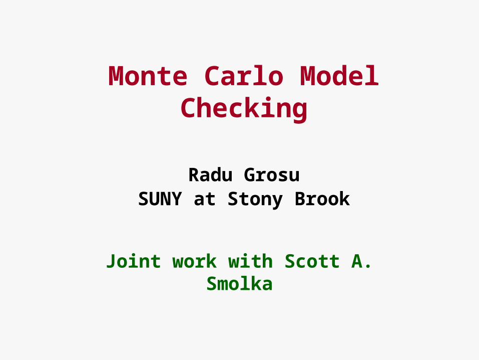
Talk Outline

1. Model Checking

2. Randomized Algorithms

3. LTL Model Checking

4. Probability Theory Primer

5. Monte Carlo Model Checking

6. Implementation & Results

7. Conclusions & Open Problem

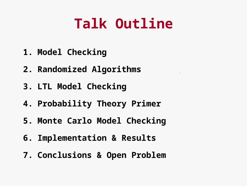
Model Checking

|S ?

Is system S a model of formula φ?

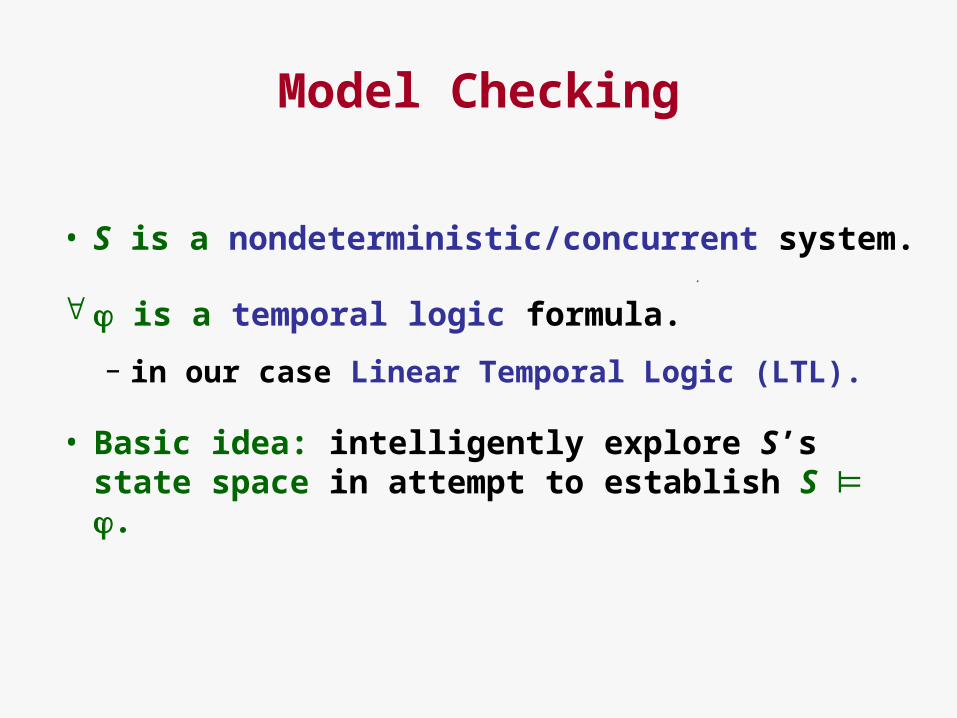
Model Checking

• S is a nondeterministic/concurrent system.

is a temporal logic formula.

– in our case Linear Temporal Logic (LTL).

• Basic idea: intelligently explore S’s state space in attempt to establish S ⊨ .

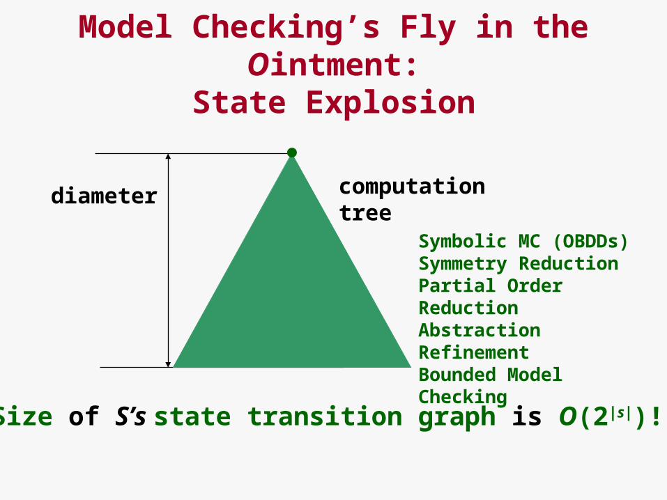
diameter computationtree

Size of S’s state transition graph is O(2|s|)!

Model Checking’s Fly in the Ointment:State Explosion

Symbolic MC (OBDDs)Symmetry ReductionPartial Order ReductionAbstraction RefinementBounded Model Checking

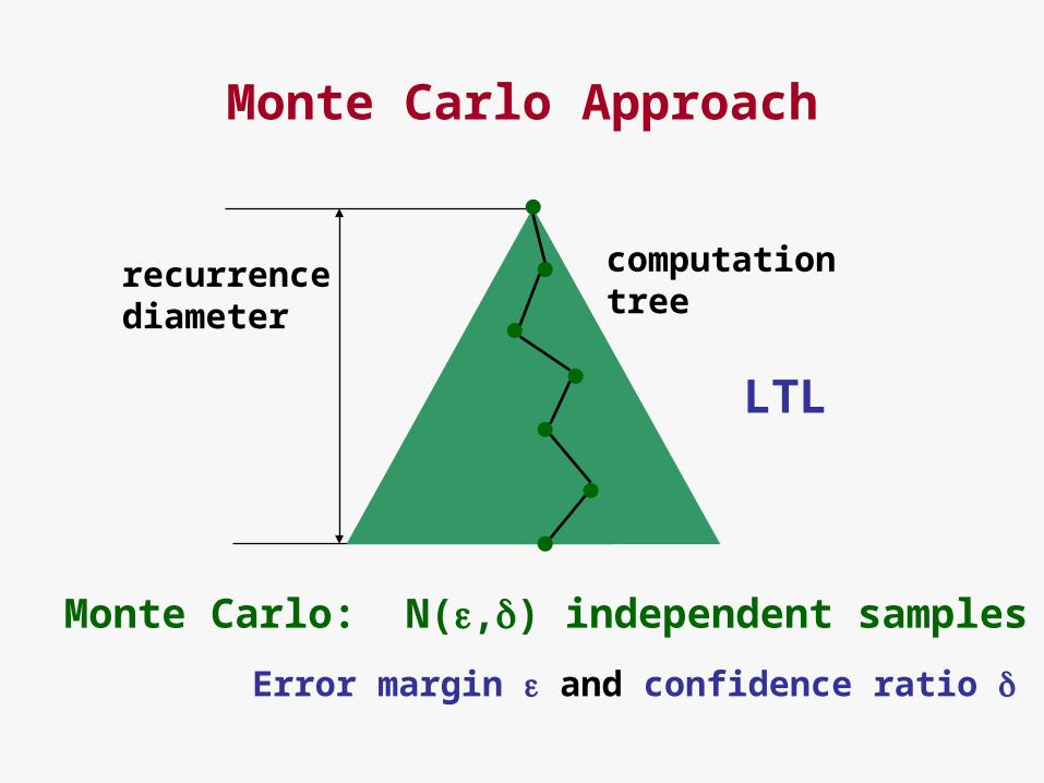
recurrencediameter

computationtree

Monte Carlo: N(,) independent samples

Error margin and confidence ratio

Monte Carlo Approach

LTL

Randomized Algorithms

• Huge impact on CS: (distributed) algorithms, complexity theory, cryptography, etc.

• Takes of next step algorithm may depend on random choice (coin flip).

• Benefits of randomization include simplicity, efficiency, and symmetry breaking.

Randomized Algorithms

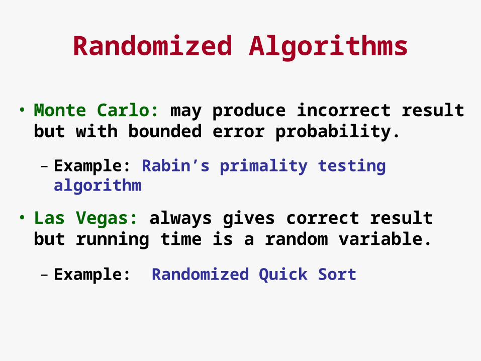
• Monte Carlo: may produce incorrect result but with bounded error probability.

– Example: Rabin’s primality testing algorithm

• Las Vegas: always gives correct result but running time is a random variable.

– Example: Randomized Quick Sort

Linear Temporal Logic

• An LTL formula is made up of atomic propositions p, boolean connectives , , and temporal modalities X (neXt) and U (Until).

• Safety: “nothing bad ever happens” E.g. G( (pc1=cs pc2=cs)) where G is a derived

modality (Globally).

• Liveness: “something good eventually happens” E.g. G( req F serviced ) where F is a derived modality (Finally).

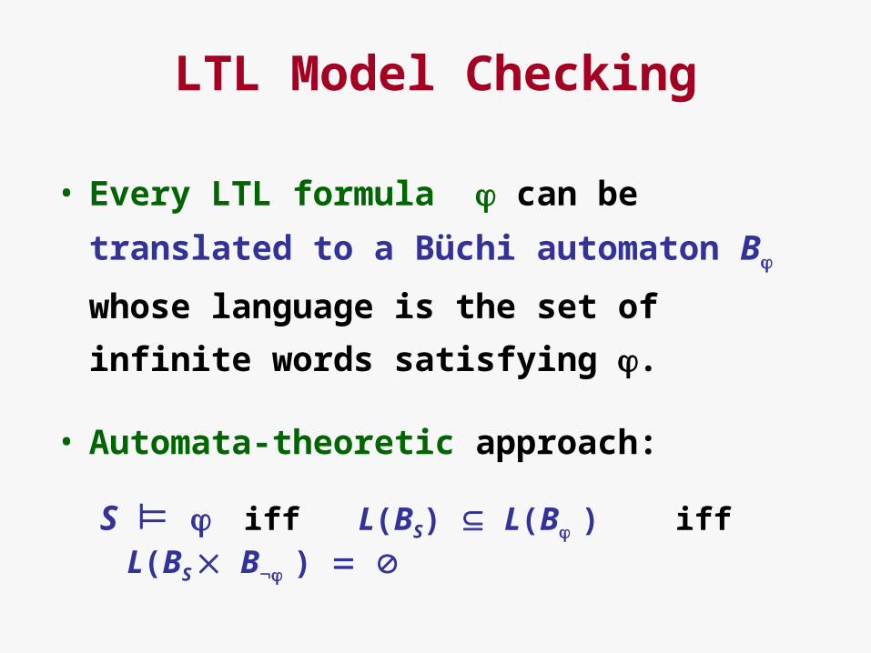
LTL Model Checking

• Every LTL formula can be translated to a

Büchi automaton B whose language is the

set of infinite words satisfying .

• Automata-theoretic approach:

S ⊨ iff L(BS) L(B ) iff L(BS B )

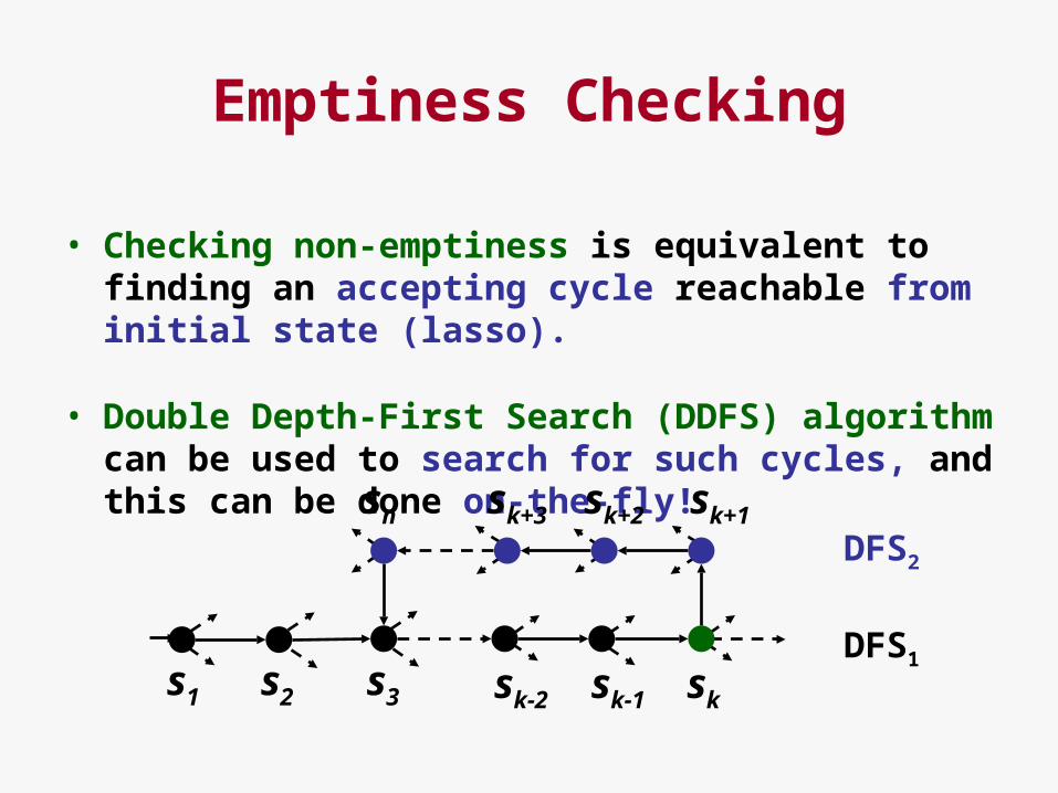
Emptiness Checking

• Checking non-emptiness is equivalent to finding an accepting cycle reachable from initial state (lasso).

• Double Depth-First Search (DDFS) algorithm can be used to search for such cycles, and this can be done on-the-fly!

s1 s2 s3 sksk-2 sk-1

sk+1sk+2sk+3sn

DFS2

DFS1

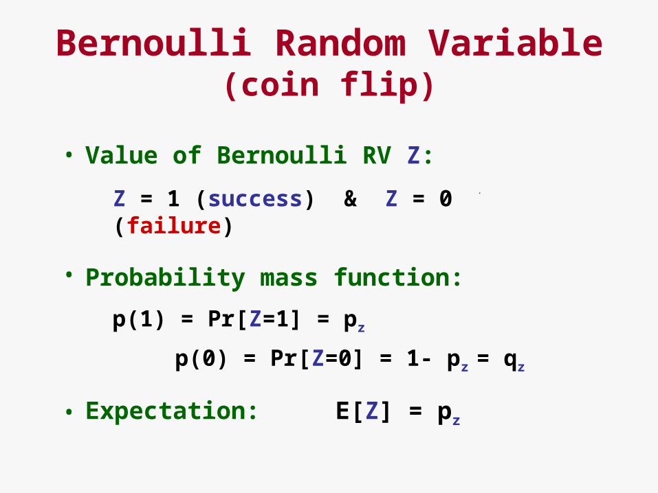
Bernoulli Random Variable(coin flip)

• Value of Bernoulli RV Z:

Z = 1 (success) & Z = 0 (failure)

• Probability mass function:

p(1) = Pr[Z=1] = pz

p(0) = Pr[Z=0] = 1- pz = qz

• Expectation: E[Z] = pz

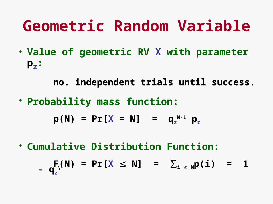
Geometric Random Variable

• Value of geometric RV X with parameter pz:

no. independent trials until success.

• Probability mass function:

p(N) = Pr[X = N] = qzN-1 pz

• Cumulative Distribution Function:

F(N) = Pr[X N] = ∑i Np(i) = 1 - qzN

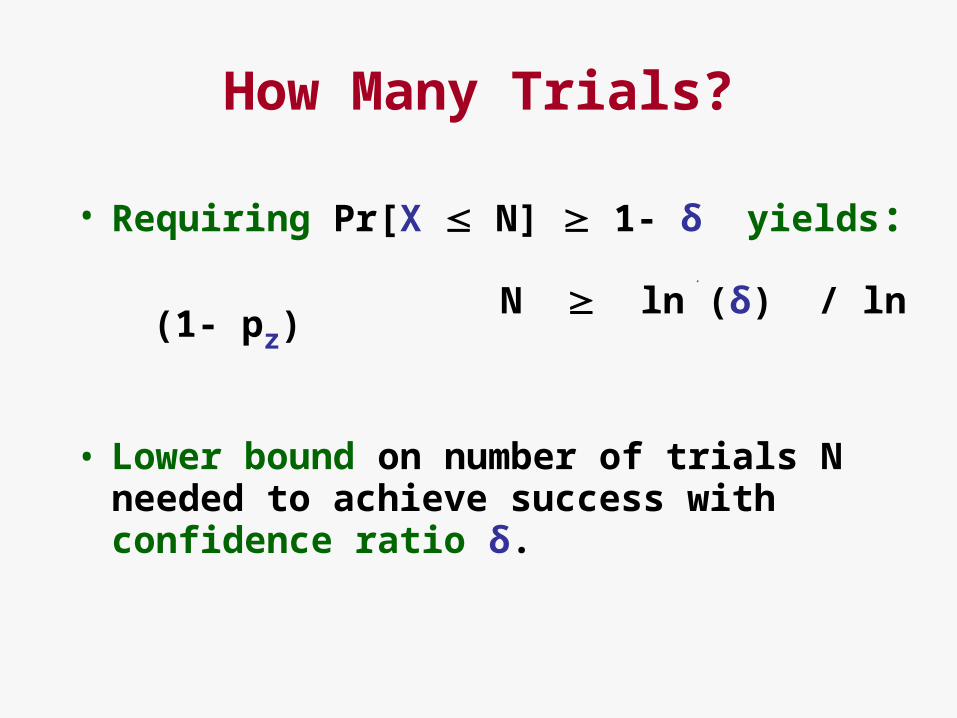
How Many Trials?

• Requiring Pr[X N] 1- δ yields:

N ln (δ) / ln (1- pz)

• Lower bound on number of trials N needed to achieve success with confidence ratio δ.

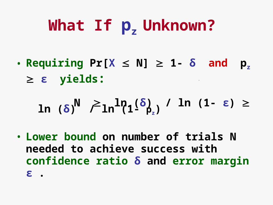
What If pz Unknown?

• Requiring Pr[X N] 1- δ and pz ε yields:

N ln (δ) / ln (1- ε) ln (δ) / ln (1- pz)

• Lower bound on number of trials N needed to achieve success with confidence ratio δ and error margin ε .

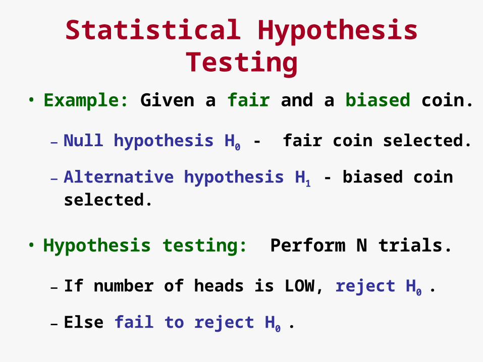
Statistical Hypothesis Testing

• Example: Given a fair and a biased coin.

– Null hypothesis H0 - fair coin selected.

– Alternative hypothesis H1 - biased coin selected.

• Hypothesis testing: Perform N trials.

– If number of heads is LOW, reject H0 .

– Else fail to reject H0 .

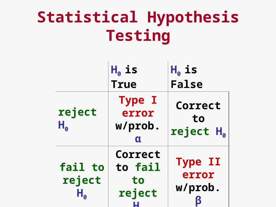
Statistical Hypothesis Testing

H0 is True H0 is False

reject H0

Type I error

w/prob. α

Correct to reject H0

fail to reject H0

Correct to fail to

reject H0

Type II error

w/prob. β

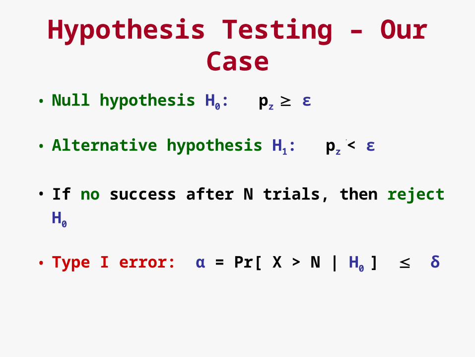
Hypothesis Testing – Our Case

• Null hypothesis H0: pz ε

• Alternative hypothesis H1: pz < ε

• If no success after N trials, then reject H0

• Type I error: α = Pr[ X > N | H0 ] δ

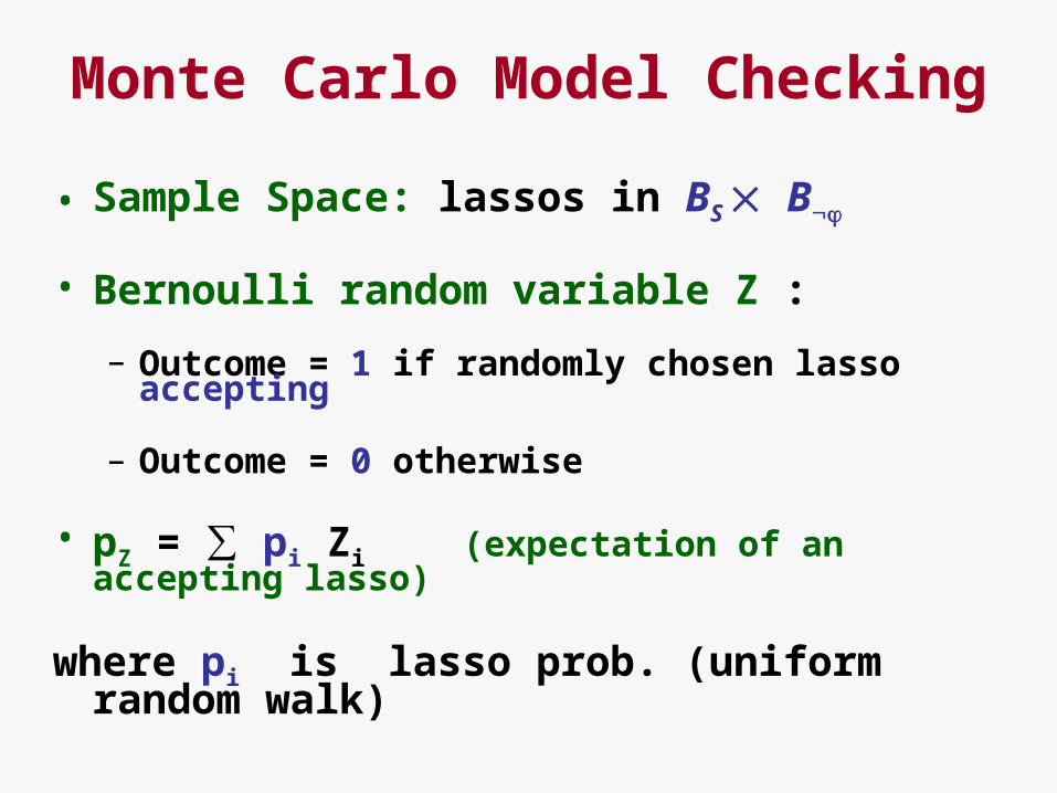
Monte Carlo Model Checking

• Sample Space: lassos in BS B

• Bernoulli random variable Z :

– Outcome = 1 if randomly chosen lasso accepting

– Outcome = 0 otherwise

• pZ = ∑ pi Zi (expectation of an accepting lasso)

where pi is lasso prob. (uniform random walk)

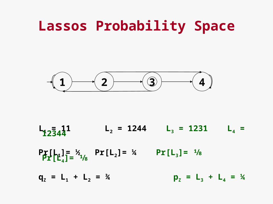
Lassos Probability Space

L1 = 11 L2 = 1244 L3 = 1231 L4 = 12344

Pr[L1]= ½ Pr[L2]= ¼ Pr[L3]= ⅛ Pr[L4]= ⅛

qZ = L1 + L2 = ¾ pZ = L3 + L4 = ¼

1 2 3 4

Monte Carlo Model Checking (MC2)

input: B=(Σ,Q,Q0,δ,F), ε, δ

N = ln (δ) / ln (1- ε)

for (i = 1; i N; i++) if (RL(B) == 1) return (1, error-trace);

return (0, “reject H0 with α = Pr[ X > N | H0 ] < δ”);

where RL(B) performs a uniform random walk through B (storing states encountered in hash table) to obtain a random sample (lasso).

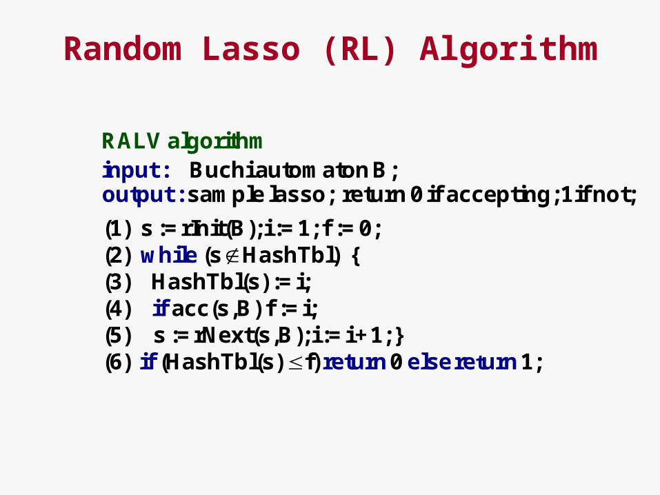
Random Lasso (RL) Algorithm

Buchi automaton B; sample lasso; return 0 if accepting; 1 if not;

(1)

input : output :

while s := rInit(B); i := 1; f := 0;

(2) (s HashTbl) {(3) HashTbl(s) := i;(4) acc

R

(

AL

s,

V al

B) f

gor

:= iif ;

ithm

(5) t

s := rNext(s,B); i := i +1; }(6) (HashTbl(s) f) 0if return elsere urn 1;

Monte Carlo Model Checking

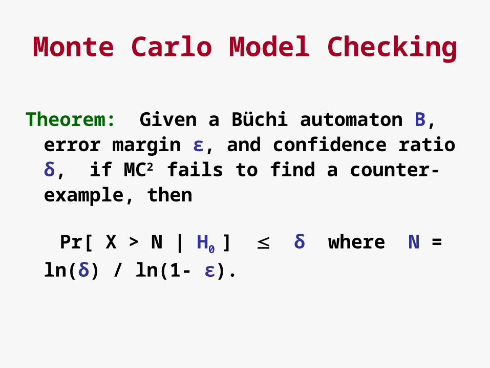
Theorem: Given a Büchi automaton B, error margin ε, and confidence ratio δ, if MC2 fails to find a counter-example, then

Pr[ X > N | H0 ] δ where N = ln(δ) / ln(1- ε).

Monte Carlo Model Checking

Theorem: Given a Büchi automaton B having diameter D, error margin ε, and confidence ratio δ, MC2 runs in time O(N∙D) and uses space O(D), where N = ln(δ) / ln(1- ε).

Cf. DDFS which runs in O(2|S|+|φ|) time

for B = BS B .

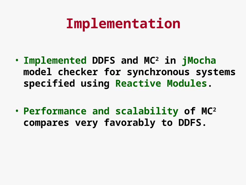
Implementation

• Implemented DDFS and MC2 in jMocha model checker for synchronous systems specified using Reactive Modules.

• Performance and scalability of MC2 compares very favorably to DDFS.

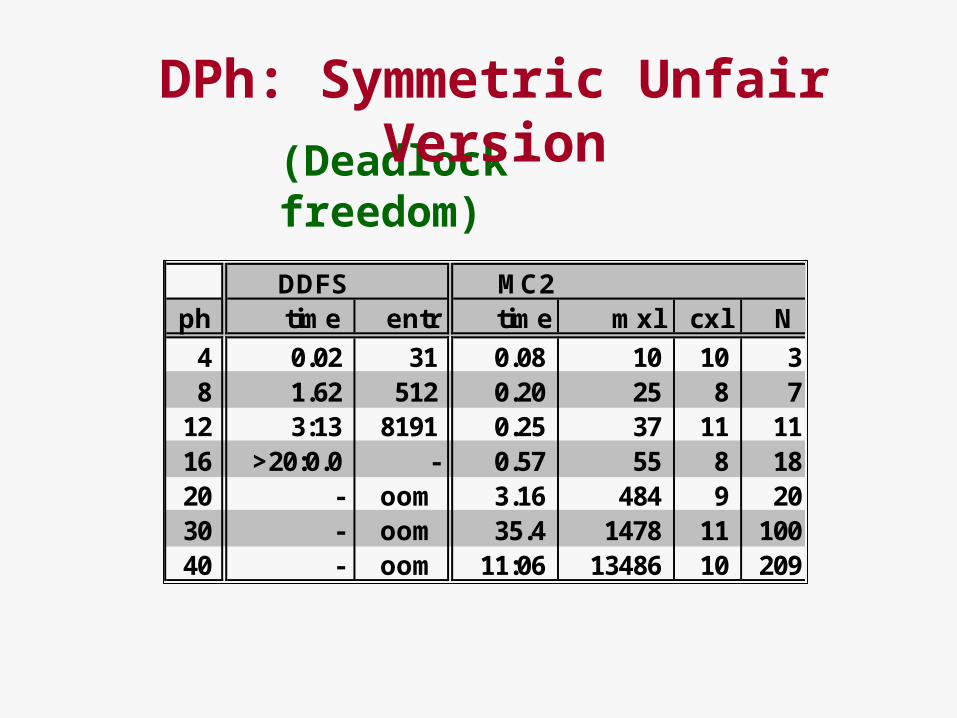
DDFS MC2ph time entr time mxl cxl N

4 0.02 31 0.08 10 10 3 8 1.62 512 0.20 25 8 712 3:13 8191 0.25 37 11 1116 >20:0.0 - 0.57 55 8 1820 - oom 3.16 484 9 2030 - oom 35.4 1478 11 100

40 - oom 11:06 13486 10 209

(Deadlock freedom)

DPh: Symmetric Unfair Version

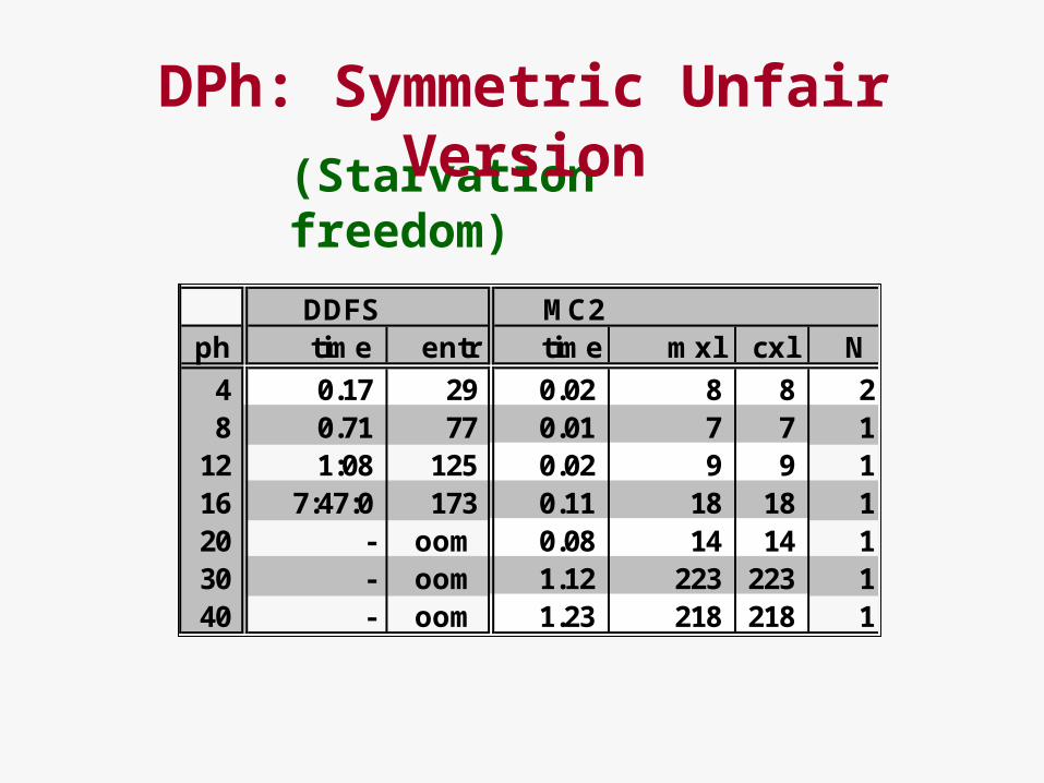
DDFS MC2ph time entr time mxl cxl N

4 0.17 29 0.02 8 8 2 8 0.71 77 0.01 7 7 112 1:08 125 0.02 9 9 116 7:47:0 173 0.11 18 18 120 - oom 0.08 14 14 130 - oom 1.12 223 223 1

40 - oom 1.23 218 218 1

(Starvation freedom)

DPh: Symmetric Unfair Version

DDFS MC2Phi time entries time max avg

4 0:01 178 0:20 49 216 0:03 1772 0:45 116 428 0:58 18244 2:42 365 99

10 16:44 192476 7:20 720 23412 - oom 21:20 1665 56414 - oom 1:09:52 2994 144216 - oom 3:03:40 7358 314418 - oom 6:41:30 13426 589620 - oom 19:02:00 34158 14923

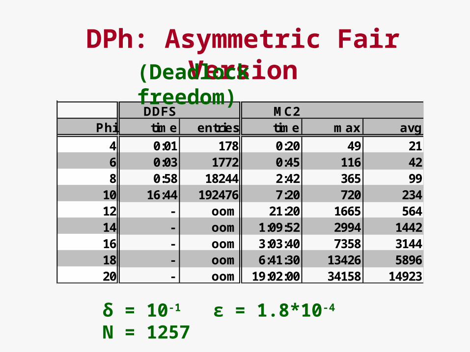
DPh: Asymmetric Fair Version(Deadlock freedom)

δ = 10-1 ε = 1.8*10-4 N = 1257

DDFS MC2Phi time entries time max avg

4 0:01 538 0:20 50 216 0:17 9106 0:46 123 428 7:56 161764 2:17 276 97

10 - oom 7:37 760 24012 - oom 21:34 1682 57014 - oom 1:09:45 3001 136316 - oom 2:50:50 6124 298318 - oom 8:24:10 17962 739020 - oom 22:59:10 44559 17949

DPh: Asymmetric Fair Version (Starvation freedom)

δ = 10-1 ε = 1.8*10-4 N = 1257

Alternative Sampling Strategies

0 1 nn-1

• Multilasso sampling: ignores backedges that do not lead to an accepting lasso.

Pr[Ln]= O(2-n)

• Probabilistic systems: there is a natural way to assign a probability to a RL.

• Input partitioning: partition input into classes that trigger the same behavior (guards).

Related Work

• Heimdahl et al.’s Lurch debugger.

• Mihail & Papadimitriou (and others) use random walks to sample system state space.

• Herault et al. use bounded model checking to compute an (ε,δ)-approx. for “positive LTL”.

• Probabilistic Model Checking of Markov Chains: ETMCC, PRISM, PIOAtool, and others.

Conclusions

• MC2 is first randomized, Monte Carlo algorithm for the classical problem of temporal-logic model checking.

• Future Work: Use BDDs to improve run time. Also, take samples in parallel!

• Open Problem: Branching-Time Temporal Logic (e.g. CTL, modal mu-calculus).