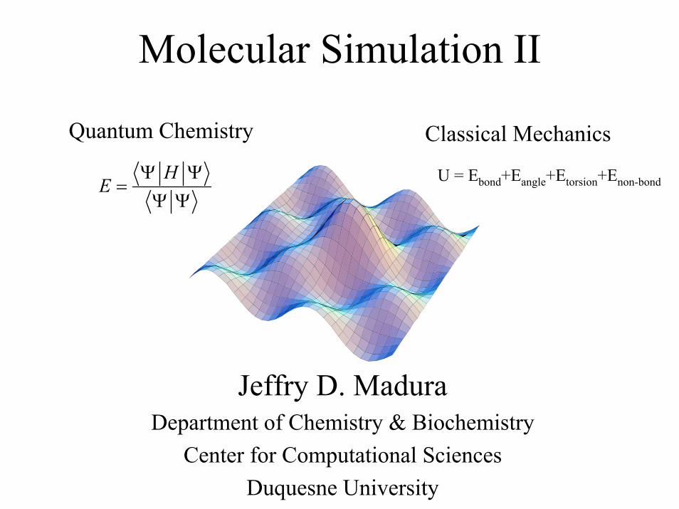
Molecular Simulation II

Quantum Chemistry Classical Mechanics

Jeffry D. MaduraDepartment of Chemistry & Biochemistry

Center for Computational SciencesDuquesne University

HE

Ψ Ψ=

Ψ ΨU = Ebond+Eangle+Etorsion+Enon-bond

Classical Mechanical TreatmentI. Classical Mechanics

a. Implicit treatment of electronsb. Use simple analytical functions (i.e., harmonic springs) c. Use Cartesian coordinates, not the z-matrix

II. Force Fieldsa. Have evolved over timeb. Use different analytical terms and parametersc. Are specific for classes of molecules (proteins,

carbohydrates, nucleic acids, organic molecules, etc.)

Force Field• What is a force field?

– A mathematical expression that describes the dependence of the energy of a molecule on the coordinates of the atoms in the molecule

– Also this sometimes used as another term for potential energy function.

• What are force fields used for?– Structure determination– Conformational energies– Rotational and Pyramidal inversion barriers– Vibrational frequencies– Molecular dynamics

Force Field History• Pre-1970

– Harmonic• 1970

– For molecules with less than 100 atoms one class of force fields went for high accuracy to match experimental results

– The other class of force fields was for macromolecules.

• Present– There are highly accurate force fields designed

for small molecules and there are force fields for studying protein and other large molecules

Force Field• First force fields developed from experimental

data– X-ray– NMR– Microwave

• Current force fields have made use of quantum mechanical calculations– CFF– MMFF94

• There is no single “best” force field

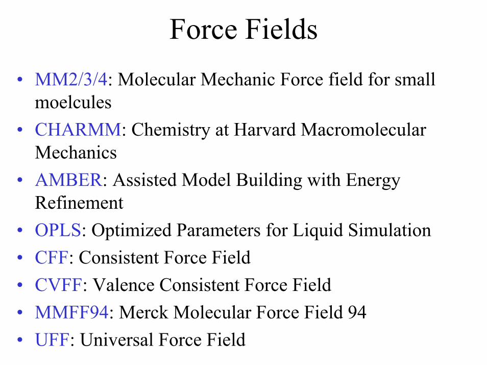
Force Fields• MM2/3/4: Molecular Mechanic Force field for small

moelcules• CHARMM: Chemistry at Harvard Macromolecular

Mechanics• AMBER: Assisted Model Building with Energy

Refinement• OPLS: Optimized Parameters for Liquid Simulation• CFF: Consistent Force Field• CVFF: Valence Consistent Force Field• MMFF94: Merck Molecular Force Field 94• UFF: Universal Force Field

Comparison and Evaluation• Engler, E. M., J. D. Andose and P. v. R. Schleyer (1973) "Critical Evaluation of Molecular Mechanics," J. Am.

Chem. Soc. 95, 8005-8025. Gundertofte, K., J. Palm, I. Pettersson and A. Stamvik (1991) "A Comparison of Conformational Energies Calculated by Molecular Mechanics (MM2(85), Sybyl 5.1, Sybyl 5.21, ChemX) and Semiempirical (AM1 and PM3) Methods," J. Comp. Chem. 12, 200-208.

• Gundertofte, K., T. Liljefors, P-O Norrby, I. Pattesson (1996) "Comparison of Conformational Energies Calculated by Several Molecular Mechanics Methods," J. Comp. Chem. 17, 429-449 (1996).

• Hall, D., and N. Pavitt (1984) "A Appraisal of Molecular Force Fields for the Representation of Polypeptides," J. Comp. Chem. 5, 441-450.

• Hobza, P., M. Kabelac, J. Sponer, P. Mejzlik and J. Vondrasek (1997) "Performance of Empirical Potentials (AMBER, CFF95, CVFF, CHARMM, OPS, POLTEV), Semiemprical Quantum Chemical Methods (AM1, MNDO/M, PM3) and ab initio Hartree-Fock Method for Interaction of DNA Bases: Comparison of Nonempirical Beyond Hartree-Fock Results," J. Comp. Chem. 18, 1136-1150.

• Kini, R. M., and H. J. Evans (1992) "Comparison of Protein Models Minimized by the All-Atom and United Atom Models in the AMBER force Field," J. Biomol. Structure and Dynamics 10, 265-279.

• Roterman, I. K., Gibson, K. D., and Scheraga, H. A. (1989) "A Comparison of the CHARMM, AMBER, and ECEPP/2 Potential for Peptides I." J. Biomol. Struct. and Dynamics 7, 391-419.

• Roterman, I. K., Lambert, M. H., Gibson, K. D., and Scheraga, H. A. (1989) "A Comparison of the CHARMM, AMBER, and ECEPP/2 Potential for Peptides II." J. Biomol. Struct. and Dynamics 7, 421-452.

• Whitlow, M., and M. M. Teeter (1986) "A Empirical Examination of Potential Energy Minimization using the Well-Determined Structure of the Protein Crambin," J. Am. Chem. Soc. 108, 7163-7172.

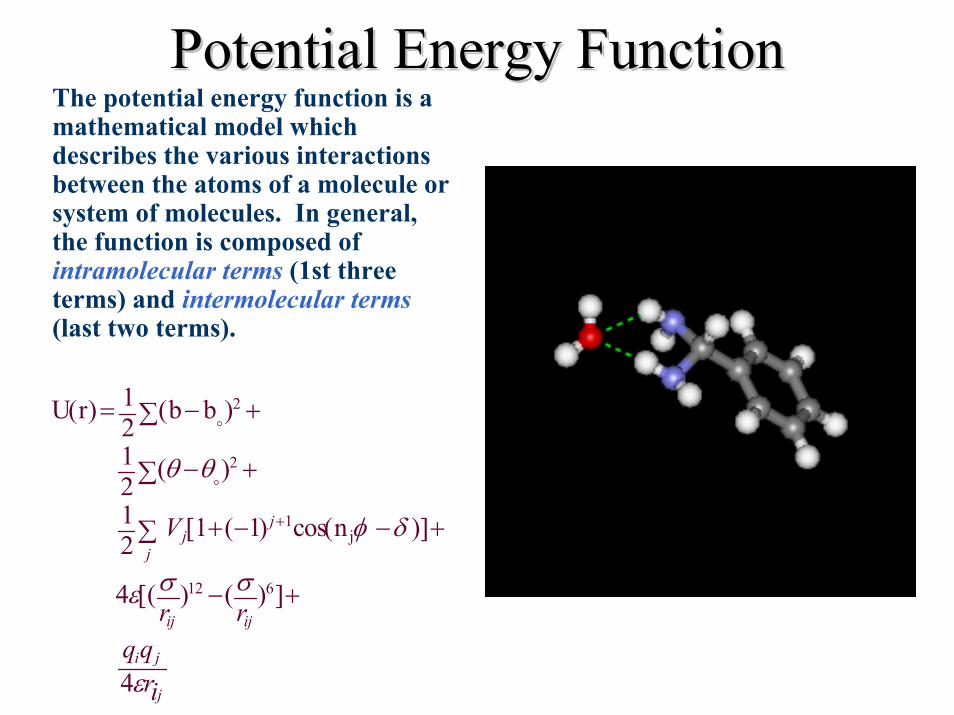
Potential Energy FunctionPotential Energy FunctionThe potential energy function is a mathematical model which describes the various interactions between the atoms of a molecule or system of molecules. In general, the function is composed of intramolecular terms (1st three terms) and intermolecular terms(last two terms).

U r 12

b b

12

cos n

2

2

j

( ) ( )

( )

[ ( ) ( ]

[( ) ( ) ]

= −∑ +

−∑ +

∑ + − − +

− +

+

o

o

)

θ θ

φ δ

ε σ σ

ε

12

1 1

4

4

1

12 6

jj

j

ij ij

i j

j

V

r rq qri

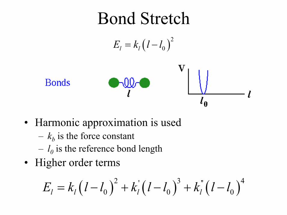
Bond Stretch( )2

0l lE k l l= −

• Harmonic approximation is used– kb is the force constant– l0 is the reference bond length

• Higher order terms

( ) ( ) ( )2 3 4' ''0 0 0l l l lE k l l k l l k l l= − + − + −

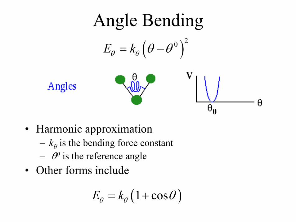
Angle Bending( )20E kθ θ θ θ= −

• Harmonic approximation– kθ is the bending force constant– θ0 is the reference angle

• Other forms include

( )1 cosE kθ θ θ= +

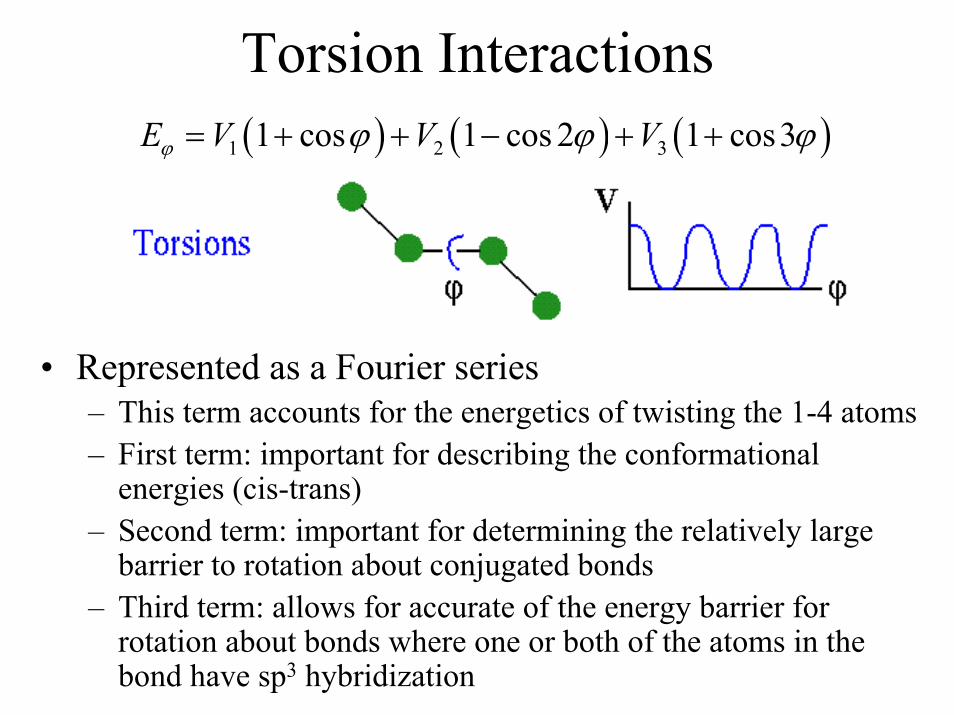
Torsion Interactions( ) ( ) ( )1 2 31 cos 1 cos 2 1 cos3E V V Vϕ ϕ ϕ ϕ= + + − + +

• Represented as a Fourier series– This term accounts for the energetics of twisting the 1-4 atoms– First term: important for describing the conformational

energies (cis-trans)– Second term: important for determining the relatively large

barrier to rotation about conjugated bonds– Third term: allows for accurate of the energy barrier for

rotation about bonds where one or both of the atoms in the bond have sp3 hybridization

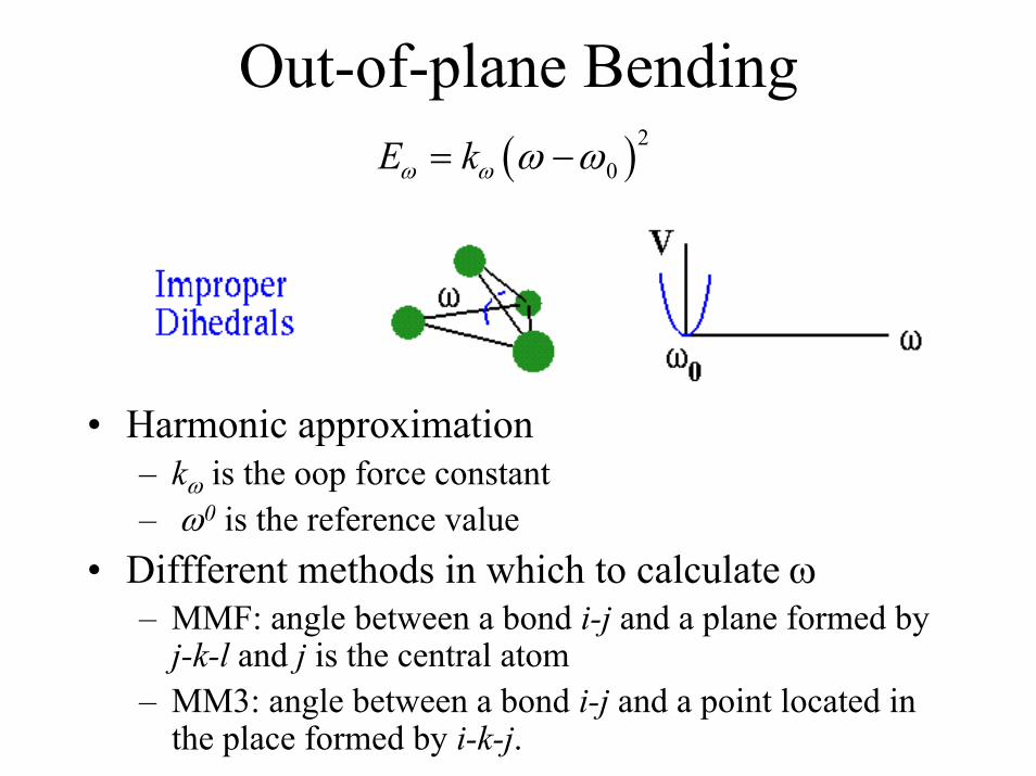
Out-of-plane Bending( )2

0E kω ω ω ω= −

• Harmonic approximation– kω is the oop force constant– ω0 is the reference value

• Diffferent methods in which to calculate ω– MMF: angle between a bond i-j and a plane formed by j-k-l and j is the central atom

– MM3: angle between a bond i-j and a point located in the place formed by i-k-j.

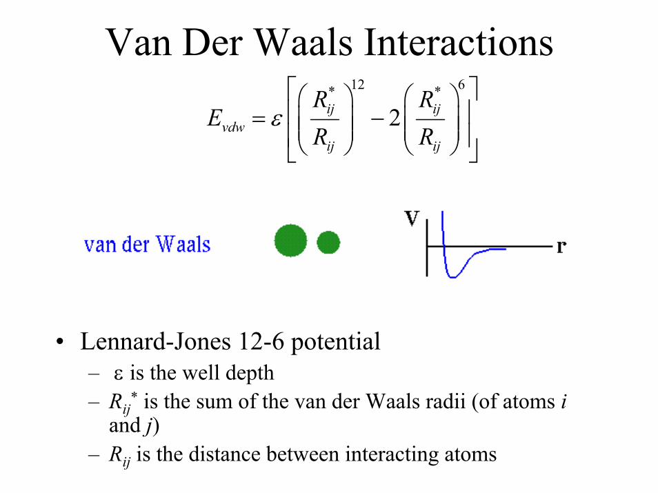
Van Der Waals Interactions12 6* *

2ij ijvdw

ij ij

R RE

R Rε = −

• Lennard-Jones 12-6 potential– ε is the well depth– Rij* is the sum of the van der Waals radii (of atoms i

and j)– Rij is the distance between interacting atoms

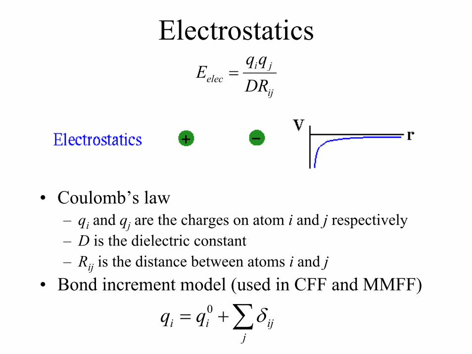
Electrostaticsi j

elecij

q qE

DR=

• Coulomb’s law– qi and qj are the charges on atom i and j respectively– D is the dielectric constant– Rij is the distance between atoms i and j

• Bond increment model (used in CFF and MMFF)0

i i ijj

q q δ= +∑

Charge Classes• Class I

– Calculated directly from experiment• Class II

– Extracted from a quantum mechanical wave function (Mulliken analysis)

• Class III– Extracted from a wave function by analyzing a physical

observable predicted from the wave function. (Electrostatic fitting)

• Class IV– A parameterization procedure to improve class II and III

charges by mapping them to reproduce charge-dependent observables obtained from experiment

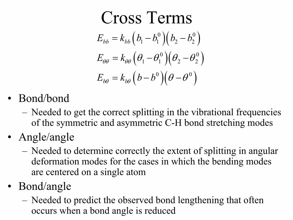
Cross Terms( )( )( )( )( )( )

0 01 1 2 2

0 01 1 2 2

0 0

bb bb

b b

E k b b b b

E k

E k b b

θθ θθ

θ θ

θ θ θ θ

θ θ

= − −

= − −

= − −

• Bond/bond– Needed to get the correct splitting in the vibrational frequencies

of the symmetric and asymmetric C-H bond stretching modes• Angle/angle

– Needed to determine correctly the extent of splitting in angulardeformation modes for the cases in which the bending modes are centered on a single atom

• Bond/angle– Needed to predict the observed bond lengthening that often

occurs when a bond angle is reduced

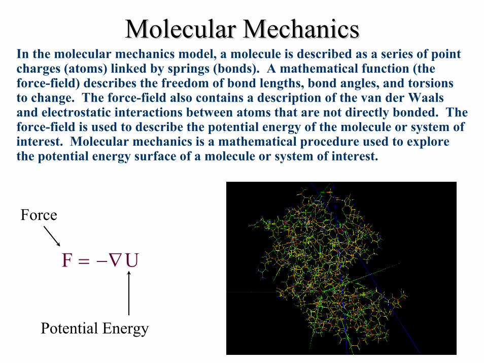
Molecular MechanicsMolecular MechanicsIn the molecular mechanics model, a molecule is described as a series of point charges (atoms) linked by springs (bonds). A mathematical function (the force-field) describes the freedom of bond lengths, bond angles, and torsions to change. The force-field also contains a description of the van der Waalsand electrostatic interactions between atoms that are not directly bonded. The force-field is used to describe the potential energy of the molecule or system of interest. Molecular mechanics is a mathematical procedure used to explore the potential energy surface of a molecule or system of interest.

Force

F U= −∇

Potential Energy

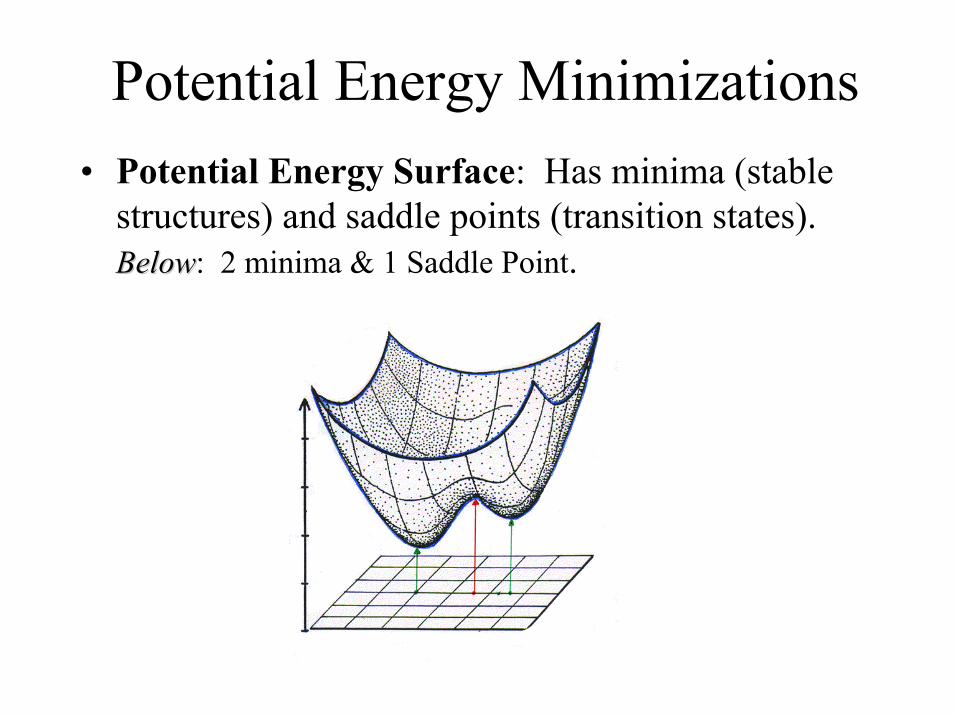
Potential Energy Minimizations• Potential Energy Surface: Has minima (stable

structures) and saddle points (transition states). BelowBelow: 2 minima & 1 Saddle Point.

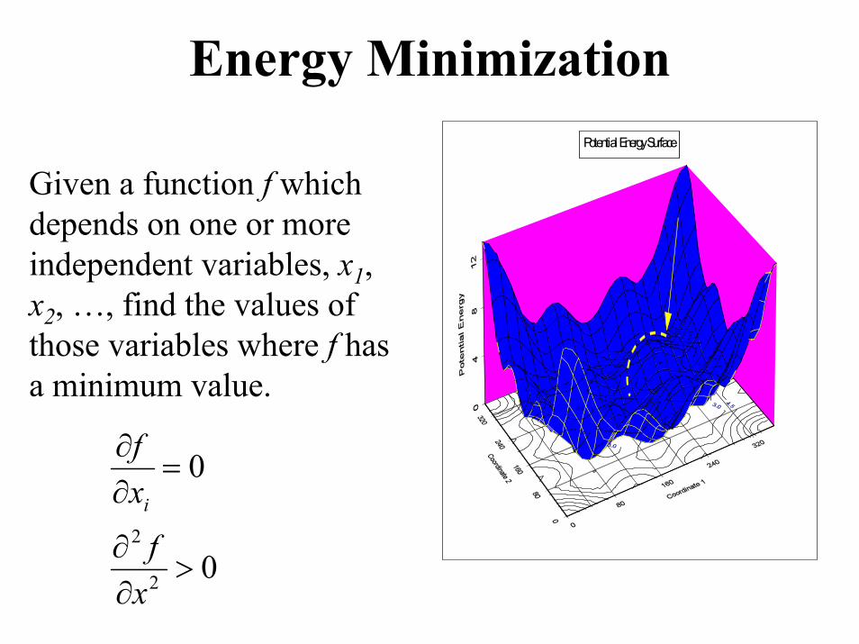
Energy MinimizationPotential Energy Surface

Given a function f which depends on one or more independent variables, x1, x2, …, find the values of those variables where f has a minimum value.

2

2

0

0

i

fx

fx

∂=

∂

∂>

∂

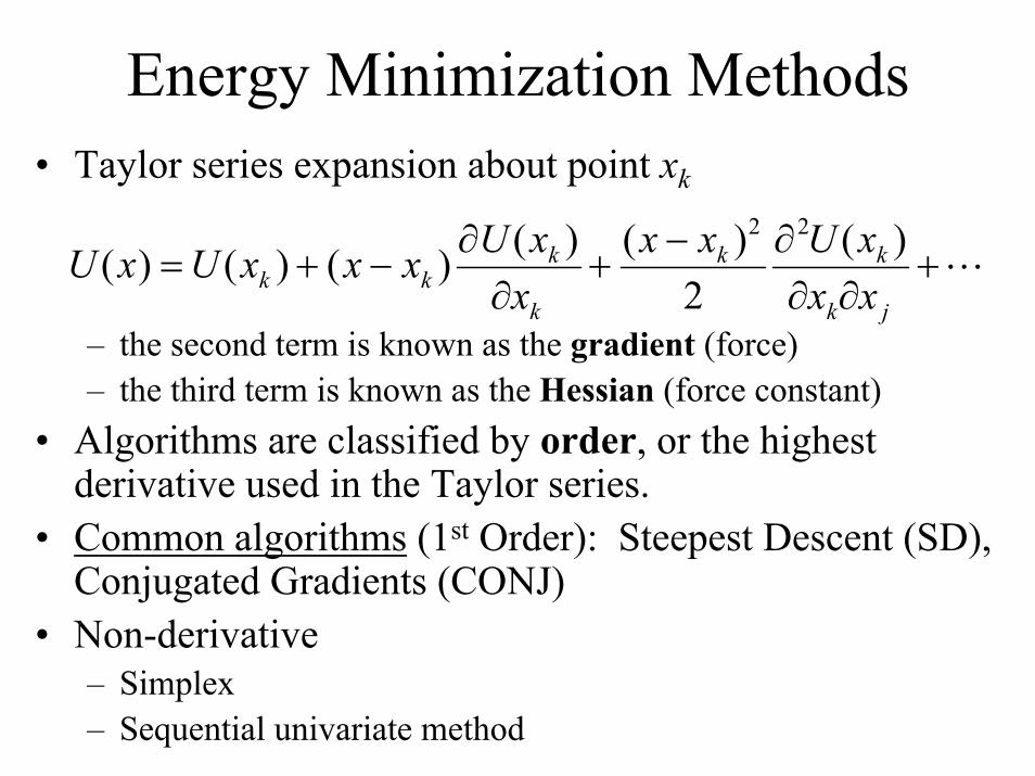
Energy Minimization Methods• Taylor series expansion about point xk

– the second term is known as the gradient (force)– the third term is known as the Hessian (force constant)

• Algorithms are classified by order, or the highest derivative used in the Taylor series.

• Common algorithms (1st Order): Steepest Descent (SD), Conjugated Gradients (CONJ)

• Non-derivative– Simplex– Sequential univariate method

2 2( ) ( ) ( )( ) ( ) ( )2

k k kk k

k k j

U x x x U xU x U x x xx x x

∂ − ∂= + − + +

∂ ∂ ∂L

Energy Minimization Methods• Derivative

– Steepest descents• Moves are made in the direction parallel to the net force

– Conjugate gradient• The gradients and the direction of successive steps are

orthogonal

– Newton-Raphson• Second-order method; both first and second derivatives are

used

– BFGS• Quasi-Newton method (a.k.a. variable metric methods)

build up the inverse Hessian matrix in successive iterations

Energy Minimization Methods– Truncated Newton-Raphson

• Initially follow a descent direction and near the solution solve more accurately using a Newton method.

• Different from QN in that the Hessian is sparse allowing for a faster evaluation

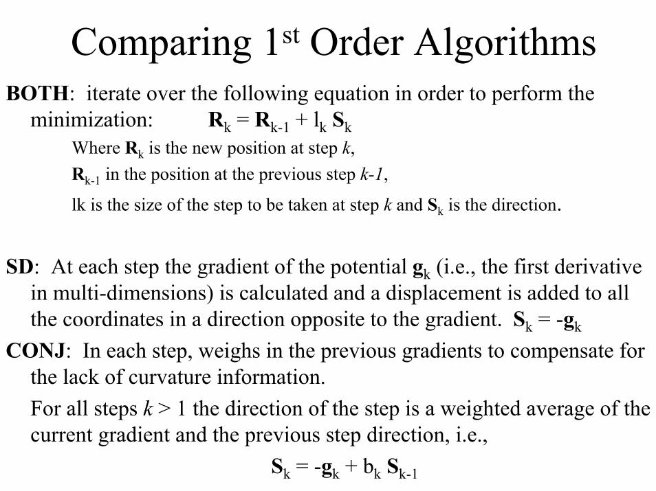
Comparing 1st Order AlgorithmsBOTH: iterate over the following equation in order to perform the

minimization: Rk = Rk-1 + lk SkWhere Rk is the new position at step k, Rk-1 in the position at the previous step k-1,

lk is the size of the step to be taken at step k and Sk is the direction.

SD: At each step the gradient of the potential gk (i.e., the first derivative in multi-dimensions) is calculated and a displacement is added to all the coordinates in a direction opposite to the gradient. Sk = -gk

CONJ: In each step, weighs in the previous gradients to compensate for the lack of curvature information. For all steps k > 1 the direction of the step is a weighted average of the current gradient and the previous step direction, i.e.,

Sk = -gk + bk Sk-1

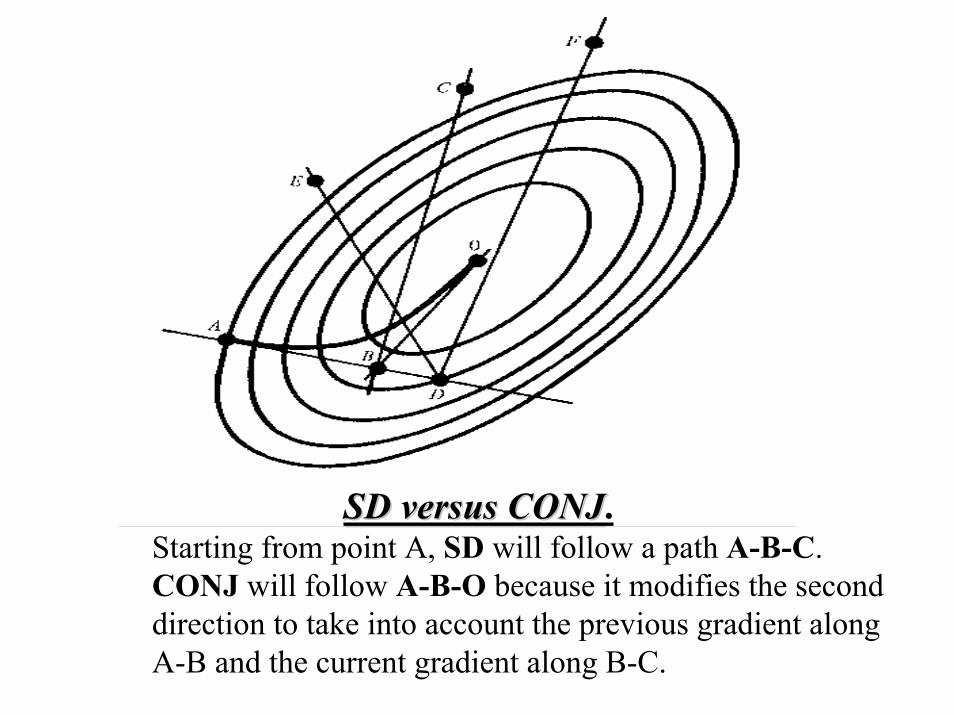
SD versus CONJSD versus CONJ.Starting from point A, SD will follow a path A-B-C. CONJ will follow A-B-O because it modifies the second direction to take into account the previous gradient along A-B and the current gradient along B-C.

Comparison of Methods

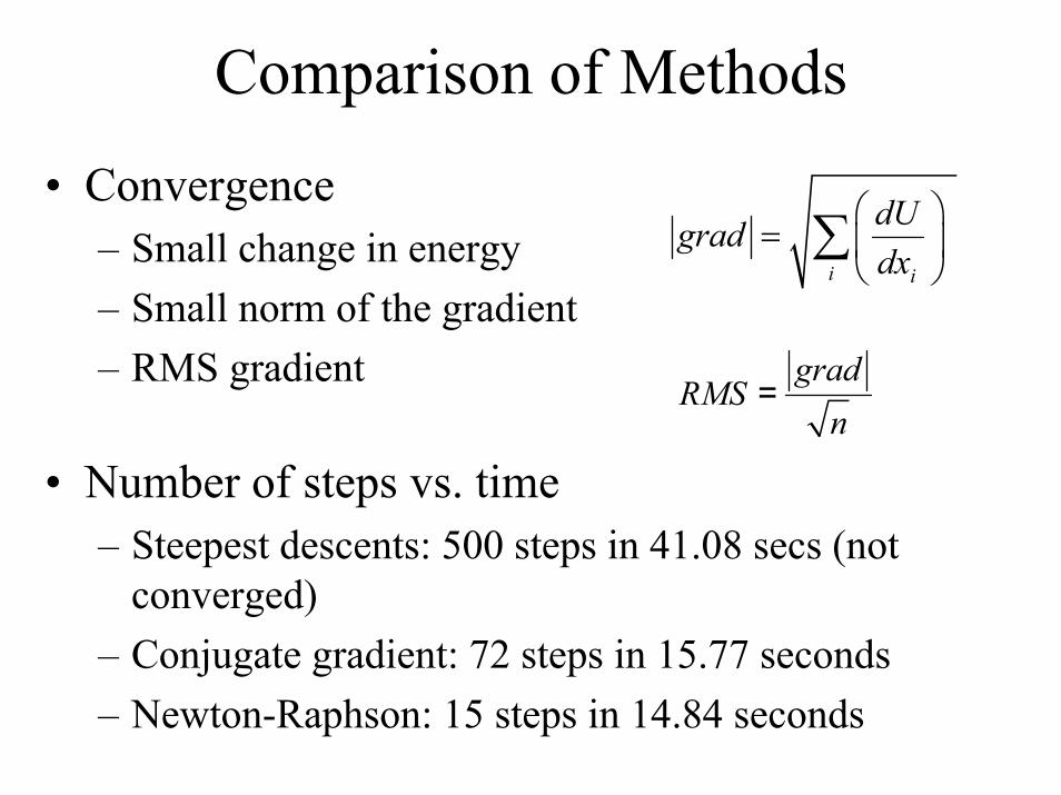
• Convergence– Small change in energy– Small norm of the gradient– RMS gradient

• Number of steps vs. time– Steepest descents: 500 steps in 41.08 secs (not

converged)– Conjugate gradient: 72 steps in 15.77 seconds– Newton-Raphson: 15 steps in 14.84 seconds

i i

dUgraddx

=

∑

gradRMS

n=

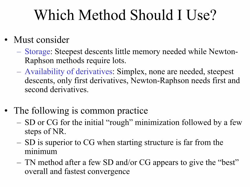
Which Method Should I Use?• Must consider

– Storage: Steepest descents little memory needed while Newton-Raphson methods require lots.

– Availability of derivatives: Simplex, none are needed, steepest descents, only first derivatives, Newton-Raphson needs first and second derivatives.

• The following is common practice– SD or CG for the initial “rough” minimization followed by a few

steps of NR.– SD is superior to CG when starting structure is far from the

minimum– TN method after a few SD and/or CG appears to give the “best”

overall and fastest convergence

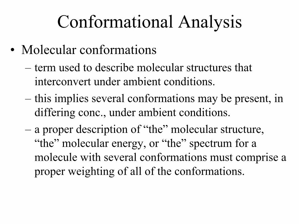
Conformational Analysis• Molecular conformations

– term used to describe molecular structures that interconvert under ambient conditions.

– this implies several conformations may be present, in differing conc., under ambient conditions.

– a proper description of “the” molecular structure, “the” molecular energy, or “the” spectrum for a molecule with several conformations must comprise a proper weighting of all of the conformations.

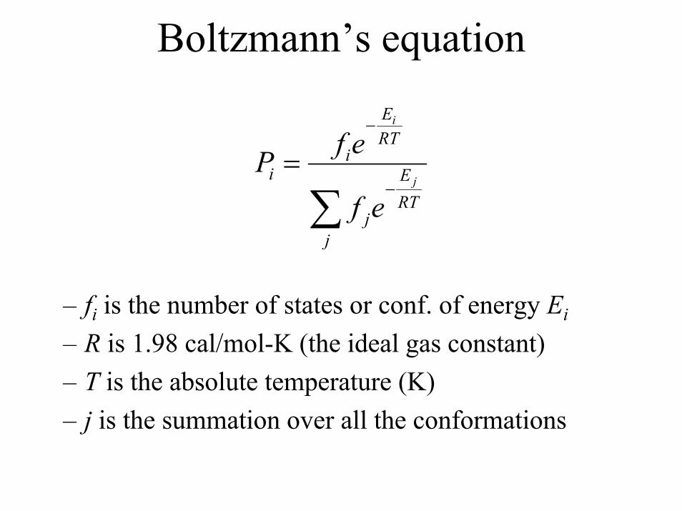
Boltzmann’s equation

i

j

ERT

ii E

RTj

j

f ePf e

−

−=

∑

– fi is the number of states or conf. of energy Ei– R is 1.98 cal/mol-K (the ideal gas constant)– T is the absolute temperature (K)– j is the summation over all the conformations

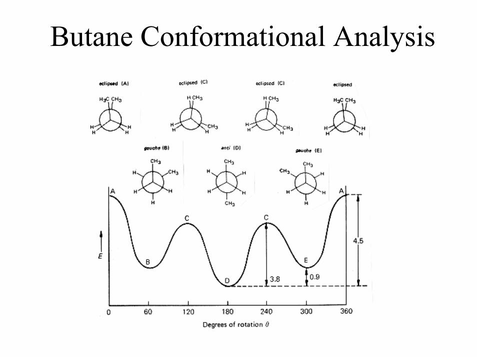
Butane Conformational Analysis

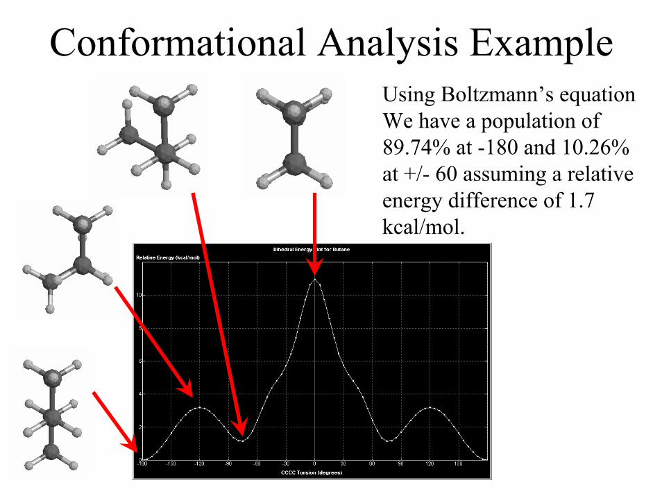
Conformational Analysis ExampleUsing Boltzmann’s equationWe have a population of89.74% at -180 and 10.26%at +/- 60 assuming a relativeenergy difference of 1.7kcal/mol.

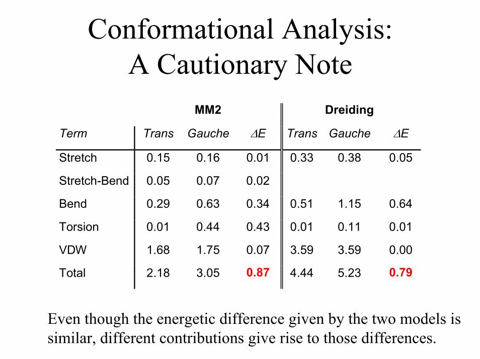
Conformational Analysis:A Cautionary Note

MM2 Dreiding

Term Trans Gauche ∆E Trans Gauche ∆E

Stretch 0.15 0.16 0.01 0.33 0.38 0.05

Stretch-Bend 0.05 0.07 0.02

Bend 0.29 0.63 0.34 0.51 1.15 0.64

Torsion 0.01 0.44 0.43 0.01 0.11 0.01

VDW 1.68 1.75 0.07 3.59 3.59 0.00

Total 2.18 3.05 0.87 4.44 5.23 0.79

Even though the energetic difference given by the two models issimilar, different contributions give rise to those differences.

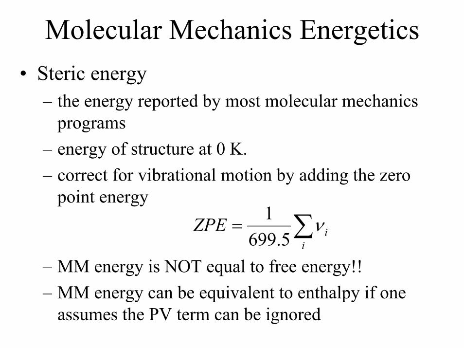
Molecular Mechanics Energetics• Steric energy

– the energy reported by most molecular mechanics programs

– energy of structure at 0 K.– correct for vibrational motion by adding the zero

point energy

– MM energy is NOT equal to free energy!!– MM energy can be equivalent to enthalpy if one

assumes the PV term can be ignored

1699.5 i

i

ZPE ν= ∑

Molecular Mechanics Energy• Strain energy

– Differences in steric energy are oly valid for different conformations or configurations.

– Strain energy permits the comparison between different molecules.

– A “strainless” reference point must be determined.– A particular reference point might be the all trans conformations

of the straight-chain alkanes from methane to hexane (Allingerdefinition).

– These compounds can be used to derive a set of strainlessenergy parameters for constituent parts of molecules.

– Subtracting the strainless energy from the steric energy Allingerand co-workers concluded that the chair cyclohexane has an inherent strain energy due to the presence of 1,4 van der Waalsinteractions between the carbon atom within the ring.

Molecular Mechanics Energy• Interaction energy

– This is the difference between the energies of two isolated species and the energy of the intermolecular complex

– Mathematically this is represented as

( )ie ab a bE E E E= − +

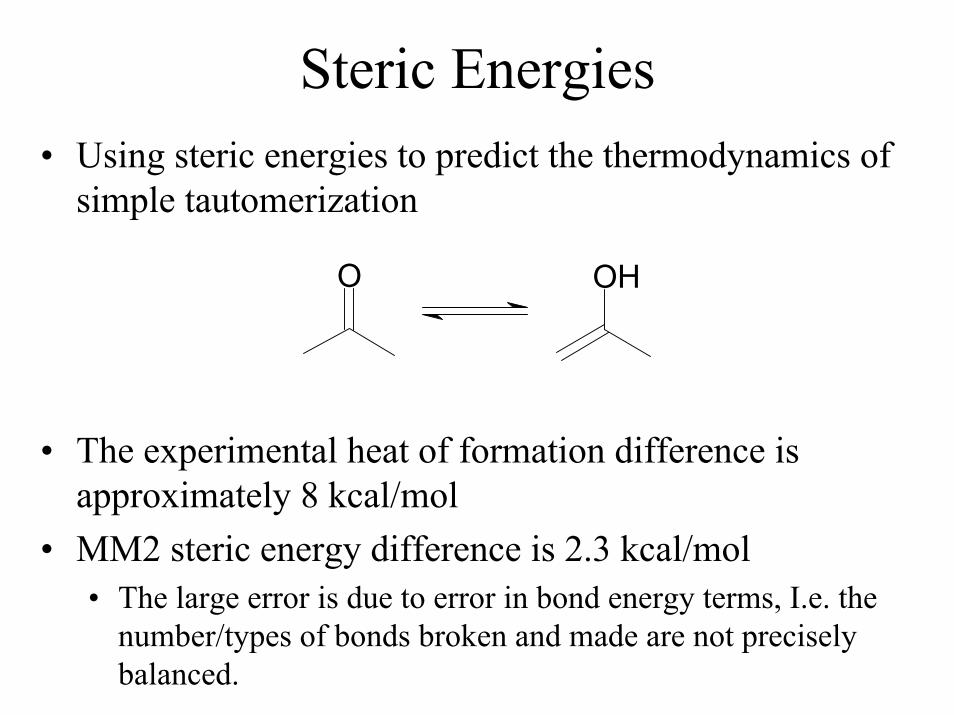
Steric Energies• Using steric energies to predict the thermodynamics of

simple tautomerization

O OH

• The experimental heat of formation difference is approximately 8 kcal/mol

• MM2 steric energy difference is 2.3 kcal/mol• The large error is due to error in bond energy terms, I.e. the

number/types of bonds broken and made are not precisely balanced.

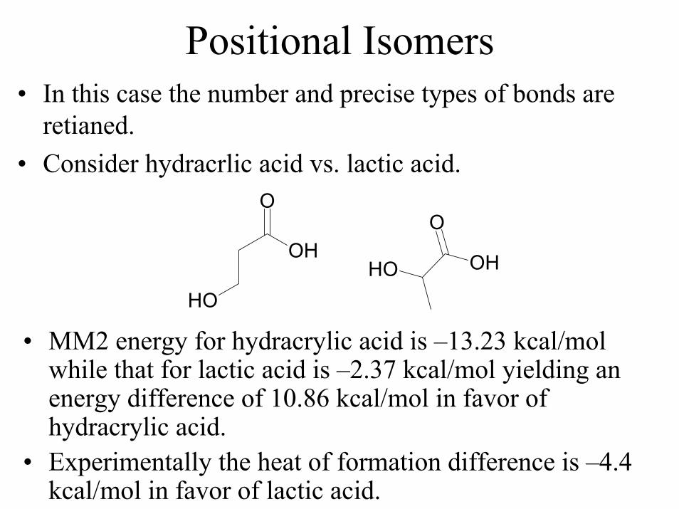
Positional Isomers• In this case the number and precise types of bonds are

retianed.• Consider hydracrlic acid vs. lactic acid.

OH

OH

O

OH OH

O

• MM2 energy for hydracrylic acid is –13.23 kcal/mol while that for lactic acid is –2.37 kcal/mol yielding an energy difference of 10.86 kcal/mol in favor of hydracrylic acid.

• Experimentally the heat of formation difference is –4.4 kcal/mol in favor of lactic acid.

Conformers and Configurational Isomers

• Molecular mechanics can be employed to predict relative energies of conformers and configurational isomers.

• It should not be used on positional isomers or the relative energies of different molecules.

• Molecular mechanics can be used to study the binding between molecules is intermolecular interactions have been appropriately parameterized.

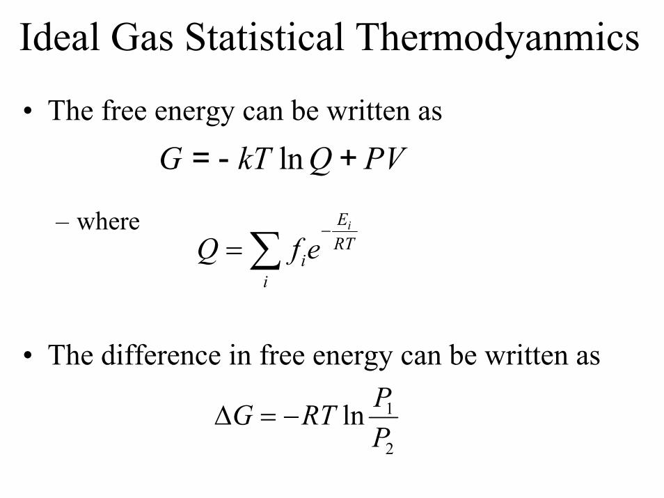
Ideal Gas Statistical Thermodyanmics

• The free energy can be written as

– where

• The difference in free energy can be written as

lnG kT Q PV= - +

iERT

ii

Q f e−

= ∑

1

2

ln PG RTP

∆ = −

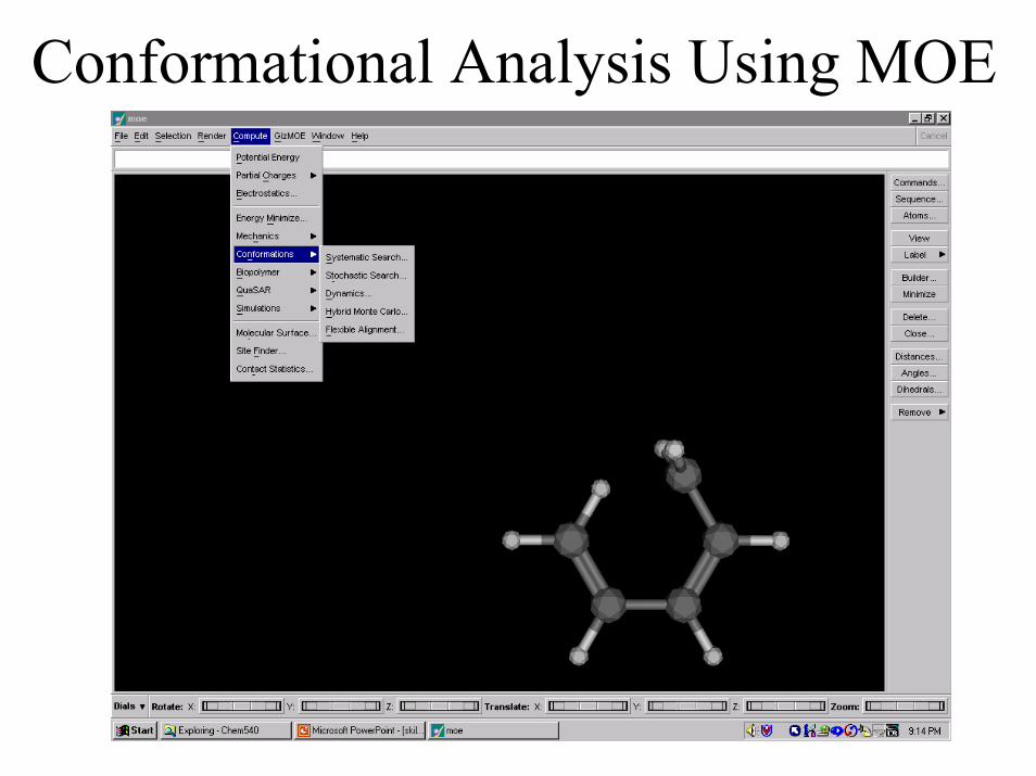
Conformational Analysis Using MOE

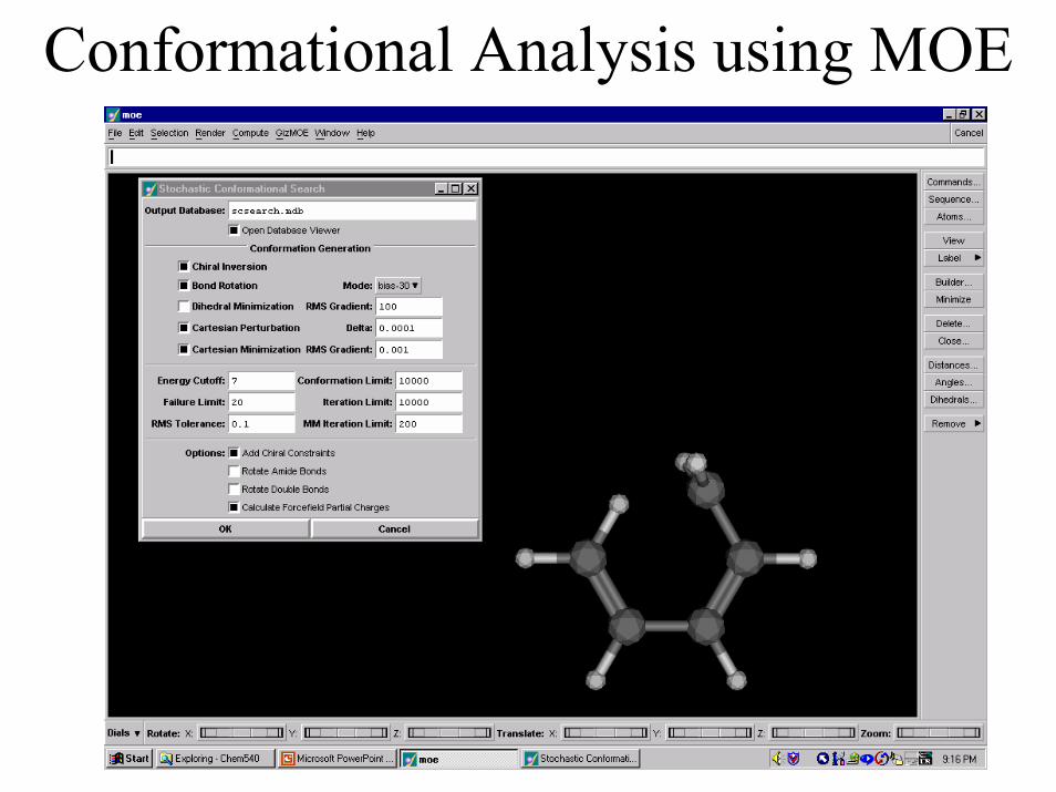
Conformational Analysis using MOE

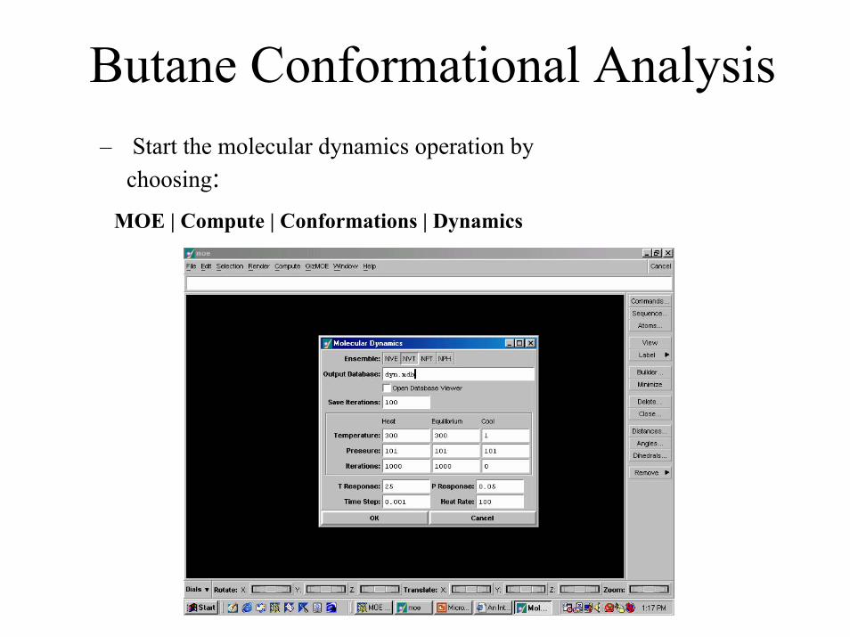
Butane Conformational Analysis– Start the molecular dynamics operation by

choosing: MOE | Compute | Conformations | Dynamics

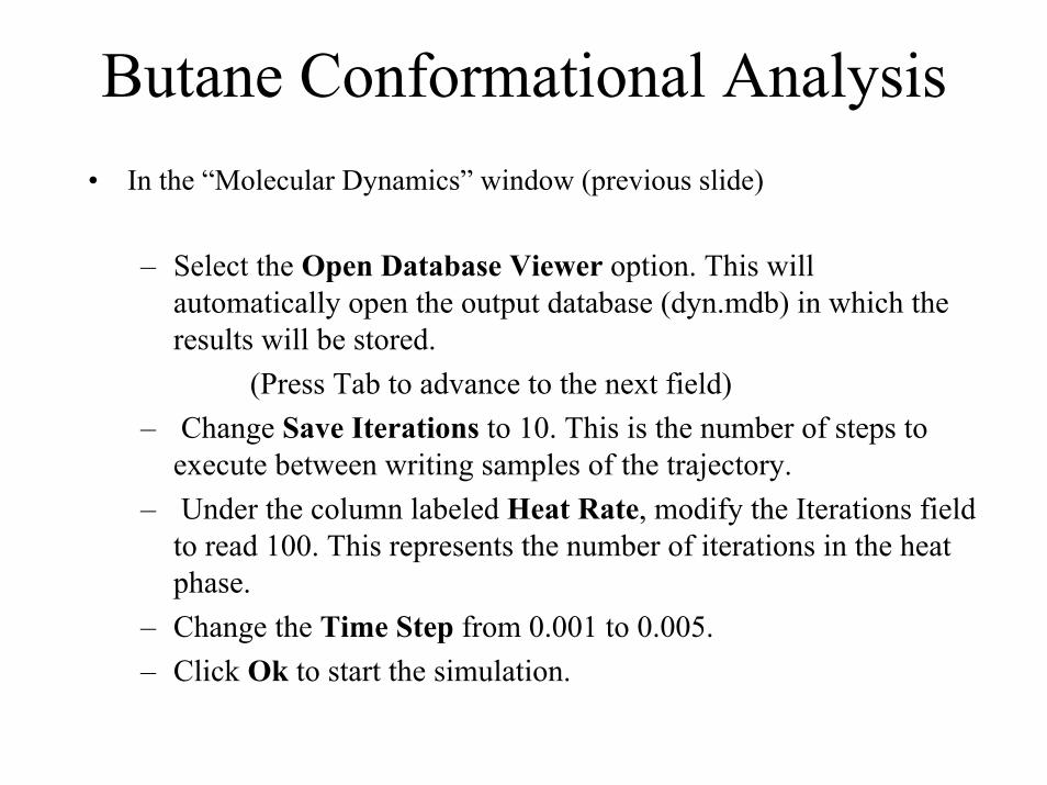
Butane Conformational Analysis• In the “Molecular Dynamics” window (previous slide)

– Select the Open Database Viewer option. This will automatically open the output database (dyn.mdb) in which the results will be stored.

(Press Tab to advance to the next field)– Change Save Iterations to 10. This is the number of steps to

execute between writing samples of the trajectory. – Under the column labeled Heat Rate, modify the Iterations field

to read 100. This represents the number of iterations in the heat phase.

– Change the Time Step from 0.001 to 0.005. – Click Ok to start the simulation.

Butane Conformational Analysis• Once the simulation is complete, you can review the

dynamics simulation as a movie animation: – Open the Dynamics Animator panel in the Database

Viewer:

DBV | File | Dynamics Animator• The MD Animator animates the various

conformations generated by the molecular dynamics run. (next slide)

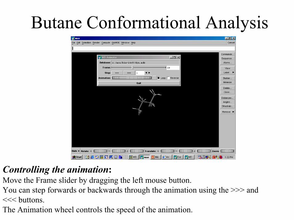
Butane Conformational Analysis

Controlling the animation: Move the Frame slider by dragging the left mouse button. You can step forwards or backwards through the animation using the >>> and <<< buttons. The Animation wheel controls the speed of the animation.