
Moduli of parabolic connections on curves and the...
74
J. ALGEBRAIC GEOMETRY 22 (2013) 407–480 S 1056-3911(2013)00621-9 Article electronically published on February 14, 2013 MODULI OF PARABOLIC CONNECTIONS ON CURVES AND THE RIEMANN-HILBERT CORRESPONDENCE MICHI-AKI INABA Abstract Let (C, t)(t =(t 1 ,...,t n )) be an n-pointed smooth projective curve of genus g and take an element λ =(λ (i) j ) ∈ C nr such that − ∑ i,j λ (i) j = d ∈ Z. For a weight α, let M α C (t, λ) be the moduli space of α-stable (t, λ)-parabolic connections on C and let RP r (C, t) a be the moduli space of representations of the fundamental group π 1 (C \{t 1 ,...,t n }, ∗) with the local monodromy data a for a certain a ∈ C nr . Then we prove that the morphism RH : M α C (t, λ) → RP r (C, t) a determined by the Riemann-Hilbert correspondence is a proper surjective bimeromorphic morphism. As a corollary, we prove the geometric Painlev´ e property of the isomonodromic deformation defined on the moduli space of parabolic connections. 1. Introduction Let C be a smooth projective curve over C and t 1 ,...,t n be distinct points of C . For an algebraic vector bundle E on C and a logarithmic connec- tion ∇ : E → E ⊗ Ω 1 C (t 1 + ··· + t n ), ker ∇ an | C\{t 1 ,...,t n } becomes a local system on C \{t 1 ,...,t n } and corresponds to a representation of the fun- damental group π 1 (C \{t 1 ,...,t n }, ∗), where ∇ an is the analytic connection corresponding to ∇. The correspondence (E, ∇) → ker ∇ an | C\{t 1 ,...,t n } is said to be the Riemann-Hilbert correspondence. If l ⊂ E| t i is a subspace satisfying res t i (∇)(l) ⊂ l, then ∇ induces a connection ∇ : E → E ⊗ Ω 1 C (t 1 + ··· + t n ), where E := ker(E → (E| t i /l)) and res t i (∇) means the residue of ∇ at t i . We say (E , ∇ ) is the elementary transform of (E, ∇) along t i by l. Note that ker ∇ an | C\{t 1 ,...,t n } ∼ = ker(∇ ) an | C\{t 1 ,...,t n } . Received August 4, 2009 and, in revised form, November 25, 2010 and July 30, 2012. c 2013 University Press, Inc. 407 Licensed to Kyoto University. Prepared on Tue Jul 2 01:23:02 EDT 2013 for download from IP 130.54.110.71. License or copyright restrictions may apply to redistribution; see http://www.ams.org/license/jour-dist-license.pdf
Transcript of Moduli of parabolic connections on curves and the...
J. ALGEBRAIC GEOMETRY22 (2013) 407–480S 1056-3911(2013)00621-9Article electronically published on February 14, 2013
MODULI OF PARABOLIC CONNECTIONSON CURVES AND THE RIEMANN-HILBERT
CORRESPONDENCE
MICHI-AKI INABA
Abstract
Let (C, t) (t = (t1, . . . , tn)) be an n-pointed smooth projective curve of
genus g and take an element λ = (λ(i)j ) ∈ Cnr such that −
∑i,j λ
(i)j =
d ∈ Z. For a weight α, let MαC (t,λ) be the moduli space of α-stable
(t,λ)-parabolic connections on C and let RPr(C, t)a be the modulispace of representations of the fundamental group π1(C \{t1, . . . , tn}, ∗)with the local monodromy data a for a certain a ∈ Cnr. Then we provethat the morphism RH : Mα
C (t,λ) → RPr(C, t)a determined by theRiemann-Hilbert correspondence is a proper surjective bimeromorphicmorphism. As a corollary, we prove the geometric Painleve property ofthe isomonodromic deformation defined on the moduli space of parabolicconnections.
1. Introduction
Let C be a smooth projective curve over C and t1, . . . , tn be distinct points
of C. For an algebraic vector bundle E on C and a logarithmic connec-
tion ∇ : E → E ⊗ Ω1C(t1 + · · · + tn), ker∇an|C\{t1,...,tn} becomes a local
system on C \ {t1, . . . , tn} and corresponds to a representation of the fun-
damental group π1(C \ {t1, . . . , tn}, ∗), where ∇an is the analytic connection
corresponding to ∇. The correspondence (E,∇) �→ ker∇an|C\{t1,...,tn} is said
to be the Riemann-Hilbert correspondence. If l ⊂ E|ti is a subspace satisfying
resti(∇)(l) ⊂ l, then ∇ induces a connection ∇′ : E′ → E′⊗Ω1C(t1+ · · ·+ tn),
where E′ := ker(E → (E|ti/l)) and resti(∇) means the residue of ∇ at ti. We
say (E′,∇′) is the elementary transform of (E,∇) along ti by l. Note that
ker∇an|C\{t1,...,tn}∼= ker(∇′)an|C\{t1,...,tn}.
Received August 4, 2009 and, in revised form, November 25, 2010 and July 30, 2012.
c©2013 University Press, Inc.
407
Licensed to Kyoto University. Prepared on Tue Jul 2 01:23:02 EDT 2013 for download from IP 130.54.110.71.
License or copyright restrictions may apply to redistribution; see http://www.ams.org/license/jour-dist-license.pdf
408 MICHI-AKI INABA
We put
Λ(n)r (d) :=
⎧⎨⎩(λ
(i)j )1≤i≤n
0≤j≤r−1 ∈ Cnr
∣∣∣∣∣∣d+∑i,j
λ(i)j = 0
⎫⎬⎭
for integers d, r, n with r > 0, n > 0. We write t = (t1, . . . , tn) and take an
element λ ∈ Λ(n)r (d).
Definition 1.1. We say (E,∇, {l(i)∗ }1≤i≤n) is a (t,λ)-parabolic connection
of rank r if
(1) E is a rank r algebraic vector bundle on C,
(2) ∇ : E → E ⊗ Ω1C(t1 + · · ·+ tn) is a connection, and
(3) for each ti, l(i)∗ is a filtration E|ti = l
(i)0 ⊃ l
(i)1 ⊃ · · · ⊃ l
(i)r−1 ⊃ l
(i)r = 0
such that dim(l(i)j /l
(i)j+1) = 1 and (resti(∇)−λ
(i)j idE|ti )(l
(i)j ) ⊂ l
(i)j+1 for
j = 0, . . . , r − 1.
The filtration l(i)∗ (1 ≤ i ≤ n) is said to be a parabolic structure on the
vector bundle E. For a parabolic connection (E,∇, {l(i)j }), the elementary
transform of (E,∇) along ti by l(i)j determines another parabolic connection.
Then an elementary transform gives a transformation Elm(i)j on the set of
isomorphism classes of parabolic connections; see section 3, (3) for the pre-
cise definition of Elm(i)j . Then the Riemann-Hilbert correspondence gives a
bijection RH between the set
(†){(E,∇, {l(i)j }) : parabolic connection of rank r
}/∼
and the set
(††) {ρ : π1(C \ {t1, . . . , tn}, ∗) → GLr(C) : representation} / ∼=,
where ∼ is the equivalence relation generated by x ∼ Elml(i)j
(x), (E,∇, {l(i)j })
∼ (E,∇, {l(i)j })⊗OC(tk) and (E,∇, {l(i)j }) ∼ (E,∇, {l′(i)j }) and / ∼=means the
isomorphism classes. The bijectivity of RH immediately follows from the the-
ory of Deligne [4]. Indeed take any representation ρ : π1(C \{t1, . . . , tn}, ∗) →GLr(C). Then ρ corresponds to a locally constant sheaf V on C \{t1, . . . , tn}.By [4, II, Proposition 5.4], there is a unique pair (E,∇) of a vector bundle E
and a connection ∇ : E → E⊗Ω1C(t1+· · ·+tn) such that all the eigenvalues of
resti(∇) lie in {λ ∈ C|0 ≤ Re(λ) < 1} and ker∇an|C\{t1,...,tn}∼= V. We can
take a parabolic structure {l(i)j } on E compatible with the connection∇. Then
(E,∇, {l(i)j }) becomes a parabolic connection and RH([(E,∇, {l(i)j })]) = ρ.
So RH is surjective. Let (E,∇, {l(i)j }) be a (t,λ)-parabolic connection and
(E′,∇′, {(l′)(i)j }) be a (t,λ′)-parabolic connection such that RH([(E,∇, {l(i)j })])
Licensed to Kyoto University. Prepared on Tue Jul 2 01:23:02 EDT 2013 for download from IP 130.54.110.71.
License or copyright restrictions may apply to redistribution; see http://www.ams.org/license/jour-dist-license.pdf
MODULI OF PARABOLIC CONNECTIONS ON CURVES 409
= RH([(E′,∇′, {(l′)(i)j })]), namely ker∇an|C\{t1,...,tn}∼=ker(∇′)an|C\{t1,...,tn}.
By Proposition 3.1, there is a (t,μ)-parabolic connection (E1,∇1, {(l1)(i)j })and a (t,μ′)-parabolic connection (E′
1,∇′1, {(l′1)
(i)j }) such that (E,∇, {l(i)j }) ∼
(E1,∇1, {(l1)(i)j }), (E′,∇′, {(l′)(i)j }) ∼ (E′1,∇′
1, {(l′1)(i)j }) and 0 ≤ Re(μ
(i)j )
< 1, 0 ≤ Re((μ′)(i)j ) < 1 for any i, j. Since ker∇an
1 |C\{t1,...,tn}∼=
ker(∇′1)
an|C\{t1,...,tn}, we can see by [4, II, Proposition 5.4], that (E1,∇1) ∼=(E′
1,∇′1). So we have (E,∇, {l(i)j }) ∼ (E1,∇1, {(l1)(i)j }) ∼ (E′
1,∇′1, {(l′1)
(i)j })
∼ (E′,∇′, {(l′)(i)j }). Thus we obtain the injectivity of RH.
Unfortunately, we cannot expect an appropriate algebraic structure on the
moduli space of the elements [(E,∇, {l(i)j })] in the set (†); so, it is natural
to consider the moduli space of isomorphism classes of parabolic connections
in the moduli theoretic description of the Riemann-Hilbert correspondence.
However, we must consider a stability when we construct the moduli of para-
bolic connections as an appropriate space, so we set MαC (t,λ) as the moduli
space of α-stable parabolic connections; see Theorem 2.1 and Definition 2.1
for the precise definition of MαC (t,λ). Next we consider the moduli space
RPr(C, t)a of certain equivalence classes of representations of the fundamental
group π1(C \ {t1, . . . , tn}, ∗). Here two representations are equivalent if their
semisimplifications are isomorphic. (There is not an appropriate moduli space
of the isomorphism classes of the representations of the fundamental group.)
For a construction of a good moduli space containing all the representations,
we must consider such an equivalence relation; see section 2 for the precise
definition of RPr(C, t)a. The most crucial part of the main result (Theorem
2.2) is that the morphism RH : MαC (t,λ) −→ RPr(C, t)a determined by the
Riemann-Hilbert correspondence is a proper surjective bimeromorphic mor-
phism. This theorem was proved in [7] for C = P1 and r = 2. However
there were certain difficulties to generalize this fact to the case of general
C and r.
One of the most important motivations to consider such a theorem is the
search for a geometric description of the differential equation determined by
the isomonodromic deformation; see section 8 for the precise definition of
the isomonodromic deformation. This differential equation is said to be the
Schlesinger equation for C = P1, the Garnier equation for C = P1 and r = 2,
and the Painleve VI equation for C = P1, r = 2 and n = 4. M. Jimbo,
T. Miwa and K. Ueno give in [12] and [13] an explicit description of the
Schlesinger equation. In this paper, we will constrct a space M with a mor-
phism π : M → T such that there is a differential equation on M with respect
to a time variable t ∈ T which is determined by the isomonodromic defor-
mation. If we fix a point t0 ∈ T , π−1(t0) should become a space of initial
Licensed to Kyoto University. Prepared on Tue Jul 2 01:23:02 EDT 2013 for download from IP 130.54.110.71.
License or copyright restrictions may apply to redistribution; see http://www.ams.org/license/jour-dist-license.pdf
410 MICHI-AKI INABA
conditions of the differential equation determined by the isomonodromic de-
formation. Take any point x ∈ π−1(t0) and consider the analytic continuation
γ starting at x and πγ coming back to the initial point t0 such that γ is a
solution of the differential equation determined by the isomonodromic defor-
mation. Then γ should come back to a point of π−1(t0). We will generalize
this property to the geometric Painleve property. Roughly speaking, the geo-
metric Painleve property is the property of the space where the differential
equation is defined and any analytic continuation of a solution of the differen-
tial equation stays in the space; see Definition 2.4 for the precise definition of
the geometric Painleve property. In fact we will take M as the moduli space
MαC/T (t, r, d) of α-stable parabolic connections and π : Mα
C/T (t, r, d) → T
as the structure morphism. For example let us assume that C = P1 and
take an α-stable parabolic connection x = (E,∇, {l(i)j }) such that E ∼= O⊕rP1 .
Let γ : [0, 1] → MαP×T/T (t, r, 0) be a path starting at x and πγ ends at
π(x) such that γ is a solution of the differential equation determined by the
isomonodromic deformation. Then the ending point γ(1) corresponds to an
α-stable parabolic connection (E′,∇′, {(l′)(i)j }), but E′ may not be trivial.
So we recognize that it is not enough to consider only trivial vector bundles
with a connection. We should also consider non-trivial vector bundles with a
connection.
Our aim here is to construct a space where the isomonodromic deformation
is defined and has the geometric Painleve property over every value of λ. (It
is not difficult to construct such a space over generic λ, but it is difficult
to construct over special λ.) In fact, that space is nothing but the moduli
space of α-stable parabolic connections and the result is given in Theorem 2.3,
which is essentially a corollary of Theorem 2.2. Here note that the properness
of the morphism RH is very essential in the proof of Theorem 2.3. The
geometric Painleve property immediately implies the usual analytic Painleve
property. So we can say that Theorem 2.3 gives a most clear proof of the
Painleve property of the isomonodromic deformation. As is well known, the
solutions of the Painleve equation have the Painleve property, which is in some
sense the property characterizing the Painleve equation (and there were many
proofs of the Painleve property). So the usual analytic Painleve property
plays an important role in the theory of the Painleve equation, but we can
see from the definition that the “geometric Painleve property” is much more
important from the viewpoint of the description of the geometric picture of
the isomonodromic deformation.
To prove the main results, this paper consists of several sections. In section
4, we prove the existence of the moduli space of stable parabolic connections.
Licensed to Kyoto University. Prepared on Tue Jul 2 01:23:02 EDT 2013 for download from IP 130.54.110.71.
License or copyright restrictions may apply to redistribution; see http://www.ams.org/license/jour-dist-license.pdf
MODULI OF PARABOLIC CONNECTIONS ON CURVES 411
An algebraic moduli space of parabolic connections was essentially consid-
ered by D. Arinkin and S. Lysenko in [1], [2] and [3] and they showed that
the moduli space of parabolic connections on P1 of rank 2 with n = 4 for
generic λ is isomorphic to the space of initial conditions of the Painleve VI
equation constructed by K. Okamoto [16]. For special λ, we should consider
a certain stability condition to construct an appropriate moduli space of par-
abolic connections. In the case of C = P1 and r = 2, K. Iwasaki, M.-H. Saito
and the author already considered in [7] the moduli space of stable parabolic
connections and they proved in [8] that the moduli space of stable parabolic
connections on P1 of rank 2 with n = 4 is isomorphic to the space of initial
conditions of the Painleve VI equation constructed by K. Okamoto for all
λ. An analytic construction of the moduli space of stable parabolic connec-
tions for general C and r = 2 was given by H. Nakajima in [14]. However,
in our aim, the algebraic construction of the moduli space is necessary. The
morphism RH determined by the Riemann-Hilbert correspondence is quite
transcendental, which is explicitly shown in the case of C = P1, r = 2 and
n = 4 in [8]. This statement makes sense only if we construct the moduli
spaces MαC (t,λ) and RPr(C, t)a algebraically. Moduli of logarithmic connec-
tions without parabolic structure are constructed in [15]. For the proof of
Theorem 2.1, we do not use the method in [17]. We construct MαC/T (t, r, d)
as a subscheme of the moduli space of parabolic Λ1D-triples constructed in [7].
We also use this embedding in the proof of the properness of RH in Theorem
2.2.
In section 5, we prove that the moduli space of stable parabolic connec-
tions is an irreducible variety. For the proof, we need certain complicated
calculations and this part is a new difficulty, which did not appear in [7].
In section 6, we consider the morphism RH determined by the Riemann-
Hilbert correspondence and prove the surjectivity and properness of RH.
This is the essential part of the proof of Theorem 2.2. Notice that for generic
λ, any (t,λ)-parabolic connection is irreducible and so all (t,λ)-parabolic
connections are stable. Moreover we can easily see that the moduli space
MαC (t,λ) of parabolic connections for generic λ is analytically isomorphic via
the Riemann-Hilbert correspondence to the moduli space RPr(C, t)a of rep-
resentations of the fundamental group π1(C \ {t1, . . . , tn}, ∗). However, for
special λ, several parabolic connections may not be stable and the stability
condition depends on α. So we can see that the surjectivity of RH is not
trivial at all for special λ, because for a point [ρ] ∈ RPr(C, t)a, we must find
a parabolic connection corresponding to [ρ] which is α-stable. Moreover, the
moduli space MαC (t,λ) of α-stable parabolic connections is smooth, but the
moduli space RPr(C, t)a of representations of the fundamental group becomes
Licensed to Kyoto University. Prepared on Tue Jul 2 01:23:02 EDT 2013 for download from IP 130.54.110.71.
License or copyright restrictions may apply to redistribution; see http://www.ams.org/license/jour-dist-license.pdf
412 MICHI-AKI INABA
singular. So the morphism RH : MαC (t,λ) → RPr(C, t)a is more complicated
in the case of special λ than the case of generic λ. We first prove the sur-
jectivity of RH in Proposition 6.1. In this proof, we use the Langton’s type
theorem in the case of parabolic connections. This idea was already used in
[7]. Secondly, we prove in Proposition 6.2 that every fiber of RH is compact
by using an embedding of MαC (t,λ) into a certain compact moduli space. In
this proof, we cannot use the idea given in [7], so we develop a new tech-
nique again. Finally we obtain the properness of RH by the lemma given by
A. Fujiki.
In section 7, we construct a canonical symplectic form on the moduli space
MαC (t,λ) of α-stable parabolic connections. Combined with the fact that
RH gives an analytic resolution of singularities of RPr(C, t)a, we can say
that RPr(C, t)a has symplectic singularities (for special a) and RH gives a
symplectic resolution of singularities. For the case of r = 2, H. Nakajima
constructed the moduli space MαC (t,λ) as a hyper-Kahler manifold and it
obviously has a holomorphic symplectic structure. Such a construction for
general r is also an important problem, although we do not treat it here.
In section 8, we first give in Proposition 8.1 an algebraic construction of
the differential equation on MαC/T (t, r, d) determined by the isomonodromic
deformation. Finally we complete the proof of Theorem 2.3.
2. Main results
Let C be a smooth projective curve of genus g. We put
Tn :=
⎧⎨⎩(t1, . . . , tn) ∈
n︷ ︸︸ ︷C × · · · × C
∣∣∣∣∣∣ ti �= tj for i �= j
⎫⎬⎭
for a positive integer n. For integers d, r with r > 0, recall the definition of
Λ(n)r (d) given in the introduction and the definition of (t,λ)-parabolic con-
nection for (t,λ) ∈ Tn × Λ(n)r (d) in Definition 1.1.
Remark 2.1. Take a (t,λ)-parabolic connection (E,∇, {l(i)j }). By condi-
tion (3) of Definition 1.1, we have
degE = deg(det(E)) = −n∑
i=1
resti(∇detE) = −n∑
i=1
r−1∑j=0
λ(i)j = d.
Take rational numbers
0 < α(i)1 < α
(i)2 < · · · < α(i)
r < 1
for i = 1, . . . , n satisfying α(i)j �= α
(i′)j′ for (i, j) �= (i′, j′).
Licensed to Kyoto University. Prepared on Tue Jul 2 01:23:02 EDT 2013 for download from IP 130.54.110.71.
License or copyright restrictions may apply to redistribution; see http://www.ams.org/license/jour-dist-license.pdf
MODULI OF PARABOLIC CONNECTIONS ON CURVES 413
Definition 2.1. A parabolic connection (E,∇, {l(i)∗ }1≤i≤n) is α-stable
(resp. α-semistable) if for any proper non-zero subbundle F ⊂ E satisfying
∇(F ) ⊂ F ⊗ Ω1C(t1 + · · ·+ tn), the inequality
degF +∑n
i=1
∑rj=1 α
(i)j dim((F |ti ∩ l
(i)j−1)/(F |ti ∩ l
(i)j ))
rankF
<
(resp. ≤)
degE +∑n
i=1
∑rj=1 α
(i)j dim(l
(i)j−1/l
(i)j )
rankE
holds.
Remark 2.2. Assume that α = (α(i)j ) satisfies the condition: For any
integer r′ with 0 < r′ < rank(E) and for any (ε(i)j )i=1,...,n
j=1,...,rank(E) with ε(i)j ∈
{0, 1} and∑r
j=1 ε(i)j = r′ for any i,
n∑i=1
rank(E)∑j=1
α(i)j (r′ − rank(E)ε
(i)j ) /∈ Z.
Then a parabolic connection (E,∇, {l(i)j }) isα-stable if and only if (E,∇, {l(i)j })is α-semistable.
Let T be a smooth algebraic scheme which is a smooth covering of the
moduli stack of n-pointed smooth projective curves of genus g over C and
take a universal family (C, t1, . . . , tn) over T .Theorem 2.1. There exists a relative fine moduli scheme
MαC/T (t, r, d) → T × Λ(n)
r (d)
of α-stable parabolic connections of rank r and degree d, which is smooth and
quasi-projective. The fiber MαCx(tx,λ) over (x,λ) ∈ T ×Λ
(n)r (d) is the moduli
space of α-stable (tx,λ)-parabolic connections whose dimension is 2r2(g−1)+
nr(r − 1) + 2 if it is non-empty.
Definition 2.2. Take an element λ ∈ Λ(n)r (d). We call λ special if
(1) λ(i)j − λ
(i)k ∈ Z for some i and j �= k, or
(2) there exists an integer s with 0 < s < r and a subset {ji1, . . . , jis} ⊂{0, . . . , r − 1} for each 1 ≤ i ≤ n such that
n∑i=1
s∑k=1
λ(i)
jik∈ Z.
We call λ resonant if it satisfies condition (1) above. Let (E,∇, {l(i)j }) be a
(t,λ)-parabolic connection such that λ does not satisfy condition (2)
above. Then (E,∇, {l(i)j }) is irreducible. Here we say a (tx,λ)-connection
(E,∇E, {l(i)j }) is reducible if there is a non-trivial subbundle 0 �= F � E
Licensed to Kyoto University. Prepared on Tue Jul 2 01:23:02 EDT 2013 for download from IP 130.54.110.71.
License or copyright restrictions may apply to redistribution; see http://www.ams.org/license/jour-dist-license.pdf
414 MICHI-AKI INABA
such that ∇E(F ) ⊂ F ⊗ Ω1Cx((t1)x + · · · + (tn)x). We say (E,∇E , {l(i)j }) is
irreducible if it is not reducible. We call λ ∈ Λ(n)r (d) generic if it is not special.
Fix a point x ∈ T . Then the fundamental group π1(Cx\{(t1)x, . . . , (tn)x}, ∗)is generated by cycles α1, β1, . . . , αg, βg and loops γi around ti for 1 ≤ i ≤ n
whose relation is given by
g∏j=1
α−1j β−1
j αjβj
n∏i=1
γi = 1.
So the fundamental group is isomorphic to a free group generated by 2g+n−1
free generators. Then the space
Hom(π1(Cx \ {(t1)x, . . . , (tn)x}, ∗), GLr(C)
)of representations of the fundamental group becomes an affine variety isomor-
phic to GLr(C)2g+n−1 and GLr(C) acts on this space by the adjoint action.
We define
RPr(Cx, tx) := Hom(π1(Cx \ {(t1)x, . . . , (tn)x}, ∗), GLr(C)
)//GLr(C)
as the categorical quotient by the adjoint action of GLr(C); that is,
RPr(Cx, tx) is the affine scheme whose affine coordinate ring is the invari-
ant ring with respect to the adjoint action of GLr(C) on the affine coordinate
ring of Hom(π1(Cx \ {(t1)x, . . . , (tn)x}, ∗), GLr(C)
). If we put
A(n)r :=
{a = (a
(i)j )1≤i≤n
0≤j≤r−1 ∈ Cnr∣∣∣a(1)0 a
(2)0 · · · a(n)0 = (−1)rn
},
then we can define a morphism
RPr((C)x, tx) −→ A(n)r
[ρ] �→ a = (a(i)j )
by the relation
det(XIr − ρ(γi)) = Xr + a(i)r−1X
r−1 + · · ·+ a(i)0 ,
where X is an indeterminate and Ir is the identity matrix of size r. Note that
for any GLr(C)-representation ρ of π1(Cx \ {(t1)x, . . . , (tn)x}, ∗),
det(ρ(γ1)) · · ·det(ρ(γn))= det(ρ(βg))
−1 det(ρ(αg))−1 det(βg) det(αg) · · ·det(ρ(β1))
−1
× det(ρ(α1))−1 det(β1) det(α1) = 1
and so the equation a(1)0 a
(2)0 · · · a(n)0 = (−1)rn should be satisfied.
Licensed to Kyoto University. Prepared on Tue Jul 2 01:23:02 EDT 2013 for download from IP 130.54.110.71.
License or copyright restrictions may apply to redistribution; see http://www.ams.org/license/jour-dist-license.pdf
MODULI OF PARABOLIC CONNECTIONS ON CURVES 415
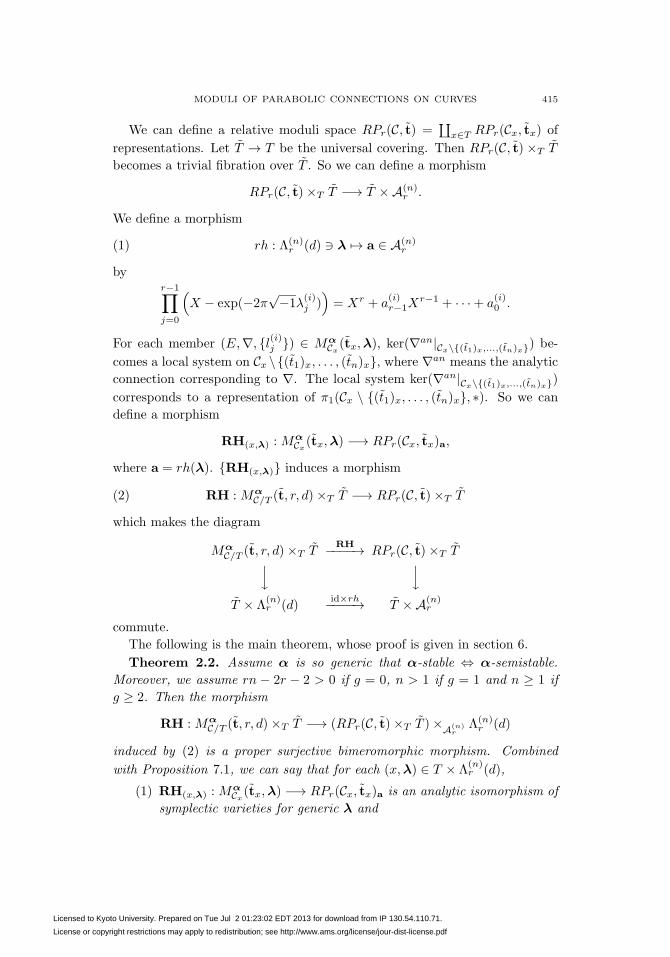
We can define a relative moduli space RPr(C, t) =∐
x∈T RPr(Cx, tx) of
representations. Let T → T be the universal covering. Then RPr(C, t)×T T
becomes a trivial fibration over T . So we can define a morphism
RPr(C, t)×T T −→ T ×A(n)r .
We define a morphism
(1) rh : Λ(n)r (d) � λ �→ a ∈ A(n)
r
byr−1∏j=0
(X − exp(−2π
√−1λ
(i)j ))= Xr + a
(i)r−1X
r−1 + · · ·+ a(i)0 .
For each member (E,∇, {l(i)j }) ∈ MαCx(tx,λ), ker(∇an|Cx\{(t1)x,...,(tn)x}) be-
comes a local system on Cx \{(t1)x, . . . , (tn)x}, where ∇an means the analytic
connection corresponding to ∇. The local system ker(∇an|Cx\{(t1)x,...,(tn)x})
corresponds to a representation of π1(Cx \ {(t1)x, . . . , (tn)x}, ∗). So we can
define a morphism
RH(x,λ) : MαCx(tx,λ) −→ RPr(Cx, tx)a,
where a = rh(λ). {RH(x,λ)} induces a morphism
(2) RH : MαC/T (t, r, d)×T T −→ RPr(C, t)×T T
which makes the diagram
MαC/T (t, r, d)×T T
RH−−−−→ RPr(C, t)×T T⏐⏐� ⏐⏐�T × Λ
(n)r (d)
id×rh−−−−→ T ×A(n)r
commute.
The following is the main theorem, whose proof is given in section 6.
Theorem 2.2. Assume α is so generic that α-stable ⇔ α-semistable.
Moreover, we assume rn − 2r − 2 > 0 if g = 0, n > 1 if g = 1 and n ≥ 1 if
g ≥ 2. Then the morphism
RH : MαC/T (t, r, d)×T T −→ (RPr(C, t)×T T )×A(n)
rΛ(n)r (d)
induced by (2) is a proper surjective bimeromorphic morphism. Combined
with Proposition 7.1, we can say that for each (x,λ) ∈ T × Λ(n)r (d),
(1) RH(x,λ) : MαCx(tx,λ) −→ RPr(Cx, tx)a is an analytic isomorphism of
symplectic varieties for generic λ and
Licensed to Kyoto University. Prepared on Tue Jul 2 01:23:02 EDT 2013 for download from IP 130.54.110.71.
License or copyright restrictions may apply to redistribution; see http://www.ams.org/license/jour-dist-license.pdf
416 MICHI-AKI INABA
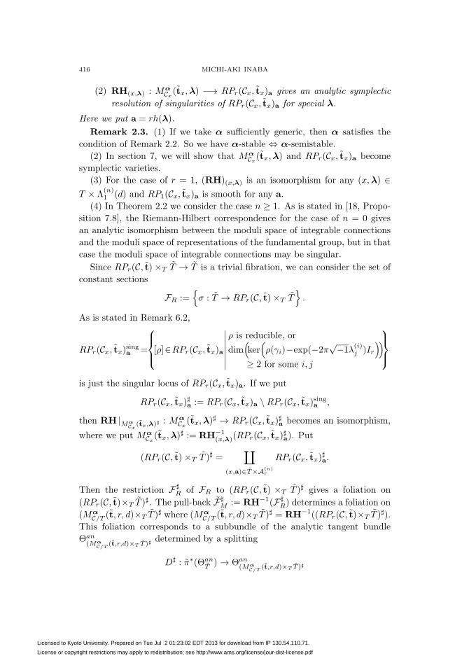
(2) RH(x,λ) : MαCx(tx,λ) −→ RPr(Cx, tx)a gives an analytic symplectic
resolution of singularities of RPr(Cx, tx)a for special λ.
Here we put a = rh(λ).
Remark 2.3. (1) If we take α sufficiently generic, then α satisfies the
condition of Remark 2.2. So we have α-stable ⇔ α-semistable.
(2) In section 7, we will show that MαCx(tx,λ) and RPr(Cx, tx)a become
symplectic varieties.
(3) For the case of r = 1, (RH)(x,λ) is an isomorphism for any (x,λ) ∈T × Λ
(n)1 (d) and RP1(Cx, tx)a is smooth for any a.
(4) In Theorem 2.2 we consider the case n ≥ 1. As is stated in [18, Propo-
sition 7.8], the Riemann-Hilbert correspondence for the case of n = 0 gives
an analytic isomorphism between the moduli space of integrable connections
and the moduli space of representations of the fundamental group, but in that
case the moduli space of integrable connections may be singular.
Since RPr(C, t)×T T → T is a trivial fibration, we can consider the set of
constant sections
FR :={σ : T → RPr(C, t)×T T
}.
As is stated in Remark 6.2,
RPr(Cx, tx)singa =
⎧⎪⎨⎪⎩[ρ]∈RPr(Cx, tx)a
∣∣∣∣∣∣∣ρ is reducible, or
dim(ker(ρ(γi)−exp(−2π
√−1λ
(i)j )Ir
))≥ 2 for some i, j
⎫⎪⎬⎪⎭
is just the singular locus of RPr(Cx, tx)a. If we put
RPr(Cx, tx)�a := RPr(Cx, tx)a \RPr(Cx, tx)singa ,
then RH |MαCx
(tx,λ)� : MαCx(tx,λ)
� → RPr(Cx, tx)�a becomes an isomorphism,
where we put MαCx(tx,λ)
� := RH−1(x,λ)(RPr(Cx, tx)�a). Put
(RPr(C, t)×T T )� =∐
(x,a)∈T×A(n)r
RPr(Cx, tx)�a.
Then the restriction F�R of FR to (RPr(C, t) ×T T )� gives a foliation on
(RPr(C, t)×T T )�. The pull-back F�
M := RH−1(F�R) determines a foliation on
(MαC/T (t, r, d)×T T )
� where (MαC/T (t, r, d)×T T )
� = RH−1((RPr(C, t)×T T )�).
This foliation corresponds to a subbundle of the analytic tangent bundle
Θan(Mα
C/T(t,r,d)×T T )�
determined by a splitting
D� : π∗(ΘanT) → Θan
(MαC/T
(t,r,d)×T T )�
Licensed to Kyoto University. Prepared on Tue Jul 2 01:23:02 EDT 2013 for download from IP 130.54.110.71.
License or copyright restrictions may apply to redistribution; see http://www.ams.org/license/jour-dist-license.pdf
MODULI OF PARABOLIC CONNECTIONS ON CURVES 417
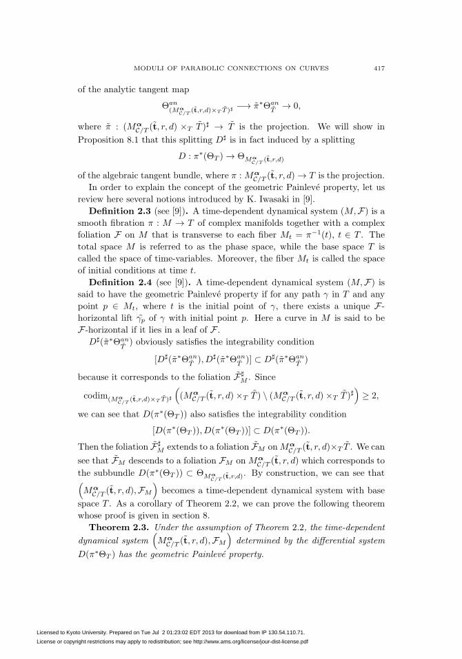
of the analytic tangent map
Θan(Mα
C/T(t,r,d)×T T )�
−→ π∗ΘanT
→ 0,
where π : (MαC/T (t, r, d) ×T T )� → T is the projection. We will show in
Proposition 8.1 that this splitting D� is in fact induced by a splitting
D : π∗(ΘT ) → ΘMαC/T
(t,r,d)
of the algebraic tangent bundle, where π : MαC/T (t, r, d) → T is the projection.
In order to explain the concept of the geometric Painleve property, let us
review here several notions introduced by K. Iwasaki in [9].
Definition 2.3 (see [9]). A time-dependent dynamical system (M,F) is a
smooth fibration π : M → T of complex manifolds together with a complex
foliation F on M that is transverse to each fiber Mt = π−1(t), t ∈ T . The
total space M is referred to as the phase space, while the base space T is
called the space of time-variables. Moreover, the fiber Mt is called the space
of initial conditions at time t.
Definition 2.4 (see [9]). A time-dependent dynamical system (M,F) is
said to have the geometric Painleve property if for any path γ in T and any
point p ∈ Mt, where t is the initial point of γ, there exists a unique F-
horizontal lift γp of γ with initial point p. Here a curve in M is said to be
F-horizontal if it lies in a leaf of F .
D�(π∗ΘanT) obviously satisfies the integrability condition
[D�(π∗ΘanT), D�(π∗Θan
T)] ⊂ D�(π∗Θan
T)
because it corresponds to the foliation F�M . Since
codim(MαC/T
(t,r,d)×T T )�
((Mα
C/T (t, r, d)×T T ) \ (MαC/T (t, r, d)×T T )�
)≥ 2,
we can see that D(π∗(ΘT )) also satisfies the integrability condition
[D(π∗(ΘT )), D(π∗(ΘT ))] ⊂ D(π∗(ΘT )).
Then the foliation F�M extends to a foliation FM onMα
C/T (t, r, d)×T T . We can
see that FM descends to a foliation FM on MαC/T (t, r, d) which corresponds to
the subbundle D(π∗(ΘT )) ⊂ ΘMαC/T
(t,r,d). By construction, we can see that(Mα
C/T (t, r, d),FM
)becomes a time-dependent dynamical system with base
space T . As a corollary of Theorem 2.2, we can prove the following theorem
whose proof is given in section 8.
Theorem 2.3. Under the assumption of Theorem 2.2, the time-dependent
dynamical system(Mα
C/T (t, r, d),FM
)determined by the differential system
D(π∗ΘT ) has the geometric Painleve property.
Licensed to Kyoto University. Prepared on Tue Jul 2 01:23:02 EDT 2013 for download from IP 130.54.110.71.
License or copyright restrictions may apply to redistribution; see http://www.ams.org/license/jour-dist-license.pdf
418 MICHI-AKI INABA
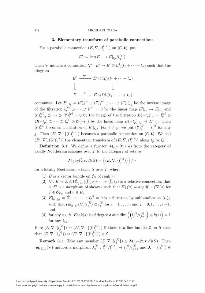
3. Elementary transform of parabolic connections
For a parabolic connection (E,∇, {l(i)j }) on (C, t), put
E′ := ker(E −→ E|tp/l(p)q ).
Then ∇ induces a connection ∇′ : E′ → E′ ⊗Ω1C(t1 + · · ·+ tn) such that the
diagram
E′ ∇′−−−−→ E′ ⊗ Ω1
C(t1 + · · ·+ tn)⏐⏐� ⏐⏐�E
∇−−−−→ E ⊗ Ω1C(t1 + · · ·+ tn)
commutes. Let E′|tp = (l′)(p)0 ⊃ (l′)
(p)1 ⊃ · · · ⊃ (l′)
(p)r−q be the inverse image
of the filtration l(p)q ⊃ · · · ⊃ l
(p)r = 0 by the linear map E′|tp → E|tp and
(l′)(p)r−q ⊃ · · · ⊃ (l′)
(p)r = 0 be the image of the filtration E(−tp)|tp = l
(p)0 ⊗
O(−tp) ⊃ · · · ⊃ l(p)q ⊗ O(−tp) by the linear map E(−tp)|tp → E′|tp . Then
(l′)(p)∗ becomes a filtration of E′|tp . For i �= p, we put (l′)
(i)j = l
(i)j for any
j. Then (E′,∇′, {(l′)(i)j }) becomes a parabolic connection on (C, t). We call
(E′,∇′, {(l′)(i)j }) the elementary transform of (E,∇, {l(i)j }) along tp by l(p)q .
Definition 3.1. We define a functor MC/T (t, r, d) from the category of
locally Noetherian schemes over T to the category of sets by
MC/T (t, r, d)(S) ={(E,∇, {l(i)j })
}/ ∼
for a locally Noetherian scheme S over T , where
(1) E is a vector bundle on CS of rank r,
(2) ∇ : E → E ⊗Ω1CS/S
((t1)S + · · ·+ (tn)S) is a relative connection, that
is, ∇ is a morphism of sheaves such that ∇(fa) = a⊗ df + f∇(a) for
f ∈ OCSand a ∈ E,
(3) E|(ti)S = l(i)0 ⊃ · · · ⊃ l
(i)r = 0 is a filtration by subbundles on (ti)S
such that res(ti)S (∇)(l(i)j ) ⊂ l
(i)j for i = 1, . . . , n and j = 0, 1, . . . , r−1,
and
(4) for any s ∈ S, E⊗k(s) is of degree d and dim((
l(i)j /l
(i)j+1
)⊗ k(s)
)= 1
for any i, j.
Here (E,∇, {l(i)j }) ∼ (E′,∇′, {(l′)(i)j }) if there is a line bundle L on S such
that (E,∇, {l(i)j }) ∼= (E′,∇′, {(l′)(i)j })⊗ L.Remark 3.1. Take any member (E,∇, {l(i)j }) ∈ MC/T (t, r, d)(S). Then
res(ti)S (∇) induces a morphism λ(i)j : l
(i)j /l
(i)j+1 → l
(i)j /l
(i)j+1 and λ = (λ
(i)j ) ∈
Licensed to Kyoto University. Prepared on Tue Jul 2 01:23:02 EDT 2013 for download from IP 130.54.110.71.
License or copyright restrictions may apply to redistribution; see http://www.ams.org/license/jour-dist-license.pdf
MODULI OF PARABOLIC CONNECTIONS ON CURVES 419
Λ(n)r (d)(S). So we obtain a canonical morphism
λ : MC/T (t, r, d) −→ hΛ
(n)r (d)
.
Since there is a canonical morphism MC/T (t, r, d) → hT , we obtain a mor-
phism
(x, λ) : MC/T (t, r, d) −→ hT × hΛ
(n)r (d)
= hT×Λ
(n)r (d)
.
Definition 3.2. For C-valued points λ ∈ Λ(n)r (d)(C), x ∈ T (C), (x,λ)
can be considered as a morphism hSpecC → hT × hΛ
(n)r (d)
. Then we put
MCx(tx,λ) = MC/T (t, r, d)×h
T×Λ(n)r (d)
hSpecC.
MCx(tx,λ) can be considered as a functor from the category of locally Noe-
therian schemes over C to the category of sets.
For a locally Noetherian scheme S over T , take any member (E,∇, {l(i)j }) ∈MC/T (t, r, d)(S). For (p, q) with 1 ≤ p ≤ n and 0 ≤ q ≤ r, we put
E′ := ker(E −→ (E|(tp)S/l
(p)q )).
Then ∇ induces a relative connection
∇′ : E′ −→ E′ ⊗ Ω1CS/S((t1)S + · · ·+ (tn)S)
such that the diagram
E′ ∇′−−−−→ E′ ⊗ Ω1
CS/S((t1)S + · · ·+ (tn)S)⏐⏐� ⏐⏐�
E∇−−−−→ E ⊗ Ω1
CS/S((t1)S + · · ·+ (tn)S)
is commutative. Note that the sequence
E(−(tp)S)|(tp)Sπ−→ E′|(tp)S
ι−→ E|(tp)Sis an exact sequence. Im ι = l
(p)q is a subbundle of E|(tp)S and Imπ = ker ι is
a subbundle of E′|(tp)S . Moreover kerπ = l(p)q ⊗OCS
(−(tp)S) is a subbundle
of E(−(tp)S)|(tp)S . Let E′|(tp)S = (l′)(p)0 ⊃ · · · ⊃ (l′)
(p)r−q be the inverse image
by ι : E′|(tp)S → E|(tp)S of the filtration l(p)q ⊃ · · · ⊃ l
(p)r . Then each (l′)
(p)j is
a subbundle of E′|(tp)S for 0 ≤ j ≤ r − q. Let (l′)(p)r−q ⊃ · · · ⊃ (l′)
(p)r be the
image by π : E(−(tp)S)|(tp)S → E′|(tp)S of the filtration l(p)0 ⊗OCS
(−(tp)S) ⊃· · · ⊃ l
(p)q ⊗OCS
(−(tp)S). For each j with 0 ≤ j ≤ q, l(p)j ⊗OCS
(−(tp)S)/l(p)q ⊗
OCS(−(tp)S)
∼→ (l′)(p)r−q+j is a subbundle of E(−(tp)S)|(tp)S/ kerπ ∼= Imπ =
ker ι. So (l′)(p)r−q+j is a subbundle of E′|(tp)S for any j with 0 ≤ j ≤ q.
Licensed to Kyoto University. Prepared on Tue Jul 2 01:23:02 EDT 2013 for download from IP 130.54.110.71.
License or copyright restrictions may apply to redistribution; see http://www.ams.org/license/jour-dist-license.pdf
420 MICHI-AKI INABA
For i �= p with 1 ≤ i ≤ n, we put (l′)(i)j := l
(i)j for 0 ≤ j ≤ r. Then
(E′,∇′, {(l′)(i)j }) becomes a member of MC/T (t, r, d− q)(S). We say (E′,∇′,
{(l′)(i)j }) is the elementary transform of (E,∇, {l(i)j }) along (tp)S by l(p)q . The
elementary transform induces a morphism
Elm(p)q : MC/T (t, r, d) −→ MC/T (t, r, d− q)(3)
(E,∇, {l(i)j }) �→ (E′,∇′, {(l′)(i)j })(4)
of functors. For any member (E,∇, {l(i)j }) ∈ MC/T (t, r, d)(S), we have
Elm(p)r−q ◦ Elm(p)
q (E,∇, {l(i)j })
= Elm(p)r−q(E
′,∇′, {(l′)(i)j })
= (E(−(tp)S),∇|E(−(tp)S), {l(i)j ⊗OCS
(−(tp)S)}).
If we put
bp : MC/T (t, r, d− r)∼−→ MC/T (t, r, d)(5)
(E,∇, {l(i)j }) �→ (E ⊗OC(tp),∇⊗ idOC(tp) + idE ⊗ dOC(tp), {l(i)j ⊗OC(tp)}),
(6)
then we have bp ◦ Elm(p)r−q ◦ Elm(p)
q = idMC/T (t,r,d). We can also check that
Elm(p)q ◦ bp ◦ Elm(p)
r−q = bp ◦ Elm(p)q ◦ Elm(p)
r−q
= idMC/T (t,r,d−q).
Thus Elm(p)q is an isomorphism:
Elm(p)q : MC/T (t, r, d)
∼−→ MC/T (t, r, d− q).
Take any C-valued points x ∈ T (C), λ ∈ Λ(n)r (d)(C). We put
((λ′)(p)0 , . . . , (λ′)
(p)r−1) = (λ(p)
q , λ(p)q+1, . . . , λ
(p)r−1, λ
(p)0 + 1, λ
(p)1 + 1, . . . , λ
(p)q−1 + 1)
and (λ′)(i)j := λ
(i)j for i �= p with 1 ≤ i ≤ n and 0 ≤ j ≤ r − 1. Then
λ′ := ((λ′)(i)j ) ∈ Λ
(n)r (d−q)(C). For a member (E,∇, {l(i)j }) ∈ MCx
(tx,λ)(S),
Elm(p)q (E,∇, {l(i)j }) ∈ MCx
(tx,λ′)(S). So Elm(p)
q induces an isomorphism
(7) Elm(p)q : MCx
(tx,λ)∼−→ MCx
(tx,λ′).
Take a point λ ∈ Λ(n)r (d)(C). We can write
r−1∏j=0
(x− λ(p)j ) =
u∏k=1
(x− μ(p)k )m
(p)k ,
Licensed to Kyoto University. Prepared on Tue Jul 2 01:23:02 EDT 2013 for download from IP 130.54.110.71.
License or copyright restrictions may apply to redistribution; see http://www.ams.org/license/jour-dist-license.pdf
MODULI OF PARABOLIC CONNECTIONS ON CURVES 421
where Re(μ(p)1 ) ≥ Re(μ
(p)2 ) ≥ · · · ≥ Re(μ
(p)u ), Im(μ
(p)j ) > Im(μ
(p)j+1) if
Re(μ(p)j ) = Re(μ
(p)j+1) and x is an indeterminate. For any member (E,∇E,
{l(i)j }) ∈ MCx(tx,λ)(S), we can find j
(k)0 , j
(k)1 , . . . , j
(k)
m(p)k
for 1 ≤ k ≤ u satis-
fying 0 ≤ j(k)0 < j
(k)1 < · · · < j
(k)
m(p)k
≤ r such that
(ker
(res(tp)x(∇E)− μ
(p)k · id
)r
∩ l(p)
j(k)m
)/(ker
(res(tp)x(∇E)− μ
(p)k · id
)r
∩ l(p)
j(k)m+1
)
∼−→ l(p)
j(k)m
/l(p)
j(k)m +1
for m = 0, . . . ,m(p)k − 1. Let E|(tp)x = (l′)
(p)0 ⊃ (l′)
(p)1 ⊃ · · · ⊃ (l′)
(p)r−1 ⊃
(l′)(p)r = 0 be the filtration by subbundles satisfying rank(l′)
(p)j /(l′)
(p)j+1 = 1 for
j = 0, . . . , r − 1 and
(l′)(p)q =(ker(res(tp)x(∇E)− μ
(p)k · id
)r∩ l
(p)
j(k)m
)+ (l′)
(p)q+1
for q = 0, . . . , r− 1, where q = r− (m(p)k −m)−
∑k<k′≤u m
(p)k′ , 1 ≤ k ≤ u and
0 ≤ m < m(p)k . We put
(ν(p)0 , . . . , ν
(p)r−1) := (
m(p)1︷ ︸︸ ︷
μ(p)1 , . . . , μ
(p)1 , . . . ,
m(p)k︷ ︸︸ ︷
μ(p)k , . . . , μ
(p)k , . . . ,
m(p)u︷ ︸︸ ︷
μ(p)u , . . . , μ(p)
u ),
ν(i)j = λ
(i)j for i �= p and ν := (ν
(i)j )i,j . Then the correspondence (E,∇E, {l(i)j })
�→ (E,∇E, {(l′)(i)j }) determines an isomorphism
(8) ap : MCx(tx,λ)
∼−→ MCx(tx,ν)
of functors.
Looking at the change of λ under the transformations Elm(i)j and bi, we
can easily see the following proposition, which is useful in considering the
Riemann-Hilbert correspondence in section 6.
Proposition 3.1. Composing the isomorphisms ai, bi and Elm(i)j for i =
1, . . . , n, j = 1, . . . , r given in (8), (7) and (5), we obtain an isomorphism
(9) σ : MCx(tx,λ)
∼−→ MCx(tx,μ)
of functors, where 0 ≤ Re(μ(i)j ) < 1 for any i, j.
As a corollary, we obtain the following:
Corollary 3.1. Take λ ∈ Λ(n)r (d) and μ ∈ Λ
(n)r (d′) which satisfy rh(λ) =
rh(μ) ∈ A(n)r , where rh is the morphism defined in (1). Then we can obtain
Licensed to Kyoto University. Prepared on Tue Jul 2 01:23:02 EDT 2013 for download from IP 130.54.110.71.
License or copyright restrictions may apply to redistribution; see http://www.ams.org/license/jour-dist-license.pdf
422 MICHI-AKI INABA
by composing ai, a−1i , bi, b
−1i and Elm
(i)j an isomorphism
σ : MCx(tx,λ)
∼−→ MCx(tx,μ)
of functors.
Proof. Applying Proposition 3.1, we obtain an isomorphism
σ : MCx(tx,λ)
∼−→ MCx(tx,ν)
of functors, where 0 ≤ Re(ν(i)j ) < 1 for any i, j. By composing ai, we may also
assume that Re(ν(i)0 ) ≥ Re(ν
(i)1 ) ≥ · · · ≥ Re(ν
(i)r−1) for any i and Im(ν
(i)j ) ≥
Im(ν(i)j+1) if Re(ν
(i)j ) = Re(ν
(i)j+1). Applying Proposition 3.1 again, we have an
isomorphism
σ′ : MCx(tx,μ)
∼−→ MCx(tx,ν).
Then
(σ′)−1 ◦ σ : MCx(tx,λ)
∼−→ MCx(tx,μ)
is the desired isomorphism. �
4. Moduli of stable parabolic connections
Before proving Theorem 2.1, we recall the definition of parabolic Λ1D-triple
defined in [7]. Let D be an effective divisor on a curve C. We define Λ1D as
OC ⊕ Ω1C(D)∨ with the bimodule structure given by
f(a, v) = (fa, fv) (f, a ∈ OC , v ∈ Ω1C(D)∨),
(a, v)f = (fa+ v(f), fv) (f, a ∈ OC , v ∈ Ω1C(D)∨).
Definition 4.1. We say (E1, E2,Φ, F∗(E1)) is a parabolic Λ1D-triple on C
of rank r and degree d if
(1) E1 and E2 are vector bundles on C of rank r and degree d,
(2) Φ : Λ1D ⊗ E1 → E2 is a left OC -homomorphism, and
(3) E1 = F1(E1) ⊃ F2(E1) ⊃ · · · ⊃ Fl(E1) ⊃ Fl+1(E1) = E1(−D) is a
filtration by coherent subsheaves.
Note that to give a left OC-homomorphism Φ : Λ1D⊗E1 → E2 is equivalent
to giving an OC-homomorphism φ : E1 → E2 and a morphism ∇ : E1 → E2⊗Ω1
C(D) such that ∇(fa) = φ(a)⊗df +f∇(a) for f ∈ OC and a ∈ E1. We also
denote the parabolic Λ1D-triple (E1, E2,Φ, F∗(E1)) by (E1, E2, φ,∇, F∗(E1)).
We take positive integers β1, β2, γ and rational numbers 0 < α′1 < · · · <
α′l < 1. We assume γ � 0.
Licensed to Kyoto University. Prepared on Tue Jul 2 01:23:02 EDT 2013 for download from IP 130.54.110.71.
License or copyright restrictions may apply to redistribution; see http://www.ams.org/license/jour-dist-license.pdf
MODULI OF PARABOLIC CONNECTIONS ON CURVES 423
Definition 4.2. A parabolic Λ1D-triple (E1, E2,Φ, F∗(E1)) is (α,β, γ)-
stable (resp. (α,β, γ)-semistable) if for any subbundles (F1, F2) ⊂ (E1, E2)
satisfying (0, 0) �= (F1, F2) �= (E1, E2) and Φ(Λ1D(t)⊗F1) ⊂ F2, the inequality
β1 degF1(−D) + β2(degF2 − γ rankF2) + β1
∑lj=1 α
′j length(
Fj(E1)∩F1
Fj+1(E1)∩F1)
β1 rankF1 + β2 rankF2
<
(resp.≤)
β1 degE1(−D)+β2(degE2−γ rankE2)+β1
∑lj=1 α
′j length(
Fj(E1)Fj+1(E1)
)
β1 rankE1+β2 rankE2
holds.
Theorem 4.1 (see [7], Theorem 5.1). Let S be an algebraic scheme over
C, C be a flat family of smooth projective curves of genus g and D be an
effective Cartier divisor on C flat over S. Then there exists a coarse mod-
uli scheme MD,α′,β,γC/S (r, d, {di}1≤i≤nr) of (α
′,β, γ)-stable parabolic Λ1D-triples
(E1, E2,Φ, F∗(E1)) on C over S such that r = rankE1 = rankE2, d =
degE1 = degE2 and di = length(E1/Fi+1(E1)). If α′ is generic, it is projec-
tive over S.
Definition 4.3. We denote the pull-back of C and t by the morphism
T ×Λ(n)r (d) → T by the same characters C and t = (t1, . . . , tn). Then D(t) :=
t1 + · · · + tn becomes an effective Cartier divisor on C flat over T × Λ(n)r (d).
We also denote by λ the pull-back of the universal family on Λ(n)r (d) by the
morphism T × Λ(n)r (d) → Λ
(n)r (d). We define a functor Mα
C/T (t, r, d) of the
category of locally Noetherian schemes to the category of sets by
MαC/T (t, r, d)(S) :=
{(E,∇, {l(i)j })
}/ ∼,
for a locally Noetherian scheme S over T × Λ(n)r (d), where
(1) E is a vector bundle on CS of rank r,
(2) ∇ : E → E ⊗ Ω1CS/S
(D(t)S) is a relative connection,
(3) E|(ti)S = l(i)0 ⊃ l
(i)1 ⊃ · · · ⊃ l
(i)r−1 ⊃ l
(i)r = 0 is a filtration by subbun-
dles such that (res(ti)S (∇) − (λ(i)j )S)(l
(i)j ) ⊂ l
(i)j+1 for 0 ≤ j ≤ r − 1,
i = 1, . . . , n, and
(4) for any geometric point s ∈ S, dim(l(i)j /l
(i)j+1) ⊗ k(s) = 1 for any i, j
and (E,∇, {l(i)j })⊗ k(s) is α-stable.
Here (E,∇, {l(i)j }) ∼ (E′,∇′, {l′(i)j }) if there exists a line bundle L on S and
an isomorphism σ : E∼→ E′ ⊗ L such that σ|ti(l
(i)j ) = l
′(i)j ⊗ L for any i, j,
Licensed to Kyoto University. Prepared on Tue Jul 2 01:23:02 EDT 2013 for download from IP 130.54.110.71.
License or copyright restrictions may apply to redistribution; see http://www.ams.org/license/jour-dist-license.pdf
424 MICHI-AKI INABA
and the diagram
E∇−−−−→ E ⊗ Ω1
C/T (D(t))
σ
⏐⏐� σ⊗id
⏐⏐�E′ ⊗ L ∇′⊗L−−−−→ E′ ⊗ Ω1
C/T (D(t))⊗ Lcommutes.
Proof of Theorem 2.1. Fix a weight α which determines the stability of
parabolic connections. We take positive integers β1, β2, γ and rational num-
bers 0 < α(i)1 < α
(i)2 < · · · < α
(i)r < 1 satisfying (β1 + β2)α
(i)j = β1α
(i)j for
any i, j. We assume γ � 0. We can take an increasing sequence 0 < α′1 <
· · · < α′nr < 1 such that {α′
i|1 ≤ i ≤ nr} ={α(i)j
∣∣∣ 1 ≤ i ≤ n, 1 ≤ j ≤ r}.
Take any member (E,∇, {l(i)j }) ∈ MαC/T (t, r, d)(S). For each 1 ≤ p ≤ rn,
there exists i, j satisfying α(i)j = α′
p. We put F1(E) := E and define in-
ductively Fp+1(E) := ker(Fp(E) → E|(ti)S/l(i)j ) for p = 1, . . . , rn. We also
put dp := length((E/Fp+1(E)) ⊗ k(s)) for p = 1, . . . , rn and s ∈ S. Then
(E,∇, {l(i)j }) �→ (E,E, idE ,∇, F∗(E)) determines a morphism
ι : MαC/T (t, r, d) → MD(t),α′,β,γ
C/T×Λ(n)r (d)
(r, d, {di}1≤i≤nr),
where MD(t),α′,β,γC/T (r, d, {di}1≤i≤nr) is the moduli functor of (α′,β, γ)-stable
parabolic Λ1D(t)
-triples whose coarse moduli scheme exists by Theorem 4.1.
Note that a parabolic connection (E,∇, {l(i)j }) is α-stable if and only if the
corresponding parabolic Λ1D(t)-triple (E,E, id,∇, F∗(E)) is (α′,β, γ)-stable
since γ � 0. We can see that ι is representable by an immersion. So we
can prove in the same way as [7, Theorem 2.1] that a certain subscheme
MαC/T (t, r, d) of M
D(t),α′,β,γC (r, d, {di}1≤i≤nr) is just the coarse moduli scheme
of MαC/T (t, r, d).
Applying a certain elementary transformation, we obtain an isomorphism
σ : MC/T (t, r, d)∼−→ MC/T (t, r, d
′)
of functors, where d′ and r are coprime. Then σ(MαC/T (t, r, d)) can be consid-
ered as the moduli scheme of parabolic connections of rank r and degree d′
satisfying a certain stability condition. We can take a vector space V such that
there exists a surjection V ⊗OCs(−m) → E such that V ⊗ k(s) → H0(E(m))
is isomorphic and hi(E(m)) = 0 for i > 0 for any member (E,∇, {l(i)j }) ∈σ(Mα
C/T (t, r, d)) over s ∈ T . We put P (n) := χ(E(n)). Let E be the universal
family on C ×T×Λ
(n)r (d)
QuotPV⊗OC(−m)/C/T×Λ
(n)r (d)
. Then we can construct
Licensed to Kyoto University. Prepared on Tue Jul 2 01:23:02 EDT 2013 for download from IP 130.54.110.71.
License or copyright restrictions may apply to redistribution; see http://www.ams.org/license/jour-dist-license.pdf
MODULI OF PARABOLIC CONNECTIONS ON CURVES 425
a scheme R over QuotPV⊗OC(−m)/C/T×Λ
(n)r (d)
which parametrizes connections
∇ : Es → Es ⊗ Ω1Cs(D(ts)) and parabolic structures Es|(ti)s = l
(i)0 ⊃ · · · ⊃
l(i)r−1 ⊃ l
(i)r = 0 such that (res(ti)s(∇) − (λ
(i)j )s)(l
(i)j ) ⊂ l
(i)j+1 for any i, j. Then
PGL(V ) canonically acts on R and for some open subscheme Rs of R, there
is a canonical morphism Rs → σ(MαC/T (t, r, d)) which becomes a principal
PGL(V )-bundle. So we can prove in the same manner as [6, Theorem 4.6.5]
that for a certain line bundle L on Rs, E ⊗ L descends to a vector bundle on
C ×T×Λ
(n)r (d)
σ(MαC/T (t, r, d)), since r and d′ are coprime. We can easily see
that the universal families ∇, {l(i)j } of connections and parabolic structures
on E ⊗ L also descend. So we obtain a universal family for the moduli space
σ(MαC/T (t, r, d)), and Mα
C/T (t, r, d) in fact becomes a fine moduli scheme.
Let (E, ∇, {l(i)j }) be a universal family on C ×T MαC/T (t, r, d). We define a
complex F• by
F0 :={s∈End(E)
∣∣∣s|ti×MαC/T
(t,r,d)(l(i)j ) ⊂ l
(i)j for any i, j
},
F1 :={s∈End(E)⊗Ω1
C/T (D(t))∣∣∣resti×Mα
C/T(t,r,d)(s)(l
(i)j )⊂ l
(i)j+1 for any i, j
},
∇F• : F0 −→ F1; ∇F•(s) = ∇ ◦ s− s ◦ ∇.
Let (A,m) be an Artinian local ring over T × Λ(n)r (d), I an ideal of A sat-
isfying mI = 0. Take any member (E,∇, {l(i)j }) ∈ MαC/T (t, r, d)(A/I). We
denote the image of SpecA/m → MαC/T (t, r, d) by x. The structure mor-
phism SpecA → T × Λ(n)r (d) corresponds to an A-valued point (t,λ) ∈
T (A) ×(Λ(n)r (d)
)(A). Let C × SpecA =
⋃α Uα be an affine open cov-
ering such that E|Uα⊗A/I∼= O⊕r
Uα⊗A/I , �{i|ti ∈ Uα} ≤ 1 for any α and
�{α|ti ∈ Uα} ≤ 1 for any i. We can obviously take a vector bundle Eα on Uα
such that there is an isomorphism Eα ⊗ A/Iφα−−→∼
E|Uα⊗A/I . If ti ∈ Uα,
we take a basis e1, e2, . . . , er of Eα such that l(i)r−1 = 〈e1|ti⊗A/I〉, l(i)r−2 =
〈e1|ti⊗A/I , e2|ti⊗A/I〉, . . . , l(i)1 = 〈e1|ti⊗A/I , . . . , er−1|ti⊗A/I〉. The connection
matrix of ∇|E|Uα⊗A/Iwith respect to the basis e1 ⊗A/I, . . . , er ⊗A/I can be
given by a matrix Ωα ∈ Mr(Ω1CA/I/(A/I)((ti)A/I)|Uα⊗A/I) such that
Ωα|ti⊗A/I =
⎛⎜⎜⎜⎜⎝λ(i)r−1 ⊗A/I ω12 · · · ω1r
0 λ(i)r−2 ⊗A/I · · · ω2r
......
. . ....
0 0 · · · λ(i)0 ⊗A/I
⎞⎟⎟⎟⎟⎠ .
Licensed to Kyoto University. Prepared on Tue Jul 2 01:23:02 EDT 2013 for download from IP 130.54.110.71.
License or copyright restrictions may apply to redistribution; see http://www.ams.org/license/jour-dist-license.pdf
426 MICHI-AKI INABA
We can take a lift Ωα ∈ Mr(Ω1CA/A(ti)|Uα
) of Ωα such that
Ωα|ti :=
⎛⎜⎜⎜⎜⎝λ(i)r−1 ω12 · · · ω1r
0 λ(i)r−2 · · · ω2r
......
. . ....
0 0 · · · λ(i)0
⎞⎟⎟⎟⎟⎠ ,
which induces a connection ∇α : Eα → Eα⊗Ω1CA/A((t1+ t2+ · · ·+ tn)A). We
define a parabolic structure {(lα)(i)j } on Eα by (lα)(i)r−1 := 〈e1|ti〉, (lα)
(i)r−2 :=
〈e1|ti , e2|ti〉, . . . , (lα)(i)1 := 〈e1|ti , . . . , er−1|ti〉. Then (Eα,∇α, {(lα)(i)j }) be-
come a lift (E,∇, {l(i)j })|Uα. If ti /∈ Uα, we can easily take a lift (Eα,∇α,
{(lα)(i)j }) of (E,∇, {l(i)j })|Uα. We put Uαβ := Uα ∩ Uβ and Uαβγ := Uα ∩
Uβ ∩ Uγ . Take a lift θβα : Eα|Uαβ
∼→ Eβ|Uαβof the canonical isomorphism
Eα|Uαβ⊗A/I
φα−−→∼
E|Uαβ⊗A/I
φ−1β−−→∼
Eβ|Uαβ⊗A/I. We put
uαβγ : = φα|Uαβγ◦(θ−1γα |Uαβγ
◦ θγβ|Uαβγ◦ θβα|Uαβγ
− idEα|Uαβγ
)◦ φ−1
α |Uαβγ,
vαβ : = φα ◦(∇α|Uαβ
− θ−1βα ◦ ∇β ◦ θβα
)◦ φ−1
α |Uαβγ.
Then we have {uαβγ} ∈ C2({Uα},F0⊗I) and {vαβ} ∈ C1({Uα},F1⊗I). We
can easily see that
d{vαβ} = −∇F•{uαβγ} and d{uαβγ} = 0.
So we can define an element
ω(E,∇, {l(i)j }) := [({uαβγ}, {vαβ})] ∈ H2({Uα},F•⊗I) = H2(F•⊗k(x))⊗I.
We can easily see that (E,∇, {l(i)j }) can be lifted to an A-valued point of
MαC/T (t, r, d) if and only if ω(E,∇, {l(i)j }) = 0 in the hypercohomology
H2(F• ⊗ k(x))⊗ I.
Consider the homomorphism
Tr : H2(F• ⊗ k(x))⊗ I −→ H2(Ω•Cx)⊗ I
[{u′αβγ}, {v′αβ}] �→ [{Tr(u′
αβγ)}, {Tr(v′αβ)}].
Then we can see that Tr(ω(E,∇, {l(i)j })) is just the obstruction class for lift-
ing (detE,∧r ∇) to a pair of a line bundle and a connection with the fixed
residue det(λA) over A. Here det(λA) = (∑r−1
j=0(λ(i)j )A)
1≤i≤n. Since PicdC/T is
smooth over T , there is a line bundle L on CA such that L⊗A/I ∼= det(E). We
can construct a connection ∇0 : L → L ⊗ Ω1CA/A(t1 + · · · + tn) because
H1(End(L) ⊗ Ω1CA/A((t1 + · · · + tn)A)) = 0. We can find a member u ∈
Licensed to Kyoto University. Prepared on Tue Jul 2 01:23:02 EDT 2013 for download from IP 130.54.110.71.
License or copyright restrictions may apply to redistribution; see http://www.ams.org/license/jour-dist-license.pdf
MODULI OF PARABOLIC CONNECTIONS ON CURVES 427
H0(End(L) ⊗ Ω1CA/A((t1 + · · · + tn)A)) such that u ⊗ A/I = ∇0 ⊗ A/I −∧r ∇. Then (L, ∇0 − u) becomes a lift of (det(E),
∧r ∇). If we put μ(i) :=
resti⊗A(∇0−u)−∑
j(λ(i)j )A, then we have μ(i) ∈ I for any i and
∑ni=1 μ
(i) = 0.
Note that there is an exact sequence
H0(I ⊗ End(L)⊗ Ω1CA/A((t1 + · · ·+ tn)A))
−→n⊕
i=1
I ⊗ End(L)⊗ Ω1CA/A((t1 + · · ·+ tn)A)|(ti)A ∼=
n⊕i=1
I
f−→ I ∼= H1(I ⊗ End(L)⊗ Ω1CA/A) −→ 0,
where f is given by f((νi)1≤i≤n) =∑n
i=1 νi. Then we can find an element
ω ∈ I ⊗ H0(End(L) ⊗ Ω1CA/A((t1 + · · · + tn)A)) such that resti⊗A(ω) = μ(i)
for any i. Then (L, ∇0 − u − ω) is a lift of (det(E),∧r ∇) with the residue
(det(λ)A). Thus we have Tr(ω(E,∇, {l(i)j })) = 0. Since (F1)∨ ⊗Ω1CA/A
∼= F0
and (F0)∨ ⊗ Ω1CA/A
∼= F1, we have
H2(F• ⊗ k(x))
∼= coker(H1(F0 ⊗ k(x)) → H1(F1 ⊗ k(x))
)∼= ker
(H0((F1)∨⊗Ω1
C/T ⊗k(x))→H0((F0)∨⊗Ω1C/T ⊗k(x))
)∨∼= ker
(H0(F0 ⊗ k(x)) → H0(F1 ⊗ k(x))
)∨and a commutative diagram
H2(F• ⊗ k(x))Tr−−−−−→ H2(Ω•
Cx)⏐⏐�∼=
⏐⏐�∼=
ker
(H0(F0 ⊗ k(x))
∇F•−→ H0(F1 ⊗ k(x))
)∨ι∨−−−−−→ ker
(H0(OCx)
d→ H0(Ω1Cx
))∨
.
We can see by the stability that the endomorphisms of (E, ∇, {l(i)j })⊗k(x) are
scalar multiplications. So we have ker(H0(F0 ⊗ k(x)) → H0(F1 ⊗ k(x))
)=
k(x) and the canonical inclusion
ι : ker(H0(OCx
)d→ H0(Ω1
Cx))−→ ker
(H0(F0 ⊗ k(x))
∇F•−→ H0(F1 ⊗ k(x)))
is an isomorphism. Hence Tr is an isomorphism and ω(E,∇, {l(i)j }) = 0
because Tr(ω(E,∇, {l(i)j })) = 0. So we have proved that MαC/T (t, r, d) is
smooth over T × Λ(n)r (d).
Take an affine open set M ⊂ MαC/T (t, r, d) and an affine open covering
CM =⋃
α Uα such that E|Uα∼= O⊕r
Uαfor any α, �{i| ti|M ∩ Uα �= ∅} ≤ 1
Licensed to Kyoto University. Prepared on Tue Jul 2 01:23:02 EDT 2013 for download from IP 130.54.110.71.
License or copyright restrictions may apply to redistribution; see http://www.ams.org/license/jour-dist-license.pdf
428 MICHI-AKI INABA
for any α and �{α| ti|M ∩ Uα �= ∅} ≤ 1 for any i. Take a relative tan-
gent vector field v ∈ ΘMα
C/T(t,r,d)/T×Λ
(n)r (d)
(M). v corresponds to a member
(Eε,∇ε, {(lε)(i)j }) ∈ MαC/T (t, r, d)(SpecOM [ε]) such that (Eε,∇ε, {(lε)(i)j }) ⊗
OM [ε]/(ε) ∼= (E, ∇, {l(i)j })|CM, where OM [ε] = OM [t]/(t2). There is an iso-
morphism
ϕα : Eε|Uα×SpecOM [ε]∼→ O⊕r
Uα×SpecOM [ε]
∼→ E|Uα⊗OM [ε]
such that ϕα ⊗ OM [ε]/(ε) : Eε ⊗ OM [ε]/(ε)|Uα
∼→ E|Uα⊗ OM [ε]/(ε) = E|Uα
is the given isomorphism and that ϕα|ti⊗OM [ε]((lε)(i)j ) = l
(i)j |Uα×SpecOM [ε] if
ti|M ∩ Uα �= ∅. We put
uαβ := ϕα ◦ ϕ−1β − idE|Uαβ⊗OM [ε]
,
vα := (ϕα ⊗ id) ◦ ∇ε|Uα⊗OM [ε] ◦ ϕ−1α − ∇|Uα⊗OM [ε].
Then {uαβ} ∈ C1((ε)⊗F0M ), {vα} ∈ C0((ε)⊗F1
M ) and
d{uαβ} = {uβγ − uαγ + uαβ} = 0, ∇F•{uαβ} = {vβ − vα} = d{vα}.
So [({uαβ}, {vα})] determines an element σM (v) of H1(F•M ). We can check
that v �→ σ(v) determines an isomorphism
σM : ΘMα
C/T(t,r,d)/T×Λ
(n)r (d)
(M)∼−→ H1(F•
M ).
These isomorphisms σM induce a canonical isomorphism
σ : ΘMα
C/T(t,r,d)/T×Λ
(n)r (d)
∼−→ R1(πT×Λ
(n)r (d)
)∗(F•),
where πT×Λ
(n)r (d)
: C → T × Λ(n)r (d) is the projection. From the hypercoho-
mology spectral sequence Hq(Fp ⊗ k(x)) ⇒ Hp+q(F• ⊗ k(x)), we obtain an
exact sequence
0 → k(x) → H0(F0(x)) → H0(F1(x)) → H1(F•(x)) → H1(F0(x))
→ H1(F1(x)) → k(x) → 0
for any x ∈ MαC/T (t, r, d). Here we denote F0⊗k(x) by F0(x) and so on. So we
have dimH1(F•(x)) = −2χ(F0(x)) + 2, because H0(F1(x)) ∼= H1(F0(x))∨
and H1(F1(x)) ∼= H0(F0(x))∨. We define E1 by the exact sequence
0 −→ E1 −→ End(E(x)) −→n⊕
i=1
Hom(l(i)1 (x),
(l(i)0 /l
(i)1
)(x))−→ 0.
Inductively we define Ek by the exact sequence
0 −→ Ek −→ Ek−1 −→n⊕
i=1
Hom(l(i)k (x),
(l(i)k−1/l
(i)k
)(x))−→ 0.
Licensed to Kyoto University. Prepared on Tue Jul 2 01:23:02 EDT 2013 for download from IP 130.54.110.71.
License or copyright restrictions may apply to redistribution; see http://www.ams.org/license/jour-dist-license.pdf
MODULI OF PARABOLIC CONNECTIONS ON CURVES 429
Then we have Er−1 = F0(x). So we have
χ(F0(x)) = χ(End(E(x)))− nr(r − 1)/2 = r2(1− g)− nr(r − 1)/2.
Thus we can see that every fiber of MαC/T (t, r, d) over T × Λ
(n)r (d) is equi-
dimensional and its dimension is 2r2(g − 1) + nr(r − 1) + 2 if it is non-
empty. �Proposition 4.1. Let (E,∇E, {l(i)j }) ∈ MC/T (t, r, d)(S) be a flat family
of parabolic connections over a Noetherian scheme S over C. Then the subset
Us := {s ∈ S|(E,∇E, {l(i)j })⊗ k(s) is α-stable}
is a Zariski open subset of S. Take a flat family (E,∇E, {l(i)j }) ∈ MC(t,λ)(S)
of (t,λ)-parabolic connections over a Noetherian scheme S over C. Then
U irr := {s ∈ S|(E,∇E, {l(i)j })⊗ k(s) is irreducible}
is a Zariski open subset of S. Note that a parabolic connection (E,∇E, {l(i)j })is reducible if there is a subbundle 0 �= F � E such that ∇E(F ) ⊂ F ⊗Ω1
C(t1 + . . .+ tn). A parabolic connection (E,∇E, {l(i)j }) is irreducible if it is
not reducible.
Proof. Take (E,∇E, {l(i)j }) ∈ M(t, r, d)(S). As in the proof of Theorem
2.1, a member of (E,E, id,∇, F∗(E)) ∈ MD(t)
C/T×Λ(n)r (d)
(r, d, {di}1≤i≤nr)(S),
where MD(t)
C/T×Λ(n)r (d)
(r, d, {di}1≤i≤nr) is the moduli functor of parabolic
Λ1D(t)/T
-triples without stability condition. By [7, Proposition 5.3],
Ss = {s ∈ S|(E,E, id,∇, F∗(E))⊗ k(s) is (α′, β, γ)-stable}
is a Zariski open subset of S. As in the proof of Theorem 2.1, (E,∇, {l(i)j })⊗k(s) is α-stable if and only if the corresponding parabolic Λ1
D(t)s-triple is
(α′, β, γ)-stable. So we have Ss = Us.
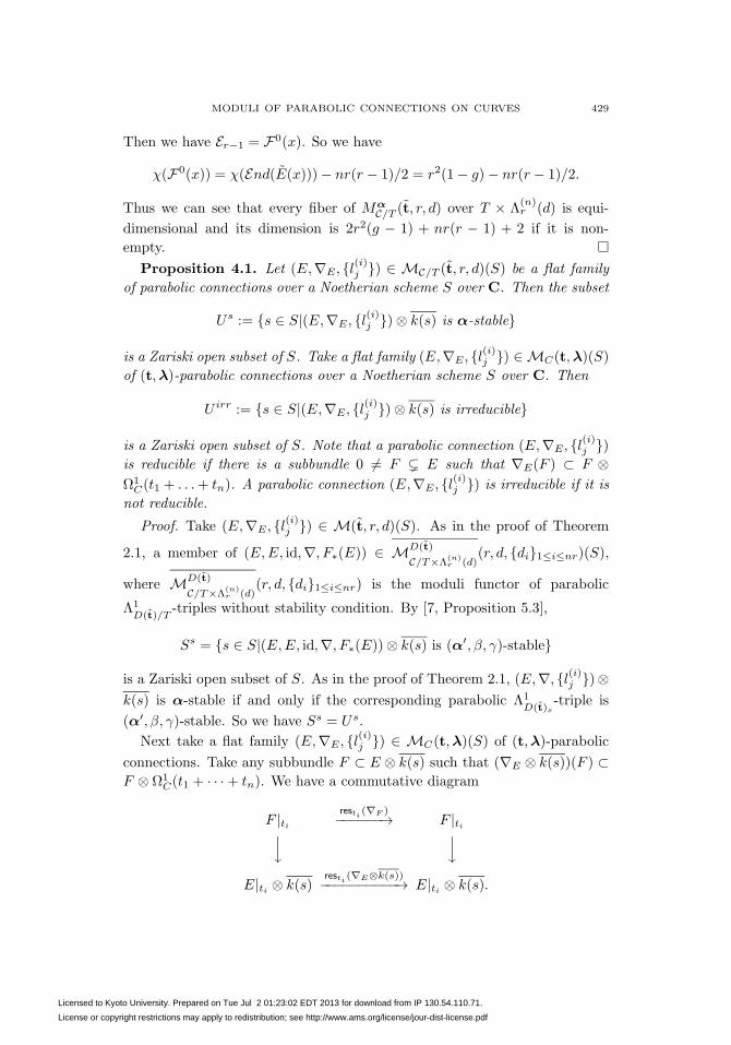
Next take a flat family (E,∇E, {l(i)j }) ∈ MC(t,λ)(S) of (t,λ)-parabolic
connections. Take any subbundle F ⊂ E ⊗ k(s) such that (∇E ⊗ k(s))(F ) ⊂F ⊗ Ω1
C(t1 + · · ·+ tn). We have a commutative diagram
F |tiresti (∇F )−−−−−−→ F |ti⏐⏐� ⏐⏐�
E|ti ⊗ k(s)resti (∇E⊗k(s))−−−−−−−−−−→ E|ti ⊗ k(s).
Licensed to Kyoto University. Prepared on Tue Jul 2 01:23:02 EDT 2013 for download from IP 130.54.110.71.
License or copyright restrictions may apply to redistribution; see http://www.ams.org/license/jour-dist-license.pdf
430 MICHI-AKI INABA
Then we can see that the eigenvalues {μ(i)j } of resti(∇F ) are eigenvalues of
resti(∇E ⊗ k(s)). So the set
P :=
⎧⎨⎩(rank(F ), deg(F ))
∣∣∣∣∣∣F is a non-zero proper subbundle
of E ⊗ k(s) such that
(∇E ⊗ k(s))(F ) ⊂ F ⊗ Ω1C(t1 + · · ·+ tn)
⎫⎬⎭
is finite, because deg(F ) = −∑
i,j μ(i)j . For (r′, d′) ∈ P, put P(r′,d′)(m) =
r′(m − g + 1) + d′ which is a polynomial in m. Then consider the Quot-
scheme Q(r′,d′) := Quotχ(E(m)⊗k(s))−P(r′,d′)(m)
E/C/C and let F (r′,d′) ⊂ EQ(r′,d′) be
the universal subsheaf. Let Y(r′,d′) be the maximal closed subscheme ofQ(r′,d′)
such that the composite
F (r′,d′)Y(r′,d′)
↪→ EY(r′,d′)
(∇E)Y(r′,d′)−−−−−−−−→ EY(r′,d′)
⊗ Ω1C(t1 + · · ·+ tn) −→ (EY(r′,d′)/F
(r′,d′)Y(r′,d′)
)⊗ Ω1C(t1 + · · ·+ tn)
is zero. Since the structure morphism f(r′,d′) : Y(r′,d′) → S is proper,
U irr = S \⋃
(r′,d′)∈Pf(r′,d′)(Y(r′,d′))
is a Zariski open subset of S. �Proposition 4.2. The set
RPr(C, t)irr = {[ρ] ∈ RPr(C, t)|ρ is an irreducible representation}
is a Zariski open subset of RPr(C, t).
Proof. Note that for the quotient morphism
p : Hom(π1(C \ {t1, . . . , tn}, ∗), GLr(C)) −→ RPr(C, t),
Z ⊂ RPr(C, t) is a Zariski closed subset if and only if p−1(Z) is a Zariski
closed subset of Hom(π1(C \ {t1, . . . , tn}, ∗), GLr(C)). There is a universal
representation ρ given by
ρ(αi) : O⊕rHom(π1(C\{t1,...,tn},∗),GLr(C))
∼−→ O⊕rHom(π1(C\{t1,...,tn},∗),GLr(C))
ρ(βi) : O⊕rHom(π1(C\{t1,...,tn},∗),GLr(C))
∼−→ O⊕rHom(π1(C\{t1,...,tn},∗),GLr(C))
ρ(γj) : O⊕rHom(π1(C\{t1,...,tn},∗),GLr(C))
∼−→ O⊕rHom(π1(C\{t1,...,tn},∗),GLr(C))
for i = 1, . . . , g and i = 1, . . . , n. For 0 < r′ < r, consider the Grassmann
variety
Gr′ := Grassr′(O⊕rHom(π1(C\{t1,...,tn},∗),GLr(C)))
Licensed to Kyoto University. Prepared on Tue Jul 2 01:23:02 EDT 2013 for download from IP 130.54.110.71.
License or copyright restrictions may apply to redistribution; see http://www.ams.org/license/jour-dist-license.pdf
MODULI OF PARABOLIC CONNECTIONS ON CURVES 431
and let V ⊂ O⊕r
Gr′ be the universal subbundle. Let Yr′ be the maximal closed
subscheme of Gr′ such that
ρ(αi)Yr′ (VYr′ ) ⊂ VYr′
ρ(βi)Yr′ (VYr′ ) ⊂ VYr′
ρ(γj)Yr′ (VYr′ ) ⊂ VYr′
for i = 1, . . . , g and j = 1, . . . , n. Since the structure morphism
fr′ : Yr′ → Hom(π1(C \ {t1, . . . , tn}, ∗), GLr(C))
is a proper morphism,⋃
r′ fr′(Yr′) is a Zariski closed subset of
Hom(π1(C \ {t1, . . . , tn}, ∗), GLr(C)) which is preserved by the adjoint ac-
tion of PGLr(C) on Hom(π1(C \ {t1, . . . , tn}, ∗), GLr(C)). So p(⋃
r′ fr′(Yr′))
is a Zariski closed subset of RPr(C, t). Thus
{[ρ] ∈ RPr(C, t)|ρ is an irreducible representation}
= RPr(C, t) \ p(⋃r′
fr′(Yr′))
is a Zariski open subset of RPr(C, t). �
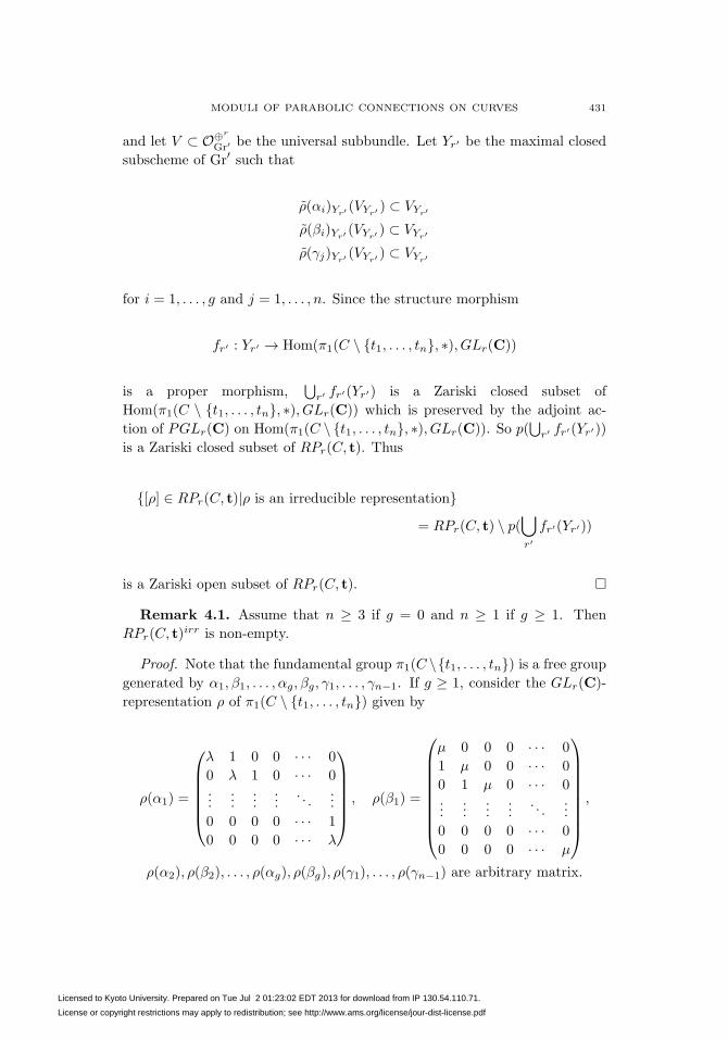
Remark 4.1. Assume that n ≥ 3 if g = 0 and n ≥ 1 if g ≥ 1. Then
RPr(C, t)irr is non-empty.
Proof. Note that the fundamental group π1(C \{t1, . . . , tn}) is a free group
generated by α1, β1, . . . , αg, βg, γ1, . . . , γn−1. If g ≥ 1, consider the GLr(C)-
representation ρ of π1(C \ {t1, . . . , tn}) given by
ρ(α1) =
⎛⎜⎜⎜⎜⎜⎝
λ 1 0 0 · · · 0
0 λ 1 0 · · · 0...
......
.... . .
...
0 0 0 0 · · · 1
0 0 0 0 · · · λ
⎞⎟⎟⎟⎟⎟⎠ , ρ(β1) =
⎛⎜⎜⎜⎜⎜⎜⎜⎜⎝
μ 0 0 0 · · · 0
1 μ 0 0 · · · 0
0 1 μ 0 · · · 0...
......
.... . .
...
0 0 0 0 · · · 0
0 0 0 0 · · · μ
⎞⎟⎟⎟⎟⎟⎟⎟⎟⎠
,
ρ(α2), ρ(β2), . . . , ρ(αg), ρ(βg), ρ(γ1), . . . , ρ(γn−1) are arbitrary matrix.
Licensed to Kyoto University. Prepared on Tue Jul 2 01:23:02 EDT 2013 for download from IP 130.54.110.71.
License or copyright restrictions may apply to redistribution; see http://www.ams.org/license/jour-dist-license.pdf
432 MICHI-AKI INABA
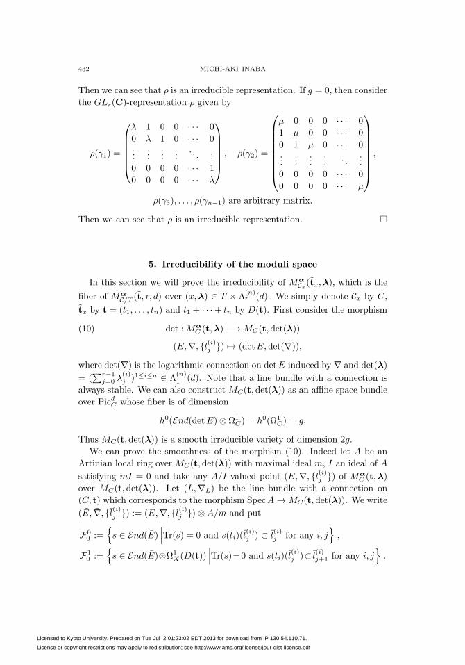
Then we can see that ρ is an irreducible representation. If g = 0, then consider
the GLr(C)-representation ρ given by
ρ(γ1) =
⎛⎜⎜⎜⎜⎜⎝
λ 1 0 0 · · · 0
0 λ 1 0 · · · 0...
......
.... . .
...
0 0 0 0 · · · 1
0 0 0 0 · · · λ
⎞⎟⎟⎟⎟⎟⎠ , ρ(γ2) =
⎛⎜⎜⎜⎜⎜⎜⎜⎜⎝
μ 0 0 0 · · · 0
1 μ 0 0 · · · 0
0 1 μ 0 · · · 0...
......
.... . .
...
0 0 0 0 · · · 0
0 0 0 0 · · · μ
⎞⎟⎟⎟⎟⎟⎟⎟⎟⎠
,
ρ(γ3), . . . , ρ(γn−1) are arbitrary matrix.
Then we can see that ρ is an irreducible representation. �
5. Irreducibility of the moduli space
In this section we will prove the irreducibility of MαCx(tx,λ), which is the
fiber of MαC/T (t, r, d) over (x,λ) ∈ T × Λ
(n)r (d). We simply denote Cx by C,
tx by t = (t1, . . . , tn) and t1 + · · ·+ tn by D(t). First consider the morphism
det : MαC (t,λ) −→ MC(t, det(λ))(10)
(E,∇, {l(i)j }) �→ (detE, det(∇)),
where det(∇) is the logarithmic connection on detE induced by ∇ and det(λ)
= (∑r−1
j=0 λ(i)j )1≤i≤n ∈ Λ
(n)1 (d). Note that a line bundle with a connection is
always stable. We can also construct MC(t, det(λ)) as an affine space bundle
over PicdC whose fiber is of dimension
h0(End(detE)⊗ Ω1C) = h0(Ω1
C) = g.
Thus MC(t, det(λ)) is a smooth irreducible variety of dimension 2g.
We can prove the smoothness of the morphism (10). Indeed let A be an
Artinian local ring over MC(t, det(λ)) with maximal ideal m, I an ideal of A
satisfying mI = 0 and take any A/I-valued point (E,∇, {l(i)j }) of MαC (t,λ)
over MC(t, det(λ)). Let (L,∇L) be the line bundle with a connection on
(C, t) which corresponds to the morphism SpecA → MC(t, det(λ)). We write
(E, ∇, {l(i)j }) := (E,∇, {l(i)j })⊗A/m and put
F00 :=
{s ∈ End(E)
∣∣∣Tr(s) = 0 and s(ti)(l(i)j ) ⊂ l
(i)j for any i, j
},
F10 :=
{s ∈ End(E)⊗Ω1
X(D(t))∣∣∣Tr(s)=0 and s(ti)(l
(i)j )⊂ l
(i)j+1 for any i, j
}.
Licensed to Kyoto University. Prepared on Tue Jul 2 01:23:02 EDT 2013 for download from IP 130.54.110.71.
License or copyright restrictions may apply to redistribution; see http://www.ams.org/license/jour-dist-license.pdf
MODULI OF PARABOLIC CONNECTIONS ON CURVES 433
We define a complex F•0 by
∇F•0: F0
0 � s �→ ∇ ◦ s− s ◦ ∇ ∈ F10 .
Then the obstruction class for the lifting of (E,∇, {l(i)j }) to an A-valued point
(E, ∇, {l(i)j }) of MαC (t,λ) with (det(E), det(∇)) ∼= (L,∇L) lies in H2(F•
0 )⊗I.
Using the same method as in the proof of Theorem 2.1, we can see that
H2(F•0 )
∼=(ker(H0(F0
0 ) → H0(F10 )))∨
and we can see by the stability of (E, ∇, {l(i)j }) that ker(H0(F00 ) → H0(F1
0 )) =
0. Hence the morphism det in (10) is smooth.
From the above argument, it is sufficient to prove the irreducibility of the
fibers of the morphism (10) det : MαC (t,λ) → MC(t, det(λ)) in order to
obtain the irreducibility of MαC (t,λ). So we fix a line bundle L on C and a
connection
∇L : L −→ L⊗ Ω1C(t1 + · · ·+ tn).
We set
MαC (t,λ, L) :=
{(E,∇, {l(i)j }) ∈ Mα
C (t,λ)∣∣∣ (detE, det(∇)) ∼= (L,∇L)
}.
Then MαC (t,λ, L) is smooth of equidimension (r − 1)(2(r + 1)(g − 1) + rn).
Proposition 5.1. Assume that g ≥ 2 and n ≥ 1. Then MαC (t,λ, L) is an
irreducible variety of dimension (r − 1)(2(r + 1)(g − 1) + rn).
Proof. By taking the elementary transform, we can obtain an isomorphism
σ : MC(t,λ, L)∼−→ MC(t,λ
′, L′),
with r and detL′ coprime. Consider the open subscheme
N :={(E,∇, {l(i)j }) ∈ Mα
C (t,λ, L)∣∣∣σ(E) is a stable vector bundle
}of Mα
C (t,λ, L).
Step 1. We will see that N is irreducible.
Let MC(r, L′) be the moduli space of stable vector bundles of rank r with
the determinant L′. As is well known, MC(r, L′) is a smooth irreducible
variety and there is a universal bundle E on C×MC(r, L′). Note that there is
a line bundle L on MC(r, L′) such that det(E) ∼= L⊗L. We can parameterize
the parabolic structures on Es (s ∈ MC(r, L′)) by a product of flag schemes
U :=
n∏i=1
Flag(E|ti×MC(r,L′)),
which is obviously smooth and irreducible. Let {l(i)j } be the universal family
over U , where
EU |ti×U = l(i)0 ⊃ l
(i)1 ⊃ · · · ⊃ l
(i)r−1 ⊃ l(i)r = 0
Licensed to Kyoto University. Prepared on Tue Jul 2 01:23:02 EDT 2013 for download from IP 130.54.110.71.
License or copyright restrictions may apply to redistribution; see http://www.ams.org/license/jour-dist-license.pdf
434 MICHI-AKI INABA
is the filtration by subbundles for i = 1, . . . , n such that dim(l(i)j )s/(l
(i)j+1)s = 1
for any i, j and s ∈ U . Consider the functor ConnU : (Sch/U) → (Sets)
defined by
ConnU (S)=
⎧⎪⎪⎪⎨⎪⎪⎪⎩∇ : ES → ES ⊗ Ω1
C(D(t))
∣∣∣∣∣∣∣∣∣∇ is a relative connection
satisfying (resti×S(∇)−λ(i)j )(l
(i)j )S
⊂ (l(i)j+1)S for any i, j and det(∇)
= (∇L)S ⊗ LS
⎫⎪⎪⎪⎬⎪⎪⎪⎭ .
We can define a morphism of functors
ConnU −→ QuotΛ1D(t)
⊗E/C×U/U
∇ �→[Λ1D(t) ⊗ EU � (a, v)⊗ e �→ ae+∇v(e) ∈ EU
],
which is representable by an immersion. So there is a locally closed subscheme
Y of QuotΛ1D(t)
⊗E/C×U/U which represents the functor ConnU . We will show
that Y is smooth over U . So let ∇ : EY → EY ⊗ Ω1C(D(t)) be the universal
connection and put
F00 :=
{s ∈ End(E)
∣∣∣Tr(s) = 0 and s|ti×Y ((l(i)j )Y ) ⊂ (l
(i)j )Y for any i, j
},
F10 :=
{s ∈ End(E)⊗ Ω1
C(D(t))∣∣∣Tr(s) = 0 and resti×Y (s)((l
(i)j )Y )
⊂ (l(i)j+1)Y for any i, j
},
∇F•0: F0
0 � s �→ ∇ ◦ s− s ◦ ∇ ∈ F10 .
Let A be an Artinian local ring over U with maximal ideal m and I an ideal
of A satisfying mI = 0. Take any A/I-valued point x of Y over U . We put
x := x⊗ A/m. Then the obstruction class for the lifting of x to an A-valued
point of Y lies in H1(F10 ⊗ k(x)) ⊗ I. We can see that H1(F1
0 ⊗ k(x)) ∼=H0(F0
0 ⊗ k(x))∨ = 0 because E ⊗ k(x) is a stable bundle. Thus Y is smooth
over U . We can see that the fiber Ys of any point s ∈ U is isomorphic to the
affine space isomorphic to H0(F10 ⊗ k(s)). So Y is irreducible. Consider the
open subscheme
Y ′ :={x ∈ Y
∣∣∣σ−1(Ex, ∇ ⊗ k(x), {(l(i)j )x}) is α-stable}
of Y . Then we obtain a morphism Y ′ → MαC (t,λ, L) whose image is just N .
Thus N is irreducible.
Step 2.
dim(MαC (t,λ, L) \N) < dimMα
C (t,λ, L) = (r − 1)(2(r + 1)(g − 1) + rn).
Licensed to Kyoto University. Prepared on Tue Jul 2 01:23:02 EDT 2013 for download from IP 130.54.110.71.
License or copyright restrictions may apply to redistribution; see http://www.ams.org/license/jour-dist-license.pdf
MODULI OF PARABOLIC CONNECTIONS ON CURVES 435
For the proof of Step 2, it is sufficient to show that there is an algebraic
scheme B with dim B < (r − 1)(2(r + 1)(g − 1) + rn) and a surjection B →σ(Mα
C (t,λ, L) \N). Take any member (E,∇E, {l(i)j }) ∈ σ(MαC (t,λ, L) \N).
Let
0 = E0 ⊂ E1 ⊂ E2 ⊂ · · · ⊂ Es = E
be the Harder-Narasimhan filtration of E. Note that s > 1 because r and
degE = degL′ are coprime. Put Ek := Ek/Ek−1 for k = 1, . . . , s. For each
Ek, there is a Jordan-Holder filtration
0 = E(0)k ⊂ E
(1)k ⊂ E
(2)k ⊂ · · · ⊂ E
(mk)k = Ek.
We put E(i)k := E
(i)k /E
(i−1)k for i = 1, . . . ,mk. Put r
(j)k = rank E
(j)k and d
(j)k =
deg E(j)k . We can parameterize each E
(j)k by the moduli space M(r
(j)k , d
(j)k )
of stable bundles of rank r(j)k and degree d
(j)k whose dimension is
dimExt1(E(j)k , E
(j)k ). Replacing M(r
(j)k , d
(j)k ) by an etale covering, we may
assume that there is a universal bundle E(j)k on C ×M(r
(j)k , d
(j)k ). If we put
X :=
⎧⎨⎩(x
(j)k ) ∈
∏1≤k≤s,1≤j≤mk
M(r(j)k , d
(j)k )
∣∣∣∣∣∣⊗j,k
det(E(j)k
)x(j)k
∼= L
⎫⎬⎭ ,
then X is smooth of dimension −g +∑s
k=1
∑mk
j=1 dimExt1(E(j)k , E
(j)k ). Re-
placing X by its stratification, we may assume that the relative Ext-sheaf
Ext1C×X/X(E(2)k , E(1)
k ) becomes locally free. We put W(2)k := X and E(2)
k :=
E(1)k ⊕ E(2)
k if the extension
0 −→ E(1)k −→ E
(2)k −→ E
(2)k −→ 0
splits. Otherwise we put
W(2)k := P∗
(Ext1C×X/X(E(2)
k , E(1)k ))
and take a universal extension
0 −→ (E(1)k )
W(2)k
⊗ L(2)k −→ E(2)
k −→ (E(2)k )
W(2)k
−→ 0
for some line bundle L(2)k on W
(2)k . We define W
(j)k and E(j)
k inductively on
j as follows: Replacing W(j−1)k by its stratification, we may assume that
the relative Ext-sheaf Ext1C×W
(j−1)k /W
(j−1)k
((E(j)k )
W(j−1)k
, E(j−1)k ) is locally free.
Then put W(j)k := W
(j−1)k and E(j)
k := E(j−1)k ⊕ (E(j)
k )W
(j)k
if the extension
0 −→ E(j−1)k −→ E
(j)k −→ E
(j)k −→ 0
Licensed to Kyoto University. Prepared on Tue Jul 2 01:23:02 EDT 2013 for download from IP 130.54.110.71.
License or copyright restrictions may apply to redistribution; see http://www.ams.org/license/jour-dist-license.pdf
436 MICHI-AKI INABA
splits; otherwise, we put
W(j)k := P∗
(Ext1
C×W(j−1)k /W
(j−1)k
((E(j)k )
W(j−1)k
, E(j−1)k )
)and take a universal extension
0 −→ (E(j−1)k )
W(j)k
⊗ L(j)k −→ E(j)
k −→ (E(j)k )
W(j)k
−→ 0
for some line bundle L(j)k on W
(j)k . We can see by the construction that
the relative dimension of W(mk)k over X at the point corresponding to the
extensions
0 −→ E(j−1)k −→ E
(j)k −→ E
(j)k −→ 0 (j = 2, . . . ,mk, E
(1)k = E
(1)k )
is at most 1−mk +∑
1≤i<j≤mkdimExt1(E
(j)k , E
(i)k ). We put
W := W(m1)1 ×X · · · ×X W (ms)
s
and Ek := (E(mk)k )W for k = 1, . . . , s. Replacing W by its stratification, we
assume that the relative Ext-sheaf Ext1C×W/W (E2, E1) is locally free. Then we
put W2 := W and E2 := E1 ⊕ E2 if the extension
0 −→ E1 −→ E2 −→ E2 −→ 0
splits and otherwise we put
W2 := P∗(Ext1C×W/W (E2, E1)
)and take a universal extension
0 −→ (E1)W2⊗ L2 −→ E2 −→ (E2)W2
−→ 0
for some line bundle L2. We define Wk and Ek inductively as follows: Re-
placing Wk−1 by its stratification, we assume that the relative Ext-sheaf
Ext1C×Wk−1/Wk−1((Ek)Wk−1
, Ek−1) is locally free. Then we put Wk := Wk−1
and Ek := Ek ⊕ Ek−1 if the extension
0 −→ Ek−1 −→ Ek −→ Ek −→ 0
splits and otherwise we put
Wk := P∗
(Ext1C×Wk−1/Wk−1
((Ek)Wk−1, Ek−1)
)and take a universal extension
0 −→ (Ek−1)Wk⊗ Lk −→ Ek −→ (Ek)Wk
−→ 0
for some line bundle Lk on Wk. We put rk := rank Ek for k = 1, . . . , s.
Claim. dimExt1(Ek, Ek′) < rkrk′(2g − 2) for k′ < k.
Take a general point t ∈ C. We prove this claim in the following three
cases.
Licensed to Kyoto University. Prepared on Tue Jul 2 01:23:02 EDT 2013 for download from IP 130.54.110.71.
License or copyright restrictions may apply to redistribution; see http://www.ams.org/license/jour-dist-license.pdf
MODULI OF PARABOLIC CONNECTIONS ON CURVES 437
Case 1. deg(E∨k′ ⊗ Ek(t)) > 0.
By the Riemann-Roch theorem, we have
dimHom(Ek(t), Ek′)− dimH0((Ek′)∨ ⊗ Ek(t)⊗ ωC)
= rk′rk(1− g) + deg((Ek(t))∨ ⊗ Ek′).
Here we have Hom(Ek(t), Ek′) = 0 because Ek(t) and Ek′ are semistable and
deg((Ek(t))∨ ⊗ Ek′) < 0. So we have
dimExt1(Ek, Ek′) = dimH0(E∨k′ ⊗ Ek ⊗ ωC)
≤ dimH0(E∨k′ ⊗ Ek(t)⊗ ωC)
= rkrk′(g − 1)− deg((Ek(t))∨ ⊗ Ek′)
< rkrk′(g − 1) + rkrk′
≤ rkrk′(2g − 2).
Case 2. deg(E∨k′ ⊗ Ek(t)) < 0.
Note that there is an exact sequence
0 −→ H0(E∨k′ ⊗ Ek ⊗ ωC(−p1 − · · · − p2g−3))
−→ H0(E∨k′ ⊗ Ek ⊗ ωC(−p1 − · · · − p2g−4))
−→ H0(E∨k′ ⊗ Ek ⊗ ωC(−p1 − · · · − p2g−4)|p2g−3
) ∼= Crkrk′ .
Since deg(E∨k′⊗Ek⊗ωC(−p1−· · ·−p2g−3)) < 0 and Ek and Ek′ are semistable,
we have
H0(E∨k′ ⊗ Ek ⊗ ωC(−p1 − · · · − p2g−3)) = 0.
So we have dimH0(E∨k′ ⊗ Ek ⊗ ωC(−p1 − · · · − p2g−4)) ≤ rkrk′ . Inductively
we can see that
dimH0(E∨k′ ⊗ Ek ⊗ ωC(−p1 − · · · − p2g−2−m)) ≤ rkrk′(m− 1)
for 2 ≤ m ≤ 2g − 2, because there are exact sequences
0 −→ H0(E∨k′ ⊗ Ek ⊗ ωC(−p1 − · · · − p2g−2−m+1))
−→ H0(E∨k′ ⊗ Ek ⊗ ωC(−p1 − · · · − p2g−2−m))
−→ H0(E∨k′ ⊗ Ek ⊗ ωC(−p1 − · · · − p2g−2−m)|p2g−2−m+1
) ∼= Crkrk′
for 2 ≤ m ≤ 2g − 2. Thus we have
dimExt1(Ek, Ek′) = dimH0(E∨k′ ⊗ Ek ⊗ ωC) ≤ rkrk′(2g − 3).
Case 3. deg(E∨k′ ⊗ Ek(t)) = 0.
Licensed to Kyoto University. Prepared on Tue Jul 2 01:23:02 EDT 2013 for download from IP 130.54.110.71.
License or copyright restrictions may apply to redistribution; see http://www.ams.org/license/jour-dist-license.pdf

438 MICHI-AKI INABA
Put F := E∨k′ ⊗ Ek⊗ωC(−p1−· · ·−p2g−3). Then F is semistable of degree
0. Let 0 = F0 ⊂ F1 ⊂ · · · ⊂ Fl = F be a Jordan-Holder filtration of F . If we
put t ∈ C sufficiently general, we may assume that OC(t− p2g−3) �∼= Fi/Fi−1
for any i. Then we have
Hom(OC(t− p2g−3), E∨k′ ⊗ Ek ⊗ ωC(−p1 − · · · − p2g−3)) = 0.
Since there is an exact sequence
0 = H0(E∨k′ ⊗ Ek ⊗ ωC(−p1 − · · · − p2g−4 − t))
−→ H0(E∨k′ ⊗ Ek ⊗ ωC(−p1 − · · · − p2g−4))
−→ H0(E∨k′ ⊗ Ek ⊗ ωC(−p1 − · · · − p2g−4)|t) ∼= Crkrk′ ,
we have dimH0(E∨k′ ⊗ Ek ⊗ ωC(−p1 − · · · − p2g−4)) ≤ rkrk′ . Inductively we
can see that
dimH0(E∨k′ ⊗ Ek ⊗ ωC(−p1 − · · · − p2g−2−m)) ≤ rkrk′(m− 1)
for 2 ≤ m ≤ 2g−2. So we have dimExt1(Ek, Ek′) = dimH0(E∨k′⊗Ek⊗ωC) ≤
rkrk′(2g − 3).
Thus the claim has been proved.
We can see that the relative dimension of Wk over Wk−1 at the point
corresponding to the extension
0 −→ Ek−1 −→ Ek −→ Ek −→ 0
is at most
dimExt1(Ek, Ek−1)− 1 ≤ −1 +∑
k′≤k−1
dimExt1(Ek, Ek′)
< −1 +∑
1≤k′<k
(rk′rk(2g − 2))
if 0 → Ek−1 → Ek → Ek → 0 does not split. If the extension 0 → Ek−1 →Ek → Ek → 0 splits, the relative dimension of Wk over Wk−1 is at most
−1 +∑
1≤k′<k rk′rk(2g − 2). Then we can see that the dimension of Ws at
the point corresponding to the extensions
0 = E0 ⊂ E1 ⊂ · · · ⊂ Es = E, Ek = Ek/Ek−1,
0 = E(0)k ⊂ E
(1)k ⊂ · · · ⊂ E
(mk)k = Ek, E
(j)k = E
(j)k /E
(j−1)k ,
Licensed to Kyoto University. Prepared on Tue Jul 2 01:23:02 EDT 2013 for download from IP 130.54.110.71.
License or copyright restrictions may apply to redistribution; see http://www.ams.org/license/jour-dist-license.pdf
MODULI OF PARABOLIC CONNECTIONS ON CURVES 439
is at most
− g +s∑
k=1
mk∑j=1
dimExt1(E(j)k , E
(j)k )
+s∑
k=1
⎛⎝1−mk +
∑1≤i<j≤mk
dimExt1(E(j)k , E
(i)k )
⎞⎠
+
s∑k=2
⎛⎝−1 +
∑1≤k′<k
dimExt1(Ek, Ek′)
⎞⎠
<− g +
s∑k=1
mk∑j=1
dimExt1(E(j)k , E
(j)k )
+
s∑k=1
⎛⎝1−mk +
∑1≤i<j≤mk
dimExt1(E(j)k , E
(i)k )
⎞⎠
+ 1− s+∑
1≤k′<k≤s
rk′rk(2g − 2)
≤s∑
k=1
mk∑i=1
((r(i)k )2(g − 1) + 1) +
s∑k=1
⎛⎝1−mk +
∑1≤i<j≤mk
(r(i)k r
(j)k (g − 1) + 1)
⎞⎠
− g + 1− s+∑
1≤k′<k≤s
∑1≤i≤mk,1≤j≤mk′
r(i)k r
(j)k′ (2g − 2)
≤s∑
k=1
mk∑i=1
(r(i)k )2(g − 1) +
s∑k=1
∑1≤i<j≤mk
2r(i)k r
(j)k (g − 1)
− g + 1 +∑k<k′
∑1≤i≤mk,1≤j≤mk′
2r(i)k′ r
(j)k (g − 1)
=(r2 − 1)(g − 1)
because we have s > 1.
Consider the product of flag schemes
Z :=n∏
i=1
Flag(Es|ti×Ws)
over Ws and put E := (Es)Z . Then there is a universal parabolic structure
E|ti×Z = l(i)0 ⊃ l
(i)1 ⊃ · · · ⊃ l
(i)r−1 ⊃ l(i)r = 0
Licensed to Kyoto University. Prepared on Tue Jul 2 01:23:02 EDT 2013 for download from IP 130.54.110.71.
License or copyright restrictions may apply to redistribution; see http://www.ams.org/license/jour-dist-license.pdf
440 MICHI-AKI INABA
for each i = 1, . . . , n. The dimension of Z at the point corresponding to the
extensions
0 = E0 ⊂ E1 ⊂ · · · ⊂ Es = E, Ek = Ek/Ek−1,
0 = E(0)k ⊂ E
(1)k ⊂ · · · ⊂ E
(mk)k = Ek, E
(j)k = E
(j)k /E
(j−1)k ,
and the parabolic structure
E|ti = l(i)0 ⊃ l
(i)1 ⊃ · · · ⊃ l
(i)r−1 ⊃ l(i)r = 0 (i = 1, . . . , n)
is less than (r2 − 1)(g − 1) + r(r − 1)n/2 = (r − 1)((r + 1)(g − 1) + rn/2).
Consider the functor ConnZ : (Sch/Z) → (Sets) defined by
ConnZ(S) =
⎧⎪⎪⎪⎪⎪⎪⎪⎪⎪⎨⎪⎪⎪⎪⎪⎪⎪⎪⎪⎩∇ : ES → ES ⊗ Ω1
C(D(t))
∣∣∣∣∣∣∣∣∣∣∣∣∣∣∣
∇ is a connection such that
(resti×S(∇)− λ(i)j )((l
(i)j )S)
⊂ (l(i)j+1)S for any i, j
and det(∇) = ∇L ⊗ Lvia an identification E =
L⊗ L for some line bundle
L on S
⎫⎪⎪⎪⎪⎪⎪⎪⎪⎪⎬⎪⎪⎪⎪⎪⎪⎪⎪⎪⎭
.
We can see that ConnZ can be represented by a scheme B of finite type over
Z. Let
∇ : EB −→ EB ⊗ Ω1C(D(t))
be the universal connection. If we put
F00 :=
{u ∈ End(E)
∣∣∣Tr(u) = 0 and u|ti×Y ((l(i)j )Y ) ⊂ (l
(i)j )Y for any i, j
},
F10 :=
{u ∈ End(E)⊗ Ω1
C(D(t)) |Tr(u) = 0 and
resti×Y (u)((l(i)j )Y ) ⊂ (l
(i)j+1)Y for any i, j
},
∇F•0: F0
0 :� u �→ ∇F•0◦ u− u ◦ ∇F• ∈ F1
0 ,
then the fiber Bx of B over x ∈ Z is isomorphic to the affine space
H0(F10 ⊗ k(x)). Put
B′ :={x ∈ B
∣∣∣σ−1(Ex, ∇ ⊗ k(x),
{l(i)j ⊗ k(x)
})is α-stable
}.
Then there is a canonical morphism
ψ : B′ −→ MαC (t,λ, L) \N
and the homomorphism
H0(∇F•0⊗ k(x)) : H0(F0
0 ⊗ k(x)) −→ H0(F10 ⊗ k(x))
Licensed to Kyoto University. Prepared on Tue Jul 2 01:23:02 EDT 2013 for download from IP 130.54.110.71.
License or copyright restrictions may apply to redistribution; see http://www.ams.org/license/jour-dist-license.pdf
MODULI OF PARABOLIC CONNECTIONS ON CURVES 441
is injective for x ∈ B′, because End(E ⊗ k(x), ∇ ⊗ k(x), {l(i)j ⊗ k(x)}) ∼= k(x).
If we put
U :={u : E⊗k(x)
∼−→E⊗k(x)∣∣∣u(l(i)j ⊗k(x))⊂ l
(i)j ⊗k(x) and
∧ru=id
},
for x ∈ Z, then we have a morphism
ι : U → B′x; u �→ u ◦ (∇ ⊗ k(x)) ◦ u−1.
We can see that the tangent map of ι at id is just the homomorphism
H0(∇F•0⊗ k(x)) which is injective. We may assume that the morphism
ψ : B′ → ψ(B′) is flat by replacing B′ by a disjoint union of subschemes.
So we have for any x ∈ B′,
dimψ(x) ψ(B′) = dimx(B′)− dimx ψ
−1(ψ(x))
≤ dim(Z) + dimx B′x − dimx ι(U)
≤ dim(Z) + dimH0(F10 ⊗ k(x))− dimH0(F0
0 ⊗ k(x))
< (r − 1)(2(r + 1)(g − 1) + rn),
because
dim coker(H0(F00 ⊗ k(x)) → H0(F1
0 ⊗ k(x))) = (r− 1)((r+1)(g− 1)+ rn/2).
Note that MαC (t,λ, L) \ N can be covered by a finite union of such ψ(B′)s;
hence, we have
dim(MαC (t,λ, L) \N) < (r − 1)(2(r + 1)(g − 1) + rn).
So Step 2 is proved. By Step 1, Step 2 and the fact that the moduli space
MαC (t,λ, L) is smooth of equidimension (r − 1)(2(r + 1)(g − 1) + rn), the
moduli space MαC (t,λ, L) is irreducible. �
Proposition 5.2. Assume that g = 1 and n ≥ 2. Then MαC (t,λ, L) is an
irreducible variety of dimension r(r − 1)n.
Proof. Composing certain elementary transforms, we obtain an isomor-
phism
σ : MC(t,λ, L)∼−→ MC(t,λ
′, L′),
where r and degL′ are coprime. Put
N :={(E,∇, {l(i)j }) ∈ Mα
C (t,λ, L)∣∣∣σ(E) is a stable bundle
}.
As in the proof of the previous proposition, we can show that N is irre-
ducible. So it suffices to show that dim(MαC (t,λ, L) \ N) < r(r − 1)n be-
cause MαC (t,λ, L) is smooth of equidimension r(r − 1)n. Take any member
(E,∇, {l(i)j }) ∈ σ(MαC (t,λ, L) \ N). Let Fs ⊂ Fs−1 ⊂ · · · ⊂ F1 = E be the
Licensed to Kyoto University. Prepared on Tue Jul 2 01:23:02 EDT 2013 for download from IP 130.54.110.71.
License or copyright restrictions may apply to redistribution; see http://www.ams.org/license/jour-dist-license.pdf
442 MICHI-AKI INABA
Harder-Narasimhan filtration of E. Note that s > 1. We can inductively see
that the extension
0 −→ Fp/Fp+1 −→ E/Fp+1 −→ E/Fp −→ 0
must split for p = 2, . . . , s, where we put Fs+1 = 0. Then we have a decompo-
sition E ∼= E1 ⊕ · · · ⊕ Es, where each Ep is semistable and μ(E1) < μ(E2) <
· · · < μ(Es). We can write Ep =⊕rp
j=1 Fp,j , where each Fp,j is a successive
extension of a stable bundle F(j)p and F
(j)p �∼= F
(k)p for j �= k. We can see that
Fp,j∼= G1 ⊕ · · · ⊕ Gm, where each Gi is a successive non-split extension of
F(j)p . We put r
(j)p := rankF
(j)p and d
(j)p := degF
(j)p . Let MC(r
(j)p , d
(j)p ) be the
moduli space of stable bundles on C of rank r(j)p and degree d
(j)p . Replacing
MC(r(j)p , d
(j)p ) by an etale covering, we may assume that there is a universal
bundle F (j)p on C × MC(r
(j)p , d
(j)p ). We can construct non-split extensions
G1, . . . ,Gm of F (j)p such that Fp,j
∼= (G1 ⊕ · · · ⊕ Gm)⊗ k(x0) for the point x0
of MC(r(j)p , d
(j)p ) corresponding to F
(j)p . We put Fp,j := G1 ⊕ · · · ⊕ Gm and
W :=
⎧⎨⎩(x(j)
p ) ∈∏
1≤p≤s,1≤j≤rp
MC(r(j)p , d(j)p )
∣∣∣∣∣∣⊗p,j
det(Fp,j ⊗ k(x(j)
p ))∼= L
⎫⎬⎭ .
Then dimW = −1 +∑s
p=1 rp. We put E :=⊕
j,p Fp,j . Then parabolic
structure can be parameterized by the product of flag schemes
U :=n∏
i=1
Flag(E|ti×W )
over W . The relative dimension of U over W is r(r− 1)n/2. Let {l(i)j } be the
universal parabolic structure on EU . Note that
End(E⊗k(x))=s⊕
p=1
rp⊕j=1
End(Fp,j⊗k(x))⊕⊕p<q
⊕j,k
Hom(Fp,j⊗k(x),Fq,k⊗k(x))
for a point x ∈ W and the group
Gx :=
⎧⎨⎩∑
p,j
cpj idFp,j⊗k(x) +∑p<q
∑j,k
a(p,q)j,k
∈ End(E ⊗ k(x))
∣∣∣∣∣ cpj ∈ C∗,
a(p,q)j,k ∈ Hom(Fp,j ⊗ k(x),Fq,k ⊗ k(x))
⎫⎬⎭
acts on the fiber Ux of U over x. Note that we can take a section a ∈Hom(Fp,j ⊗ k(x),Fq,k ⊗ k(x)) with a(t1) �= 0 or a(t2) �= 0 if p < q. So we
Licensed to Kyoto University. Prepared on Tue Jul 2 01:23:02 EDT 2013 for download from IP 130.54.110.71.
License or copyright restrictions may apply to redistribution; see http://www.ams.org/license/jour-dist-license.pdf
MODULI OF PARABOLIC CONNECTIONS ON CURVES 443
may assume that α(t2) �= 0 for some α ∈ Hom(Fp0,1 ⊗ k(x),Fp0+1,1 ⊗ k(x)).
Modulo the action of the group⎧⎨⎩∑
p,j
cpj idFp,j⊗ k(x)
∣∣∣∣∣∣ cpj ∈ C×
⎫⎬⎭ ,
l(1)r−1 ⊗ k(y) (y ∈ Ux) can be parameterized by an algebraic scheme whose
dimension is at most r−∑s
p=1 rp. Moreover, modulo the action of the group⎧⎨⎩idE⊗k(x) +
∑p<q
∑j,k
a(p,q)j,k
∣∣∣∣∣∣ a(p,q)j,k ∈ Hom(Fp,j ⊗ k(x),Fq,k ⊗ k(x))
⎫⎬⎭ ,
l(2)r−1 ⊗ k(y) (y ∈ Ux) can be parameterized by an algebraic scheme whose
dimension is at most r − 2. Then, modulo the action of Gx, l(1)r−1 ⊗ k(y) and
l(2)r−1 ⊗ k(y) (y ∈ Ux) can be parameterized by an algebraic scheme whose
dimension is at most 2r −∑s
p=1 rp − 2. So we can take a finite number of
subschemes Y1, . . . , Yl of U such that dimYi ≤ −1 +∑s
p=1 rp + r(r− 1)n/2−∑sp=1 rp = r(r− 1)n/2− 1 and
⋃li=1 Gx(Yi)x = Ux for any point x ∈ W . We
put Y :=∐l
i=1 Yi. Replacing Y by its stratification, we may assume that the
dimension of
F 0y :=
{s ∈ End(Ey)
∣∣∣Tr(s) = 0 and s(ti)(l(i)j )y ⊂ (l
(i)j )y for each i, j
}is constant for y ∈ Y . There exists a scheme Z over Y such that for any
Y -scheme S, we have
Z(S) =
⎧⎪⎪⎪⎨⎪⎪⎪⎩∇ : ES → ES⊗Ω1
C(t1 + · · ·+ tn)
∣∣∣∣∣∣∣∣∣∇ is a relative connection such
that (resti×S(∇)− λ(i)j )((l
(i)j )S)
⊂ (l(i)j+1)S for any i, j and
det(∇) = (∇L)⊗ L
⎫⎪⎪⎪⎬⎪⎪⎪⎭.
We can see that each fiber of Z → Y over y ∈ Y is an affine space isomorphic
to
F 1y =
{s ∈ Hom(Ey, Ey ⊗ Ω1
C(t1 + · · ·+ tn)) |Tr(s) = 0 and
resti(s)(l(i)j )y ⊂ (l
(i)j+1)y for any i, j
}.
Let ∇ : EZ → EZ ⊗ Ω1C(t1 + · · ·+ tn) be the universal relative connection. If
we put
Zs :={y ∈ Z
∣∣∣σ−1((E , ∇, {l(i)j })⊗ k(y)
)is α-stable
},
Licensed to Kyoto University. Prepared on Tue Jul 2 01:23:02 EDT 2013 for download from IP 130.54.110.71.
License or copyright restrictions may apply to redistribution; see http://www.ams.org/license/jour-dist-license.pdf
444 MICHI-AKI INABA
then there is a natural morphism f : Zs → MαC (t,λ, L). For each z ∈ Z over
y ∈ Y , consider the homomorphism
∇1z : F 0
y ⊗ k(z) −→ F 1y ⊗ k(z); ∇1
z(s) := ∇z ◦ s− s ◦ ∇z.
Then the group Staby of automorphisms g of the parabolic bundles (Ey,{(l(i)j )y}) which induce the identity on det(Ey) acts on the fiber Zy and the
tangent map of the morphism Staby � g �→ gz ∈ Zs at id is just the homo-
morphism ∇1z which is injective. Replacing Zs by a finite disjoint union of
subschemes, we may assume that Zs f→ f(Zs) is flat. Then we have
dimf(z) f(Zs) = dimz Zs − dimz f
−1(f(z))
≤ dimz Zs − dimid Staby
= dimz Zs − dimF 0
y
≤ dimy Y + dimz Zsy − dimF 0
y
≤ dimy Y + dimF 1y − dimF 0
y
≤ dimY + r(r − 1)n/2 ≤ r(r − 1)n− 1.
Here z ∈ Zs and Zs � z �→ y ∈ Y . Since MαC (t,λ, L) \N is a finite union of
such f(Zs)s, we have dim(MαC (t,λ, L) \N) < r(r − 1)n. �
Proposition 5.3. Assume that rn − 2(r + 1) > 0 and r ≥ 2. Then
MαP1(t,λ, L) is an irreducible variety of dimension (r − 1)(rn− 2r − 2).
Proof. First we will show that the Zariski open set
N :={(E,∇, {l(i)j }) ∈ Mα
P1(t,λ, L)∣∣∣ dimEnd(E, {l(i)j }) = 1
}is irreducible. There exists an integer n0 such that h1(E(n0)) = 0 for any
(E,∇, {l(i)j }) ∈ MαP1(t,λ, L). Then we can easily construct a smooth irre-
ducible variety X and a flat family of parabolic bundles (E, {l(i)j }) on P1×X
over X whose geometric fibers is just the set of all the simple parabolic bun-
dles (E, {l(i)j }) satisfying h1(E(n0)) = 0 and detE = L. We can take an
isomorphism det E ∼= L ⊗ L for some line bundle L on X. The functor
ConnX : (Sch/X) −→ (Sets) defined by
ConnX(U) =
⎧⎪⎪⎪⎪⎪⎨⎪⎪⎪⎪⎪⎩∇ : EU → EU ⊗ Ω1
P1(D(t))
∣∣∣∣∣∣∣∣∣∣∣
∇ is a relative connection
satisfying (resti(∇)
−λ(i)j )((l
(i)j )U ) ⊂ (l
(i)j+1)U
for any i, j and
det(∇) = (∇L)U ⊗ L
⎫⎪⎪⎪⎪⎪⎬⎪⎪⎪⎪⎪⎭
is represented by a scheme Y of finite type over X. We can see by the same
proof as Proposition 5.1 that Y is smooth over X whose fiber is an affine
Licensed to Kyoto University. Prepared on Tue Jul 2 01:23:02 EDT 2013 for download from IP 130.54.110.71.
License or copyright restrictions may apply to redistribution; see http://www.ams.org/license/jour-dist-license.pdf
MODULI OF PARABOLIC CONNECTIONS ON CURVES 445
space of dimension h0((F10 )x) for x ∈ X, where
F10 =
{s ∈ End(E)⊗ Ω1
P1(D(t)) |Tr(s) = 0 and
resti×X(s)(l(i)j ) ⊂ l
(i)j+1 for any i, j
}.
So Y is irreducible. Let
∇ : EY −→ EY ⊗ Ω1P1(t1 + · · ·+ tn)
be the universal relative connection and put
Y ′ :={y ∈ Y
∣∣∣(E, ∇, {l(i)j })⊗ k(y) is α-stable}.
Then Y ′ is a Zariski open subset of Y and it is irreducible. A morphism,
Y ′ → MαP1(t,λ, L), whose image is just N is induced. Thus N becomes
irreducible.
In order to prove that MαP1(t,λ, L) is irreducible, it suffices to show that
dim(MαP1(t,λ, L) \N) < (r− 1)(rn− 2r− 2) because Mα
P1(t,λ, L) is smooth
of equidimension (r− 1)(rn− 2r− 2). For this, we will construct an algebraic
scheme W ′ of dimension less than (r − 1)(rn − 2r − 2) and a surjection f :
W ′ → MαP1(t,λ, L) \N .
Take any parabolic bundle (E, {l(i)j }) such that rankE = r, degE = d,
dimEnd(E, {l(i)j }) ≥ 2 and h1(E(n0)) = 0. We will show that such parabolic
bundles can be parameterized by an algebraic scheme of dimension less than
(r − 1)(rn/2− r − 1). We can write
E ∼= OP1(a1)⊕r1 ⊕OP1(a2)
⊕r2 ⊕ · · · ⊕ OP1(as)⊕rs
with a1 < a2 < · · · < as. If l(k)r−1 �⊂ OP1(a2)
⊕r2 |tk ⊕ · · · ⊕ OP1(as)⊕rs |tk for
some k, then we replace (E, {l(i)j }) by its elementary transform along tk by
l(k)r−1, which is isomorphic to the bundle
OP1(a1 − 1)⊕r1−1 ⊕OP1(a1)⊕OP1(a2 − 1)⊕r2 ⊕ · · · ⊕ OP1(as − 1)⊕rs
with a certain parabolic structure. Repeating this process, we finally obtain
two cases:{E ∼= OP1(a)⊕r,
l(i)r−1 ⊂ OP1(a2)
⊕r2 |ti ⊕ · · · ⊕ OP1(as)⊕rs |ti for all i and r1 > 0.
Case 1. E ∼= OP1(a)⊕r.
Tensoring OP1(−a), we may assume E ∼= O⊕rP1 . For a suitable choice of a
basis of O⊕rP1 , we may assume that
l(1)r−i = k(t1)e1 + k(t1)e2 + · · ·+ k(t1)ei
Licensed to Kyoto University. Prepared on Tue Jul 2 01:23:02 EDT 2013 for download from IP 130.54.110.71.
License or copyright restrictions may apply to redistribution; see http://www.ams.org/license/jour-dist-license.pdf
446 MICHI-AKI INABA
for i = 1, . . . , r, where ej is the vector of size r whose jth component is 1 and
others are zero. Then the group of automorphisms of E fixing l(1)r−1, l
(1)r−2, . . . ,
l(1)1 is
B = {(aij) ∈ GLr(C) |aij = 0 for i > j} .
We put
p(1) := max{p∣∣∣vp �= 0 for some (v1, . . . , vr) ∈ l
(2)r−1
}.
Applying a certain automorphism in B, we may assume that l(2)r−1 = k(t2)ep(1).
Inductively we put
p(i) := max{p∣∣∣vp �= 0 for some (v1, . . . , vr) ∈ l
(2)r−i and
p �= p(j) for any j < i}
for i = 1, . . . , r. Applying an automorphism in B which fixes l(2)r−1, . . . , l
(2)r−i+1,
we may assume that
l(2)r−i = l
(2)r−i+1 + k(t2)ep(i).
Then the group of automorphisms of E fixing both {l(1)j } and {l(2)j } is
B′ ={(aij) ∈ GLr(C)
∣∣aij = 0 for i > j and ap(i)p(j) = 0 for i > j}.
Applying a certain automorphism in B′, we may assume that l(3)r−1 can be
generated by a vector w = (w1, . . . , wr), where each wi is either 1 or 0. Note
that we have n ≥ 3 by the assumption of the proposition. The group of
automorphisms of E fixing {l(1)j }, {l(2)j } and l(3)r−1 is
B′′ =
⎧⎪⎪⎨⎪⎪⎩(aij) ∈ GLr(C)
∣∣∣∣∣∣∣∣aij = 0 for i > j,
ap(i)p(j) = 0 for i > j
and there is c ∈ C× satisfying
aiiwi +∑
k �=i aikwk = cwi for any i
⎫⎪⎪⎬⎪⎪⎭ .
Since the parabolic bundle (E, {l(i)j }) has a non-trivial endomorphism, there
is (i, j) with i < j and p(i) < p(j) or there is some i satisfying wi = 0. Note
that r ≥ 3 or n ≥ 4 because we assume that rn−2r−2 > 0. First assume that
r ≥ 3. If wp(i) = wp(j) = 1 and p(i) < p(j) for some i < j, then we apply an
automorphism of the form (akl) such that akk = 1 if k �= p(i), akl = 0 if k �= l
and (k, l) �= (p(i), p(j)), ap(i)p(i) = 1− c and ap(i)p(j) = c for some c ∈ C\{1}.Then we can parameterize l
(3)r−2 modulo this action by an algebraic scheme
whose dimension is less than r − 2. If wi = 0 for some i, then we apply
an automorphism of the form (akl) such that akk = 1 for k �= i, aii = c
(c ∈ C×) and akl = 0 for k �= l. Then l(3)r−2 can be parameterized modulo this
action by an algebraic scheme of dimension less than r− 2. Next assume that
Licensed to Kyoto University. Prepared on Tue Jul 2 01:23:02 EDT 2013 for download from IP 130.54.110.71.
License or copyright restrictions may apply to redistribution; see http://www.ams.org/license/jour-dist-license.pdf
MODULI OF PARABOLIC CONNECTIONS ON CURVES 447
n ≥ 4. If wp(i) = wp(j) = 1 and p(i) < p(j) for some i < j, then we apply an
automorphism of the form (akl) such that akk = 1 if k �= p(i), akl = 0 if k �= l
and (k, l) �= (p(i), p(j)), ap(i)p(i) = 1− c and ap(i)p(j) = c for some c ∈ C\{1}.Then we can parameterize l
(4)r−1 modulo this action by an algebraic scheme
whose dimension is less than r − 1. If wi = 0 for some i, then we apply an
automorphism of the form (akl) such that akk = 1 for k �= i, aii = c (c ∈ C×)
and akl = 0 for k �= l. Then l(4)r−1 can be parameterized modulo this action by
an algebraic scheme of dimension less than r − 1. Taking account of all the
above arguments, we can parameterize parabolic bundles (E, {l(i)j }) satisfyingE ∼= O⊕r
P1 and dimEnd(E, {l(i)j }) > 1 by an algebraic scheme of dimension
less than (r − 1)(rn/2− (r + 1)).
Case 2. E ∼= OP1(a1)⊕r1 ⊕ · · · ⊕ OP1(as)
⊕rs with r1 > 0 and l(i)r−1 ⊂
OP1(a2)⊕r2 |ti ⊕ · · · ⊕ OP1(as)
⊕rs |ti .For each p, we consider an identification OP1(ap)
⊕rp |ti = Crp and denote
by e(i)p,j the element of this vector space whose jth component is 1 and others
are zero. We put
p(1) := min{p∣∣∣vp �= 0 for some (v1, . . . , vs) ∈ l
(1)r−1 where
vq ∈ OP1(aq)⊕rq |t1 for any q
}.
Applying an automorphism of E, we may assume that l(1)r−1 is generated by
e(1)p(1),j(1) with j(1) = 1. Inductively we put
p(i) := min
⎧⎨⎩p
∣∣∣∣∣∣v(p)j �= 0 for some∑q,k
v(q)k e
(1)q,k ∈ l
(1)r−i where
(p, j) �= (p(k), j(k)) for any k < i
}
for i = 1, . . . , r and we put
j(i) := 1 +max ({0} ∪ {j(i′)|i′ < i and p(i′) = p(i)}) .
Applying an automorphism of E fixing l(1)r−1, . . . , l
(1)r−i+1, we may assume that
l(1)r−i = l
(1)r−i+1 + k(t1)e
(1)p(i),j(i). Then each l
(1)r−i is generated by e
(1)p(1),j(1), . . . ,
Licensed to Kyoto University. Prepared on Tue Jul 2 01:23:02 EDT 2013 for download from IP 130.54.110.71.
License or copyright restrictions may apply to redistribution; see http://www.ams.org/license/jour-dist-license.pdf
448 MICHI-AKI INABA
e(1)p(i),j(i) and the group of automorphisms of E fixing {l(1)j } is
B =
⎧⎪⎪⎪⎨⎪⎪⎪⎩(apqjk)
1≤p,q≤s1≤j≤rp,1≤k≤rq
∣∣∣∣∣∣∣∣∣(apqjk)1≤j≤rp,1≤k≤rq ∈ End(O(aq)
rq ,O(ap)rp)
for each (p, q)
(a(pp)jk ) ∈ Aut(O(ap)
rp) and ap(i)p(i′)j(i)j(i′) (t1) = 0
for i > i′
⎫⎪⎪⎪⎬⎪⎪⎪⎭ .
Note that we have j(i′) < j(i) if i′ < i and p(i′) = p(i). We will also normalize
{l(2)j }. First we put
(p′(1),−j′(1)) := min
⎧⎨⎩(p,−j)
∣∣∣∣∣∣v(p)j �= 0 for some∑q,k
v(q)k e
(2)q,k ∈ l
(2)r−1
⎫⎬⎭ ,
where we consider the lexicographic order on the pair (p,−j). Applying an
automorphism of E fixing {l(1)j }, we may assume that l(2)r−1 is generated by
e(2)p′(1),j′(1). Inductively we put
(p′(i),−j′(i)) := min
{(p,−j)
∣∣∣∣∣ v(p)j �= 0 for some
∑q,k v
(q)k e
(2)q,k ∈ l
(2)r−i and
(p, j) �= (p′(k), j′(k)) for any k < i
}
for i = 1, . . . , r. Applying an automorphism in B fixing l(2)r−1, . . . , l
(2)r−i+1, we
may assume that l(2)r−i = l
(2)r−i+1 + k(t2)e
(2)p′(i),j′(i). Then the group of automor-
phisms of E fixing {l(1)j } and {l(2)j } is
B′ ={(apqjk)
1≤p,q≤s1≤j≤rp,1≤k≤rq
∈ B∣∣∣ap′(i)p′(l)
j′(i)j′(l) (t2) = 0 for i > l}.
Applying a certain automorphism in B′, we may assume that l(3)r−1 can be
generated by a vector w =∑
w(p)j e
(3)p,j , where each w
(p)j is either 1 or 0. Then
the group of automorphisms of E fixing {l(1)j }, {l(2)j } and l(3)r−1 is
B′′ ={(apqjk)
1≤p,q≤s1≤j≤rp,1≤k≤rq
∈ B′∣∣∣for some c ∈ C×,∑
q,k
apqjkw(q)k = cw
(p)j for any p, j
}.
Note that p(1) ≥ 2 because l(1)r−1 ⊂ OP1(a2)
⊕r2 |t1 ⊕ · · · ⊕ OP1(as)⊕rs |t1 . If
w(1)1 �= 0 and w
(p(1))j(1) �= 0, then there exist elements (apqjk) of B′′ satisfying
ap(1)1j(1)1(t3)w
(1)1 + a
p(1)p(1)j(1)j(1)w
(p(1))j(1) = w
(p(1))j(1) , appjj = 1 for (p, j) �= (p(1), j(1)) and
a(pq)jk = 0 for (p, j) �= (q, k) and (p, j, q, k) �= (p(1), j(1), 1, 1). Applying such
automorphisms, l(3)r−2 can be parameterized modulo this action by an algebraic
Licensed to Kyoto University. Prepared on Tue Jul 2 01:23:02 EDT 2013 for download from IP 130.54.110.71.
License or copyright restrictions may apply to redistribution; see http://www.ams.org/license/jour-dist-license.pdf
MODULI OF PARABOLIC CONNECTIONS ON CURVES 449
scheme of dimension less than r − 2 when r ≥ 3 and l(4)r−1 can be parameter-
ized modulo this action by an algebraic scheme of dimension less than r − 1
when n ≥ 4. If w(p0)j0
= 0 for some (p0, j0), then we apply an automorphism
(apqjk) in B′′ satisfying appjj = 1 for (p, j) �= (p0, j0), ap0p0
j0j0= c (c ∈ C×)
and apqjk = 0 for (p, j) �= (q, k). Then l(3)r−2 can be parameterized modulo
this action by an algebraic scheme of dimension less than r − 2 when r ≥ 3
and l(4)r−1 can be parameterized modulo this action by an algebraic scheme of
dimension less than r − 1 when n ≥ 4. Therefore we can parameterize par-
abolic bundles (E, {l(i)j }) satisfying E ∼= OP1(a1)⊕r1 ⊕ · · · ⊕ OP1(as)
⊕rs and
l(i)r−1 ⊂ OP1(a2)
⊕r2 |ti ⊕ · · · ⊕ OP1(as)⊕rs |ti for any i by an algebraic scheme
of dimension less than (r − 1)(rn/2− r − 1).
By Cases 1 and 2, we can construct an algebraic scheme Z of dimension
less than (r−1)(rn/2−r−1) and a flat family (E, {l(i)j }) of parabolic bundleson P1
Z over Z such that the set of the geometric fibers of (E, {l(i)j }) is just
the set of parabolic bundles (E, {l(i)j }) satisfying rankE = r, degE = d,
dimEnd(E, {l(i)j }) ≥ 2 and h1(E(n0)) = 0. Note that the functor ConnZ :
(Sch/Z) −→ (Sets) defined by
ConnZ(S)=
⎧⎪⎪⎪⎪⎪⎨⎪⎪⎪⎪⎪⎩∇ : ES→ES⊗Ω1
P1(t1+ · · ·+tn)
∣∣∣∣∣∣∣∣∣∣∣
∇ is a relative connection
satisfying (resti×S(∇)
−λ(i)j )(l
(i)j )S ⊂ (l
(i)j+1)S for
any i, j and det(∇) =
(∇L)S ⊗ L
⎫⎪⎪⎪⎪⎪⎬⎪⎪⎪⎪⎪⎭
can be represented by a scheme W of finite type over Z. Let ∇ : EW →EW ⊗ Ω1
P1(t1 + · · ·+ tn) be the universal relative connection. If we put
F00 :=
{s ∈ End(E)
∣∣∣Tr(s) = 0 and s(l(i)j ) ⊂ l
(i)j for any i, j
},
F10 :=
{s ∈ End(E)⊗ Ω1
P1(t1 + · · ·+ tn)∣∣∣Tr(s) = 0 and
resti×Z(s)(l(i)j ) ⊂ l
(i)j+1 for any i, j
},
∇† : F00 −→ F1
0 ; ∇†(s) = ∇ ◦ s− s ◦ ∇,
then each fiber Wz of W → Z over z is an affine space isomorphic to
H0(F10 ⊗ k(z)). If we put
W ′ :={p ∈ W
∣∣∣(E, ∇, {l(i)j })⊗ k(p) is α-stable},
then a morphism f : W ′ → MαP1(t,λ, L) is induced. Replacing W ′ by a
finite disjoint union of subschemes, we may assume that W ′ f−→ f(W ′) is
Licensed to Kyoto University. Prepared on Tue Jul 2 01:23:02 EDT 2013 for download from IP 130.54.110.71.
License or copyright restrictions may apply to redistribution; see http://www.ams.org/license/jour-dist-license.pdf
450 MICHI-AKI INABA
flat. There is a canonical action of
Aut0(E ⊗ k(z), {l(i)j ⊗ k(z)})
=
{g : E ⊗ k(z)
∼−→ E ⊗ k(z)
∣∣∣∣∣ g(l(i)j ⊗ k(z)) ⊂ l
(i)j ⊗ k(z) for any i, j
and∧r
g = id
}
on the fiber W ′z of W ′ → Z over z ∈ Z and we have f(gp) = p for any p ∈ W ′
z
and g ∈ Aut0(E, {l(i)j }). Take p ∈ W ′ lying over z ∈ Z. Then the tangent
map of Aut0(E ⊗ k(p), {l(i)j ⊗ k(p)}) � g �→ gp ∈ W ′z at id is the linear map
H0(∇† ⊗ k(p)), which is injective because (E ⊗ k(p), ∇ ⊗ k(p), {l(i)j ⊗ k(p)})is α-stable. So we have for any p ∈ W ′,
dimf(p) f(W ′) = dimp W′ − dimp f
−1(f(p))
≤ dimp W′ − dimid Aut0(E ⊗ k(p), {l(i)j ⊗ k(p)})
= dimp W′ − dimH0(F0
0 ⊗ k(p))
≤ dimz Z + dimp W′z − dimH0(F0
0 ⊗ k(p))
≤ dimz Z + dimH0(F10 ⊗ k(p))− dimH0(F0
0 ⊗ k(p))
= dimz Z + (r − 1)(rn/2− r − 1)
< (r − 1)(rn− 2(r + 1)).
Here W ′ � p �→ z ∈ Z. Since MαP1(t,λ, L)\N can be covered by such f(W ′)s,
we have
dim (MαP1(t,λ, L) \N) < (r − 1)(rn− 2(r + 1)).
Hence MαP1(t,λ, L) is irreducible. �
6. Riemann-Hilbert correspondence
We take a point x ∈ T and denote Cx and tx simply by C and t. We
also denote the fiber of MαC/T (t, r, d) over x ∈ T by Mα
C (t, r, d). Sending
(E,∇, {l(i)∗ }1≤i≤n) to ker∇an|C\{t1,...,tn}, we obtain a holomorphic mapping
RHx : MαC (t, r, d) −→ RPr(C, t),
which makes the diagram
MαC (t, r, d)
RHx−−−−→ RPr(C, t)⏐⏐� ⏐⏐�Λ(n)r (d)
rh−−−−→ A(n)r
Licensed to Kyoto University. Prepared on Tue Jul 2 01:23:02 EDT 2013 for download from IP 130.54.110.71.
License or copyright restrictions may apply to redistribution; see http://www.ams.org/license/jour-dist-license.pdf
MODULI OF PARABOLIC CONNECTIONS ON CURVES 451
commute. Here rh : Λ(n)r (d) � λ = (λ
(i)j ) �→ a = (a
(i)j ) ∈ A(n)
r is defined by
r−1∏j=0
(X − exp(−2π√−1λ
(i)j )) = Xr + a
(i)r−1X
r−1 + · · ·+ a(i)1 X + a
(i)0
for i = 1, . . . , n. If we denote the fiber of MαC (t, r, d) over λ ∈ Λ
(n)r (d) by
MαC (t,λ), then RHx induces a holomorphic mapping
RH(x,λ) : MαC (t,λ) −→ RPr(C, t)a
for rh(λ) = a. In this section we will prove the properness of this morphism
RH(x,λ) and obtain Theorem 2.2. In order to prove the properness ofRH(x,λ),
it is essential to prove the surjectivity of RH(x,λ) and compactness of every
fiber of RH(x,λ). For the proof of the surjectivity of RH(x,λ), it is essential
to use the following Langton’s type theorem.
Lemma 6.1. Let R be a discrete valuation ring with residue field k = R/m
and quotient field K. Take a flat family (E,∇, {l(i)j }) of parabolic connec-
tions on C × SpecR over SpecR whose generic fiber (E,∇, {l(i)j }) ⊗ K is
α-semistable. Then we can obtain, by repeating elementary transformations
of (E,∇, {l(i)j }) along the special fiber C×Spec k, a flat family (E′,∇′, {l′(i)j })of parabolic connections on C×SpecR over SpecR such that (E′,∇′, {l′(i)j })⊗K ∼= (E,∇, {l(i)j })⊗K and (E′,∇′, {l′(i)j })⊗ k is α-semistable.
Proof. This is just a corollary of the proof of [7, Proposition 5.5]. �Proposition 6.1. Assume that n ≥ 3 if g = 0 and that n ≥ 1 if g ≥ 1.
Then the morphism RH(x,λ) : MαC (t,λ) → RPr(C, t)a is surjective for any
λ ∈ Λ(n)r (d) satisfying rh(λ) = a.
Proof. By Proposition 3.1, we obtain an isomorphism
(11) σ : MC(t,λ)∼−→ MC(t,μ)
of functors, where 0 ≤ Re(μ(i)j ) < 1 for any i, j. Note that σ induces an
isomorphism
M irrC (t,λ)
σ−→∼
M irrC (t,μ),
where M irrC (t,λ) (resp. M irr
C (t,μ)) is the moduli space of irreducible (t,λ)-
parabolic connections (resp. (t,μ)-parabolic connections). By construction,
we have RH(x,μ) ◦σ|M irrC (t,λ) = RH(x,λ) |M irr
C (t,λ).
Consider the restriction
RH(x,λ) : MirrC (t,λ) −→ RPr(C, t)
irra ,
of RH, where M irrC (t,λ) is the moduli space of irreducible parabolic connec-
tions and RPr(C, t)irra is the moduli space of irreducible representations. For
any point ρ ∈ RPr(C, t)irra , ρ corresponds to a holomorphic vector bundle E◦
Licensed to Kyoto University. Prepared on Tue Jul 2 01:23:02 EDT 2013 for download from IP 130.54.110.71.
License or copyright restrictions may apply to redistribution; see http://www.ams.org/license/jour-dist-license.pdf
452 MICHI-AKI INABA
on C\{t1, . . . , tn} and a holomorphic connection∇◦ : E◦ → E◦⊗Ω1C\{t1,...,tn}.
By [4, II, Proposition 5.4], there is a unique pair (E,∇) of a holomorphic vec-
tor bundle E on C and a logarithmic connection ∇ : E → E⊗Ω1C(t1+· · ·+tn)
such that (E,∇)|C\{t1,...,tn}∼= (E◦,∇◦) and that all the eigenvalues of resti(∇)
lie in {z ∈ C|0 ≤ Re(z) < 1}. We can take a parabolic structure {l(i)j } on
E which is compatible with the connection ∇. Then (E,∇, {l(i)j }) becomes
a (t,μ)-parabolic connection such that RH(x,μ)(E,∇, {l(i)j }) = ρ. Thus we
have σ−1(E,∇, {l(i)j }) ∈ M irrC (t,λ) ⊂ Mα
C (t,λ) (note that an irreducible para-
bolic connection is automatically α-stable) and RH(x,λ)(σ−1(E,∇, {l(i)j })) =
ρ.
So it is sufficient to show that any member [ρ] ∈ RPr(C, t)a correspond-
ing to a reducible representation is contained in the image of RH(x,λ), in
order to prove the surjectivity of RH(x,λ). The fundamental group
π1(C \ {t1, . . . , tn}, ∗) is generated by cycles α1, β1, . . . , αg, βg and loops γiaround ti for i = 1, . . . , n whose relation is given by
g∏i=1
αiβiα−1i β−1
i
n∏j=1
γj = 1.
Since n > 0, the fundamental group is isomorphic to the free group gen-
erated by the free generators α1, β1, . . . , αg, βg, γ1, . . . , γn−1. So the space
Hom(π1(C \ {t1, . . . , tn}, ∗), GLr(C)) of representations is isomorphic to
GLr(C)2g+n−1 and it is irreducible. By Proposition 4.2 and Remark 4.1, the
subset of the points of GLr(C)2g+n−1 corresponding to the irreducible rep-
resentations is a non-empty Zariski open subset. Thus there exists a smooth
affine curve T and a morphism f : T → Hom(π1(C \ {t1, . . . , tn}, ∗), GLr(C))
such that the image f(p0) of a special point p0 ∈ T corresponds to the repre-
sentation ρ and the image f(η) of η ∈ T \ {p0} corresponds to an irreducible
representation. Since the morphism f corresponds to a family of represen-
tations of the fundamental group π1(C \ {t1, . . . , tn}, ∗), we can construct a
holomorphic vector bundle E◦ on (C\{t1, . . . , tn})×T and a holomorphic con-
nection ∇◦ : E◦ → E◦⊗Ω1(C\{t1,...,tn})×T/T such that (E◦, ∇◦)|(C\{t1,...,tn})×η
corresponds to the representation f(η) which is irreducible for η ∈ T \ {p0}and (E◦, ∇◦)|(C\{t1,...,tn})×p0
corresponds to the representation ρ. By the
relative version of [4, II, Proposition 5.4], we can construct, after replac-
ing T by an analytic open neighborhood of p0, a holomorphic vector bundle
E on C × T and a relative connection ∇ : E → E ⊗ Ω1C(t1 + · · · + tn)
such that (E, ∇)|(C\{t1,...,tn})×T∼= (E◦, ∇◦) and that all the eigenvalues of
resti(∇ ⊗ k(t)) lie in {z ∈ C| − ε < Re(z) < 1− ε} for any t ∈ T , where ε > 0
is a sufficiently small positive real number which depends on μ. We can take
Licensed to Kyoto University. Prepared on Tue Jul 2 01:23:02 EDT 2013 for download from IP 130.54.110.71.
License or copyright restrictions may apply to redistribution; see http://www.ams.org/license/jour-dist-license.pdf
MODULI OF PARABOLIC CONNECTIONS ON CURVES 453
a flat family of parabolic structures {l(i)j } on E which is compatible with ∇and (E, ∇, {l(i)j }) becomes a flat family of parabolic connections over T .
We denote by (An) the category of analytic spaces. Let MC(t, r, d)an :
(An) → (Sets) be the functor defined by
MC(t, r, d)an(S)
:=
⎧⎪⎪⎪⎪⎪⎪⎪⎪⎪⎪⎪⎪⎪⎪⎨⎪⎪⎪⎪⎪⎪⎪⎪⎪⎪⎪⎪⎪⎪⎩
(E,∇, {l(i)j })
∣∣∣∣∣∣∣∣∣∣∣∣∣∣∣∣∣∣∣∣
E is a holomorphic vector bundle of rank r
on C × S,
∇ : E → E ⊗ Ω1C×S/S((t1 + t2 + · · ·+ tn)S)
is a relative connection and
E|ti×S = l(i)0 ⊃ l
(i)1 ⊃ · · · ⊃ l
(i)r−1 ⊃ l
(i)r = 0
is a filtration by subbundles such that
resti×S(∇)(l(i)j ) ⊂ l
(i)j for any i, j
and for any s ∈ S, deg(E|C×{s}) = d
and dim(l(i)j /l
(i)j+1)|s = 1 for any i, j
⎫⎪⎪⎪⎪⎪⎪⎪⎪⎪⎪⎪⎪⎪⎪⎬⎪⎪⎪⎪⎪⎪⎪⎪⎪⎪⎪⎪⎪⎪⎭
/∼
for an analytic space S, where (E,∇, {l(i)j }) ∼ (E′,∇′, {l′(i)j }) if there is a line
bundle L on S and an isomorphism g : E∼−→ E′⊗L such that g|ti(l
(i)j ) = l′
(i)j
for any i, j and the diagram
E∇−−−−→ E ⊗ Ω1
C×S/S((t1 + · · ·+ tn)S)
g⏐⏐�∼= g⊗id
⏐⏐�∼=
E′ ⊗ L ∇′⊗L−−−−→ E′ ⊗ L⊗ Ω1C×S/S((t1 + · · ·+ tn)S)
is commutative. We can also define a functor MC(t,λ)an : (An) → (Sets)
similarly.
There are canonical morphisms πΛ
(n)r (d)
: MC(t, r, d)an → Λ
(n)r (d) and
πΛ
(n)r (d′)
: MC(t, r, d′)an → Λ
(n)r (d′). Taking a sufficiently small open neigh-
borhood Δ of λ in Λ(n)r (d) and an open neighborhood Δ′ of μ in Λ
(n)r (d′), σ
extends canonically to an isomorphism
σ : π−1
Λ(n)r (d)
(Δ)∼−→ π−1
Λ(n)r (d′)
(Δ′)
which makes the diagram
π−1
Λ(n)r (d)
(Δ) −−−−→ Δ
σ
⏐⏐�∼= ∼=⏐⏐�
π−1
Λ(n)r (d′)
(Δ′) −−−−→ Δ′
Licensed to Kyoto University. Prepared on Tue Jul 2 01:23:02 EDT 2013 for download from IP 130.54.110.71.
License or copyright restrictions may apply to redistribution; see http://www.ams.org/license/jour-dist-license.pdf
454 MICHI-AKI INABA
commute. Replacing T by an open neighborhood of p0, we have (E, ∇, {l(i)j })∈ π−1
Λ(n)r (d′)
(Δ′)(T ). Then we have σ−1(E, ∇, {l(i)j }) ∈ π−1
Λ(n)r (d)
(Δ)(T ) ⊂MC(t, r, d)
an(T ). For a sufficiently large integer n0, H1(σ−1(E)t(n0)) = 0
and H0(σ−1(E)t(n0)) ⊗ OC(−n0) −→ σ−1(E)t is surjective for any t ∈ T .
Let M′C(t, r, d) be the subfunctor of MC(t, r, d) defined by
M′C(t, r, d)(S)
=
⎧⎨⎩(E,∇, {l(i)}) ∈ MC(t, r, d)(S)
∣∣∣∣∣∣for any t ∈ S, H1(Et(n0)) = 0 and
H0(Et(n0))⊗OC(−n0) → Et
is surjective
⎫⎬⎭ .
Then M′C(t, r, d) ↪→ MC(t, r, d) is representable by an open immersion and
we have σ−1(E, ∇, {l(i)j }) ∈ M′C(t, r, d)
an(T ). By the same argument as the
proof of Theorem 2.1, there is an algebraic scheme P on which PGLN acts
and there is a flat family (F, ∇F , {l(i)F,j}) of parabolic connections on C × P
over P which induces PGLN -equivariant morphism p : P → M′C(t, r, d)
such that the induced morphism (hP/hPGLN)Zar → M′
C(t, r, d)Zar is iso-
morphic, where (hP /hPGLN)Zar (resp. M′
C(t, r, d)Zar) is the sheafification
of hP /hPGLN(resp. M′
C(t, r, d)) in Zariski topology. We can see that the
canonical morphism (hPan/hPGLanN)∼ −→ (M′
C(t, r, d)an)∼ is also an isomor-
phism, where (hPan/hPGLanN)∼ (resp. (M′
C(t, r, d)an)∼) is the analytic sheafi-
fication of hPan/hPGLanN
(resp. M′C(t, r, d)
an). Note that σ−1(E, ∇, {l(i)j }) ∈M′
C(t, r, d)an(T ) ⊂ (M′
C(t, r, d)an)∼(T ). Since the morphism hPan →
(M′C(t, r, d)
an)∼ is surjective as sheaves in analytic topology, there is a mor-
phism g : T → P such that g∗(F, ∇F , {l(i)F,j})an ∼= σ−1(E, ∇, {l(i)j }) after
replacing T by an open neighborhood of p0. There is a ring homomorphism
g∗ : OanP,g(p0)
→ OanT,p0
∼= C{z}, where C{z} is the convergent power series
ring. Then we have
(F, ∇F , {l(i)F,j})⊗OP,g(p0)Oan
T,p0∈ M′
C(t, r, d)(OanT,p0
) = M′C(t, r, d)(C{z}).
By Lemma 6.1, we can obtain a flat family (E′, ∇′, {l′(i)j }) of α-semistable
parabolic connections over C{z} such that (E′, ∇′, {l′(i)j })⊗C{z}C{z}[1/z] ∼=(F, ∇F , {l(i)F,j}) ⊗OP,g(p0)
C{z}[1/z]. Since we take α so generic that α-semi-
stable ⇔ α-stable, we have (E′, ∇′, {l′(i)j }) ∈ MαC (t, r, d)(C{z}). Let h :
SpecC{z} → MαC (t, r, d) be the induced morphism and h∗ : OMα
C (t,r,d),h(q0) →C{z} be the corresponding ring homomorphism, where q0 is the closed point
of SpecC{z}. Then, replacing T by an open neighborhood of p0, we have a
morphism han : T → MαC (t, r, d) such that (han)∗ = h∗ : OMα
C (t,r,d),h(q0) →
Licensed to Kyoto University. Prepared on Tue Jul 2 01:23:02 EDT 2013 for download from IP 130.54.110.71.
License or copyright restrictions may apply to redistribution; see http://www.ams.org/license/jour-dist-license.pdf
MODULI OF PARABOLIC CONNECTIONS ON CURVES 455
OanT,p0
= C{z}. By construction, we have han(p0) = h(q0) and the diagram
T \ {p0}f−−−−→ Hom(π1(C \ {t1, . . . , tn}, ∗), GLr(C))
han
⏐⏐� ⏐⏐�Mα(t, r, d)
RH−−−−→ RPr(C, t)
is commutative after replacing T by an open neighborhood of p0. Since
RPr(C, t) is separated over C, we have RH(han(p0)) = [ρ]. Hence RH(x,λ)
is surjective. �Remark 6.1. It was not obvious in Propositions 5.1, 5.2 and 5.3 that the
moduli space MαC (t,λ, L) is non-empty. However, we can see now that it is in
fact non-empty in the following way. We first take a simple parabolic bundle
(E, {l(i)j }) of rank r on C such that detE ∼= L. For the existence of such a
parabolic bundle, we may assume, by taking certain elementary transform,
that r and degL are coprime. Then the existence for g ≥ 1 follows because
the moduli space of stable bundles of rank r with the fixed determinant L
on a curve of genus g ≥ 1 is non-empty. For the case of C = P1, we may
assume that E = O⊕rP1 and we can take a parabolic structure {l(i)j } on E such
that End(E, {l(i)j }) ∼= C because n ≥ 3. We want to construct a connection
∇ : E → E ⊗ Ω1C(t1 + · · · + tn) such that (E,∇, {l(i)j }) becomes a (t,λ)-
parabolic connection with the determinant (L,∇L). The obstruction class for
the existence of such a connection lies in H1(F10 ), where
F10 =
{s ∈ End(E)⊗ Ω1
C(t1 + · · ·+ tn)∣∣∣Tr(s) = 0 and
resti(a)(l(i)j ) ⊂ l
(i)j+1 for any i, j
}.
If we put
F00 :=
{s ∈ End(E)
∣∣∣Tr(s) = 0 and s|ti(l(i)j ) ⊂ l
(i)j for any i, j
},
then we have an isomorphism H1(F10 )
∼= H0(F00 )
∨. Since End(E, {l(i)j }) ∼= C,
we have H0(F00 ) = 0 and so H1(F1
0 ) = 0. Thus there is a connection ∇ : E →E ⊗Ω1
C(t1 + · · ·+ tn) such that (E,∇, {l(i)j }) becomes a (t,λ)-parabolic con-
nection. If this connection is irreducible, then (E,∇, {l(i)j }) becomes α-stable
and the moduli space MαC (t,λ, L) becomes non-empty. If (E,∇, {l(i)j }) is re-
ducible, then we take the representation ρ of π1(C \{t1, . . . , tn}, ∗) which cor-
responds to ker(∇an|C\{t1,...,tn}). Then [ρ] determines a point of RPr(C, t)a,
Licensed to Kyoto University. Prepared on Tue Jul 2 01:23:02 EDT 2013 for download from IP 130.54.110.71.
License or copyright restrictions may apply to redistribution; see http://www.ams.org/license/jour-dist-license.pdf
456 MICHI-AKI INABA
where rh(λ) = a. Since RH(x,λ) is surjective, we can take an α-stable (t,λ)-
parabolic connection (E′,∇′, {l′(i)j }) with the determinant (L,∇L) such that
RH(x,λ)(E′,∇′, {l′(i)j }) = [ρ]. Hence we have Mα
C (t,λ, L) �= ∅.Proposition 6.2. Every fiber of RH(x,λ) : Mα
C (t,λ) → RPr(C, t)a is
compact.
Proof. Take any irreducible representation ρ ∈ RPr(C, t)irra . We want to
show that the fiber RH−1(x,λ)(ρ) in Mα
C (t,λ) is compact. By Proposition 3.1,
we can obtain an isomorphism
σ : MC(t,λ)∼−→ MC(t,μ),
of functors, where 0 ≤ Re(μ(i)j ) < 1 for any i, j. Then σ induces an isomor-
phism
σ : M irrC (t,λ)
∼−→ M irrC (t,μ)
between the moduli spaces of irreducible parabolic connections. Note that
M irrC (t,λ) ⊂ Mα
C (t,λ). So σ also induces an isomorphism
RH−1(x,λ)(ρ)
∼−→ RH−1(x,μ)(ρ).
By [4, II, Proposition 5.4], there is a unique pair (E,∇E) of a bundle E
on C and a logarithmic connection ∇E : E → E ⊗ Ω1C(t1 + · · · + tn) such
that the local system ker(∇anE )|C\{t1,...,tn} corresponds to the representation
ρ and all the eigenvalues of resti(∇E) lie in {z ∈ C|0 ≤ Re(z) < 1}. Then
the fiber RH−1(x,μ)(ρ) is just the moduli space of parabolic structures {l(i)j }
on E which satisfy (resti(∇E)− μ(i)j )(l
(i)j ) ⊂ l
(i)j+1 for any i, j. So RH−1
(x,μ)(ρ)
becomes a Zariski closed subset of a product of flag varieties. ThusRH−1(x,μ)(ρ)
is compact. Since the fiber RH−1(x,λ)(ρ) of RH(x,λ) over ρ in Mα
C (t,λ) is
isomorphic to RH−1(x,μ)(ρ) via σ, it is also compact.
Now take a reducible representation [ρ] ∈ RPr(C, t)a. We may assume
ρ = ρ1 ⊕ · · · ⊕ ρs with each ρp irreducible. We will show that RH−1(x,λ)([ρ])
is an algebraic constructible subset of MαC (t,λ). For this, we will construct
an algebraic scheme Z over C and a morphism f : Z → MαC (t,λ) such that
f(Z) = RH−1([ρ]). By Proposition 3.1, we can get an isomorphism
ϕ : MC(t,λ) −→ MC(t,μ)
of functors such that 0 ≤ Re(μ(i)j ) < 1 for any i, j and RH(x,λ)(e) =
(RH(x,μ) ◦ϕ)(e) for any e ∈ MC(t,λ)(C). Take any member e ∈ MαC (t,λ)
such that RH(x,λ)(e) = [ρ]. Put ϕ(e) = (E,∇, {l(i)j }). Then there is a filtra-
tion 0 = F0 ⊂ F1 ⊂ F2 ⊂ · · · ⊂ Fs = E by subbundles such that ∇(Fk) ⊂Fk ⊗ Ω1
C(t1 + · · · + tn) and for the induced connections ∇k : Fk/Fk−1 →Fk/Fk−1 ⊗ Ω1
C(t1 + · · · + tn), there is a permutation σ of 1, . . . , s such that
Licensed to Kyoto University. Prepared on Tue Jul 2 01:23:02 EDT 2013 for download from IP 130.54.110.71.
License or copyright restrictions may apply to redistribution; see http://www.ams.org/license/jour-dist-license.pdf
MODULI OF PARABOLIC CONNECTIONS ON CURVES 457
ker∇ank |C\{t1,...,tn} corresponds to ρσ(k) for any k. Note that (Fk/Fk−1,∇k)
is uniquely determined by ρσ(k) because ρσ(k) is irreducible and all the eigen-
values of resti(∇k) lie in {z ∈ C|0 ≤ Re(z) < 1}. Now we will construct Z
and f . For each k with 1 ≤ k ≤ s, there is a unique pair (Ek,∇k) of vector
bundle Ek with a connection ∇k : Ek → Ek ⊗ Ω1C(t1 + · · · + tn) such that
ker∇ank |C\{t1,...,tn} corresponds to ρk and all the eigenvalues of resti(∇) lie in
{z ∈ C|0 ≤ Re(z) < 1} for i = 1, . . . , n. Take a permutation σ of (1, . . . , s).
Put Y1 := V∗(Ext1C(Eσ(2), Eσ(1))) and let
0 −→ (Eσ(1))Y1−→ F
(σ)2 −→ (Eσ(2))Y1
−→ 0
be the universal extension. We may assume that Ext1C×Y1/Y1((Eσ(3))Y1
, F(σ)2 )
is a locally free sheaf on Y1 by replacing Y1 by a disjoint union of locally closed
subschemes. Inductively we put
Yk := V∗(Ext1C×Yk−1/Yk−1
((Eσ(k+1))Yk−1, F
(σ)k ))
and let
0 −→ (F(σ)k )Yk
−→ F(σ)k+1 −→ (Eσ(k+1))Yk
−→ 0
be the universal extension. We may assume by replacing Yk by a disjoint
union of locally closed subschemes that Ext1C×Yk/Yk((Eσ(k+2))Yk
, F(σ)k+1) is a
locally free sheaf on Yk. There is a universal extension
0 −→ (F(σ)r−1)Yr−1
−→ F (σ)r −→ (Eσ(r))Yr−1
−→ 0
and we obtain a filtration
0 =: F(σ)0 ⊂ F
(σ)1 := (Eσ(1))Yr−1
⊂ (F(σ)2 )Yr−1
⊂ · · · ⊂ (F(σ)r−1)Yr−1
⊂ F (σ)r .
Consider the functor ConnC×Yr−1/Yr−1from the category of algebraic schemes
over C to the category of sets defined by
ConnC×Yr−1/Yr−1(S) :=⎧⎪⎪⎪⎪⎪⎪⎪⎪⎪⎪⎨
⎪⎪⎪⎪⎪⎪⎪⎪⎪⎪⎩∇ : F (σ)
r → F (σ)r ⊗ Ω1
C(D(t))
∣∣∣∣∣∣∣∣∣∣∣∣∣∣∣∣
∇ is a relative connection,
∇((F(σ)k )S) ⊂ (F
(σ)k )S ⊗ Ω1
C(D(t))
for 1 ≤ k ≤ r − 1 and for
the connection
∇(σ)k on (F
(σ)k )S/(F
(σ)k−1)S
induced by ∇,
∇(σ)k = (∇σ(k))S for 1 ≤ k ≤ s− 1
⎫⎪⎪⎪⎪⎪⎪⎪⎪⎪⎪⎬⎪⎪⎪⎪⎪⎪⎪⎪⎪⎪⎭
.
Then we can see that ConnYr−1can be represented by an affine scheme Y (σ)
over Yr−1. Let
∇ : (F (σ)r )Y σ −→ (F (σ)
r )Y σ ⊗ Ω1C(t1 + · · ·+ tn)
Licensed to Kyoto University. Prepared on Tue Jul 2 01:23:02 EDT 2013 for download from IP 130.54.110.71.
License or copyright restrictions may apply to redistribution; see http://www.ams.org/license/jour-dist-license.pdf
458 MICHI-AKI INABA
be the universal connection. The set of parabolic structures {l(i)j } on (F(σ)r )⊗
k(y) (y ∈ Y (σ)) such that (resti(∇⊗ k(y))− μ(i)j )(l
(i)j ) ⊂ l
(i)j+1 for any i, j can
by parametrized by a closed subscheme Z(σ) of a product of flag schemes over
Y . Let {(l(σ))(i)j } be the universal parabolic structure on (F(σ)r )Z(σ) . Put
Z(σ) := {z ∈ Z(σ)|ϕ−1(F (σ)r ⊗ k(z),∇⊗ k(z), {l(i)j ⊗ k(s)}) is α-stable}.
Then Z(σ) is a Zariski open subset of Z(σ) and induces a morphism fσ :
Z(σ) → MαC (t,λ). By construction we have RH−1
(x,λ)([ρ]) =⋃
σ fσ(Z(σ)).
Thus we can see that RH−1(x,λ)([ρ]) is a constructible subset of Mα
C (t,λ) by
Chevalley’s Theorem.
So it is sufficient to show that RH−1(x,λ)([ρ]) is stable under specialization
in the compact moduli space MD(t),α′,β,γC (r, d, {di}1≤i≤nr), in order to prove
the compactness of RH−1(x,λ)([ρ]). Here M
D(t),α′,β,γC (r, d, {di}1≤i≤nr) is the
moduli scheme of (α′,β, γ)-stable parabolic Λ1D(t)-triples appearing in The-
orem 4.1, which contains MαC (t,λ) as a locally closed subscheme. Take
any scheme point x1 ∈ RH−1(x,λ)([ρ]) and a point x0 of the closure {x1}
of {x1} in MD(t),α′,β,γC (r, d, {di}1≤i≤nr). Let K be the residue field k(x1)
of x1. Then there exists a discrete valuation ring R with quotient field K
which dominates O{x1},x0. The inclusion O{x1},x0
↪→ R induces a flat family
(E1, E2, Φ, F∗(E1)) of parabolic Λ1D(t)-triples on C × SpecR over R. Here
the left OC×SpecR-homomorphism Φ : Λ1D(t) ⊗ E1 → E2 corresponds to a
pair (φ, ∇) of an OC×SpecR-homomorphism φ : E1 → E2 and a morphism
∇ : E1 → E2 ⊗ Ω1C(t1 + · · · + tn) satisfying ∇(as) = φ(s) ⊗ da + a∇(s)
for a ∈ OC×SpecR and s ∈ E1. We also denote (E1, E2, Φ, F∗(E1)) by
(E1, E2, φ, ∇, F∗(E1)). Let η be the generic point of SpecR and ξ be the
closed point of SpecR and put
(E1, E2, φ,∇, F∗(E1)) := (E1, E2, φ, ∇, F∗(E1))⊗K
(E′1, E
′2, φ
′,∇′, F∗(E′1)) := (E1, E2, φ, ∇, F∗(E1))⊗ k(ξ).
Note that φ is isomorphic and ∇E = (φ)−1 ◦ ∇ becomes a connection on
E := E1. There exists a filtration
(0, 0) = (F (0),∇(0)) ⊂ (F (1),∇(1)) ⊂ · · · ⊂ (F (s),∇(s)) = (E,∇E)⊗K K ′
such that K ′ is a finite extension field of K and that each (F (p)/F (p−1),∇(p))
⊗K′ K ′ is irreducible, where ∇(p) is the connection on F (p)/F (p+1) induced by
∇(p). We may assume that (F (p)/F (p−1),∇(p)) corresponds to the represen-
tation ρp. Note that there is a discrete valuation ring R′ with quotient field
Licensed to Kyoto University. Prepared on Tue Jul 2 01:23:02 EDT 2013 for download from IP 130.54.110.71.
License or copyright restrictions may apply to redistribution; see http://www.ams.org/license/jour-dist-license.pdf
MODULI OF PARABOLIC CONNECTIONS ON CURVES 459
K ′ which dominates R. Let ξ′ be the closed point of SpecR′. The filtration
{(F (p),∇(p))} induces filtrations
0 = F(0)1 ⊂ F
(1)1 ⊂ · · · ⊂ F
(s)1 = E1 ⊗R R′,
0 = F(0)2 ⊂ F
(1)2 ⊂ · · · ⊂ F
(s)2 = E2 ⊗R R′,
such that each F(p)j /F
(p−1)j is flat over R′ for j = 1, 2 and F
(p)1 ⊗K ′ = F (p),
F(p)2 ⊗K ′ = (φ ⊗ id)(F (p)). By construction, we have (φ ⊗ id)(F
(p)1 ) ⊂ F
(p)2
and (∇ ⊗ id)(F(p)1 ) ⊂ F
(p)2 ⊗ Ω1
C(t1 + · · ·+ tn). Let
φ(p) : F(p)1 /F
(p−1)1 −→ F
(p)2 /F
(p−1)2
∇(p) : F(p)1 /F
(p−1)1 −→ F
(p)2 /F
(p−1)2 ⊗ Ω1
C(t1 + · · ·+ tn)
be the morphisms induced by φ and ∇. We can construct a parabolic struc-
ture on (F (p)/F (p−1),∇(p)) and obtain (t,λ(p))-parabolic connections of rank
rp and degree dp. Extending this parabolic structure, we can obtain a flat
family of parabolic structures F∗(F(p)1 /F
(p−1)1 ) on F
(p)1 /F
(p−1)1 . Repeating
elementary transforms of the flat family
(F(p)1 /F
(p−1)1 , F
(p)2 /F
(p−1)2 , φ(p), ∇(p), F∗(F
(p)1 /F
(p−1)1 ))
along the special fiber C×{ξ′}, we obtain a flat family (G′(p)1 , G′(p)
2 , φ′(p), ∇′(p),
F∗(G′(p)1 )) of (α′
p,βp, γp)-semistable Λ1D(t)-triples for some weight (α′
p,βp, γp).
We may assume that (α′p,βp, γp)-semistable ⇔ (α′
p,βp, γp)-stable. This flat
family defines a morphism
f : SpecR′ −→ MD(t),α′
p,βp,γp
C (rp, dp, {d(p)i }1≤i≤nrp).
Note that the moduli space Mαp
C (t,λ(p)) of αp-stable (t,λ(p))-parabolic
connections for a certain weight αp is a locally closed subscheme of
MD(t),α′
p,βp,γp
C (rp, dp, {d(p)i }1≤i≤nrp) and the image f(SpecK) is contained in
the moduli space Mαp
C (t,λ(p)). Since (G′(p)1 , G′(p)
2 , φ′(p), ∇′(p))⊗K ′ is equiv-
alent to the irreducible connection (F (p)/F (p−1),∇(p)) which corresponds to
a constant family of the irreducible representation ρp, we have f(SpecK ′) ⊂RH−1
(x,λ(p))(ρp), where RH(x,λ(p)) is the morphism
RH(x,λ(p)) : Mαp
C (t,λ(p)) −→ RPrp(C, t)a(p)
determined by the Riemann-Hilbert correspondence and rh(λ(p)) = a(p).
Since RH−1(x,λ(p))
(ρp) is compact by the previous proof and f(SpecK ′) is
contained in RH−1(x,λ(p))
(ρp), the closure of f(SpecK ′) must be contained in
RH−1(x,λ(p))
(ρp). In particular, f(ξ′) is contained in RH−1(x,λ(p))
(ρp) ⊂
Licensed to Kyoto University. Prepared on Tue Jul 2 01:23:02 EDT 2013 for download from IP 130.54.110.71.
License or copyright restrictions may apply to redistribution; see http://www.ams.org/license/jour-dist-license.pdf
460 MICHI-AKI INABA
Mαp
C (t,λ(p)). So the special fiber (G′(p)1 , G′(p)
2 , φ′(p), ∇′(p), F∗(G′(p)1 )) ⊗ k(ξ′)
becomes a (t,λ(p))-parabolic connection which implies that φ′(p)⊗k(ξ′) must
be isomorphic. Then φ(p) ⊗ k(ξ′) also becomes isomorphic and φ′ = φ ⊗k(ξ) must be an isomorphism. Thus φ is an isomorphism. Let {l(i)j } be
the flat family of parabolic structures corresponding to F∗(E1). Then we
have (resti(∇) − λ(i)j φ|ti⊗R)(l
(i)j ) ⊂ φ(l
(i)j+1). Thus (E′
1, E′2, φ
′,∇′, F∗(E′1)) ∈
MαC (t,λ)(R) which is equivalent to x0 ∈ Mα
C (t,λ). Then we have x0 ∈RH−1
(x,λ)([ρ]). Therefore RH−1(x,λ)([ρ]) is stable under specialization in
MD(t),α′,β,γC (r, d, {di}1≤i≤nr). Hence RH−1
(x,λ)([ρ]) becomes a compact sub-
set of MαC (t,λ). �
Proof of Theorem 2.2. We will prove that
RH(x,λ) : MαC (t,λ) −→ RPr(C, t)a
is an analytic isomorphism for generic λ and gives an analytic resolution of
singularities of RPr(C, t)a for special λ. First note that RPr(C, t)a is an
irreducible variety since by Proposition 6.1 it is the image of the irreducible
variety MαC (t,λ) by RH(x,λ). We set
RPr(C, t)singa
:=
⎧⎪⎨⎪⎩[ρ] ∈ RPr(C, t)a
∣∣∣∣∣∣∣ρ is reducible or
dim(ker(ρ(γi)− exp(−2π
√−1λ
(i)j )Ir
))≥ 2 for some i, j
⎫⎪⎬⎪⎭ ,
where γi is a loop around ti for 1 ≤ i ≤ n. Then we can see that RPr(C, t)singa
is a Zariski closed subset of RPr(C, t)a. We will see that it is a proper closed
subset. Since dimMαC (t,λ) = 2r2(g − 1) + nr(r − 1) + 2 and RH(x,λ) is
surjective, we have dimRPr(C, t)a ≤ 2r2(g− 1)+nr(r− 1)+2. On the other
hand, RPr(C, t)a is a Zariski closed subset of the r2(2g+n−2)+1 dimensional
irreducible variety RPr(C, t) defined by nr − 1 equations given by
(12) det(XIr − ρ(γi)) = Xr + a(i)r−1X
r−1+ · · ·+ a(i)1 X + a
(i)0 (i = 1, . . . , n).
Note that the equation det(ρ(γ1)) · · ·det(ρ(γn)) = 1 = (−1)nra(1)0 · · · a(n)0 is
automatically satisfied and so the condition (12) is in fact equivalent to nr−1
equations. So we have
dimRPr(C, t)a ≥ r2(2g + n− 2) + 1− (nr − 1) = 2r2(g − 1) + nr(r − 1) + 2
and then we have dimRPr(C, t)a = 2r2(g − 1) + nr(r − 1) + 2.
First consider the locus RPr(C, t)irra ∩RPr(C, t)
singa in RPr(C, t)
singa corre-
sponding to the irreducible representations. By Proposition 3.1, we can obtain
Licensed to Kyoto University. Prepared on Tue Jul 2 01:23:02 EDT 2013 for download from IP 130.54.110.71.
License or copyright restrictions may apply to redistribution; see http://www.ams.org/license/jour-dist-license.pdf
MODULI OF PARABOLIC CONNECTIONS ON CURVES 461
an isomorphism
σ : MC(t,λ)∼−→ MC(t,μ),
where 0 ≤ Re(μ(i)j ) < 1 for any i, j. We note that σ also induces an isomor-
phism
σ : M irrC (t,λ)
∼−→ M irrC (t,μ).
Take any point [ρ] ∈ RPr(C, t)irra ∩ RPr(C, t)
singa . By [4, II, Proposition 5.4],
we can take a unique pair (E,∇) of a vector bundle E on C and a logarithmic
connection ∇ : E → E ⊗ Ω1C(t1 + · · · + tn) such that ker∇an|C\{t1,...,tn}
corresponds to the representation ρ and all the eigenvalues of resti(∇) that
lie in {z ∈ C|0 ≤ Re(z) < 1}. Then the fiber RH−1(x,μ)([ρ]) is isomorphic to
the moduli space of parabolic structures {l(i)j } on E whose dimension should
be positive because μ(i)j = μ
(i)j′ for some i and j �= j′ and the automorphisms
of (E,∇) are only scalar multiplications. So the fiber RH−1(x,λ)([ρ]) also has
positive dimension. For a general point ξ of RPr(C, t)irra ∩ RPr(C, t)
singa , we
have
dimRH−1(x,λ)(ξ) + dimξ
(RPr(C, t)
irra ∩RPr(C, t)
singa
)≤ dimM irr
C (t,λ) = 2r2(g − 1) + nr(r − 1) + 2.
Thus we have dim(RPr(C, t)
irra ∩RPr(C, t)
singa
)< 2r2(g−1)+nr(r−1)+2 =
dimRPr(C, t)a.
Next we consider the locus RPr(C, t)reda ⊂ RPr(C, t)
singa corresponding to
the reducible representations. For a point [ρ] of RPr(C, t)reda we may write
ρ = ρ1⊕ρ2. If ρi is a representation of dimension ri and its local monodromy
data is ai for i = 1, 2, then the set of such [ρ] can be parameterized by
RPr1(C, t)a1×RPr2(C, t)a2
. Note that the assumption rn− 2(r + 1) > 0 for
g = 0, n ≥ 2 for g = 1 and n ≥ 1 for g ≥ 2 implies
dim (RPr1(C, t)a1×RPr2(C, t)a2
)
= 2r21(g − 1) + nr1(r1 − 1) + 2 + 2r22(g − 1) + nr2(r2 − 1) + 2
≤ 2(r1 + r2)2(g − 1) + n(r1 + r2)(r1 + r2 − 1)
= dimRPr(C, t)a − 2.
Since RPr(C, t)reda can be covered by a finite number of the images of such
spaces, we have
dimRPr(C, t)reda < 2r2(g − 1) + nr(r − 1) + 2 = dimRPr(C, t)a.
Thus RPr(C, t)singa becomes a proper closed subset of RPr(C, t)a. If we set
RPr(C, t)�a := RPr(C, t)a\RPr(C, t)
singa , then it becomes a non-empty Zariski
Licensed to Kyoto University. Prepared on Tue Jul 2 01:23:02 EDT 2013 for download from IP 130.54.110.71.
License or copyright restrictions may apply to redistribution; see http://www.ams.org/license/jour-dist-license.pdf
462 MICHI-AKI INABA
open subset of RPr(C, t)a. We put MαC (t,λ)� := RH−1
(x,λ)(RPr(C, t)�a) and
consider the restriction
RH(x,λ) |MαC (t,λ)� : M
αC (t,λ)� −→ RPr(C, t)
�a.
Recall that σ induces an isomorphism σ : MαC (t,λ)�
∼−→ MαC (t,μ)� which
is compatible with RH. For any point [ρ] of RPr(C, t)�a, we can see by
[4, II, Proposition 5.4] that there is a unique (t,μ)-parabolic connection
(E,∇, {l(i)j }) such that RH(x,μ)(E,∇, {l(i)j }) = [ρ] because the parabolic
structure {l(i)j } is uniquely determined by (E,∇). So RH(x,μ) gives a one-
to-one correspondence between the points of MαC (t,μ)� and the points of
RPr(C, t)�a. We can extend this correspondence to a correspondence between
flat families. Thus the morphism MαC (t,μ)�
RH(x,μ)−−−−−→ RPr(C, t)�a becomes
an isomorphism and so MαC (t,λ)�
RH(x,λ)−−−−−→ RPr(C, t)�a is also an isomor-
phism. Hence the morphism RH(x,λ) : MαC (t,λ) −→ RPr(C, t)a becomes a
bimeromorphic morphism. If λ is generic, we have MαC (t,λ)� = Mα
C (t,λ),
RPr(C, t)�a = RPr(C, t)a, and so
RH(x,λ) : MαC (t,λ) −→ RPr(C, t)a
is an analytic isomorphism.
In order to prove the properness of RH(x,λ), we will use the following
lemma due to A. Fujiki:
Lemma 6.2 ([7], Lemma 10.3). Let f : X → Y be a surjective holomor-
phic mapping of irreducible analytic varieties. Assume that an analytic closed
subset S of Y exists such that codimY S ≥ 2, X� := f−1(Y �) is dense in X,
where Y � = Y \ S and that the restriction f |X� : X� → Y � is an analytic iso-
morphism. Moreover assume that the fibers f−1(y) are compact for all y ∈ Y .
Then f is a proper mapping.
Applying the above lemma and using Propositions 6.1 and 6.2, it suffices to
prove that codimRPr(C,t)a(RPr(C, t)singa ) ≥ 2 in order to obtain the properness
of RH(x,λ). Recall that we have dimRPr(C, t)reda ≤ dimRPr(C, t)a − 2. On
the other hand, MαC (t,λ)� is a non-empty Zariski open subset of Mα
C (t,λ)
and so we have dim(Mα
C (t,λ) \MαC (t,λ)�
)≤ dimMα
C (t,λ) − 1. Since the
dimension of every fiber of the surjective morphism
M irrC (t,λ) \Mα
C (t,λ)�RH(x,λ)−−−−−→ RPr(C, t)
singa ∩RPr(C, t)
irra
Licensed to Kyoto University. Prepared on Tue Jul 2 01:23:02 EDT 2013 for download from IP 130.54.110.71.
License or copyright restrictions may apply to redistribution; see http://www.ams.org/license/jour-dist-license.pdf
MODULI OF PARABOLIC CONNECTIONS ON CURVES 463
has positive dimension, we have
dim(RPr(C, t)
singa ∩RPr(C, t)
irra
)≤ dim
(M irr
C (t,λ) \MαC (t,λ)�
)− 1
≤ dimMαC (t,λ)− 1− 1 = dimRPr(C, t)a − 2.
Thus we have codimRPr(C,t)a(RPr(C, t)singa ) ≥ 2 and obtain the properness
of RH(x,λ) by Lemma 6.2. In particular, RH(x,λ) : MαC (t,λ) → RPr(C, t)a
gives an analytic resolution of singularities of RPr(C, t)a for special λ. By
the same argument, we can see that the morphism
RH : MαC/T (t, r, d)×T T −→ (RPr(C, t)×T T )×A(n)
rΛ(n)r (d)
is also a proper mapping. The existence of a symplectic structure is given in
Proposition 7.1. �Remark 6.2. Under the assumption of Theorem 2.2, RPr(C, t)a is a nor-
mal variety and the locus
RPr(C, t)singa =
⎧⎪⎨⎪⎩[ρ]∈RPr(C, t)a
∣∣∣∣∣∣∣ρ is reducible or
dim(ker(ρ(γi)− exp(−2π
√−1λ
(i)j )Ir
))≥ 2 for some i, j
⎫⎪⎬⎪⎭
is just the singular locus of RPr(C, t)a.
Proof. Note that RPr(C, t) is a Cohen-Macaulay irreducible variety by [5,
Theorem 4(2)]. In the proof of Theorem 2.2, we showed that RPr(C, t)a is
a Zariski closed subset of RPr(C, t) defined by nr − 1 equations and it is of
codimension nr− 1 in RPr(C, t). Thus RPr(C, t)a is Cohen-Macaulay. Since
RPr(C, t)�a is isomorphic toMα
C (t,λ)�, RPr(C, t)�a is smooth. So RPr(C, t)a is
regular in codimension one because codimRPr(C,t)a(RPr(C, t)singa ) ≥ 2. There-
fore RPr(C, t)a is a normal variety by Serre’s criterion for normality.
We will prove that every fiber of RH(x,λ) over a point of RPr(C, t)singa
has positive dimension. For a point [ρ] ∈ RPr(C, t)irra ∩ RPr(C, t)
singa , we
have already showed in the proof of Theorem 2.2 that dimRH−1(x,λ)([ρ]) ≥
1. So take a point [ρ] ∈ RPr(C, t)reda . By Proposition 3.1, we can take an
isomorphism
σ : MC(t,λ)∼−→ MC(t,μ),
where 0 ≤ Re(μ(i)j ) < 1 for any i, j.
First we assume that ρ is an extension of two irreducible representations
ρ1, ρ2 and that μ(i)j �= μ
(i)j′ for any j �= j′ and any i. We denote the dimension
of ρi by ri. Since RH(x,λ) is surjective by Proposition 6.1, there is an α-stable
(t,λ)-parabolic connection (E,∇E, {l(i)j }) such that RH(x,λ)(E,∇E, {l(i)j }) =[ρ]. We put σ(E,∇E, {l(i)j }) = (E′,∇E′ , {l′(i)j }). Since μ
(i)j �= μ
(i)j′ for any
Licensed to Kyoto University. Prepared on Tue Jul 2 01:23:02 EDT 2013 for download from IP 130.54.110.71.
License or copyright restrictions may apply to redistribution; see http://www.ams.org/license/jour-dist-license.pdf
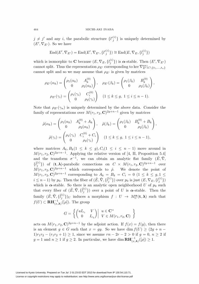
464 MICHI-AKI INABA
j �= j′ and any i, the parabolic structure {l′(i)j } is uniquely determined by
(E′,∇E′). So we have
End(E′,∇E′) = End(E′,∇E′ , {l′(i)j }) ∼= End(E,∇E, {l(i)j })
which is isomorphic to C because (E,∇E, {l(i)j }) is α-stable. Then (E′,∇E′)
cannot split. Thus the representation ρE′ corresponding to ker∇anE′ |C\{t1,...,tn}
cannot split and so we may assume that ρE′ is given by matrices
ρE′(αk) =
(ρ1(αk) A
(0)k
0 ρ2(αk)
), ρE′(βk) =
(ρ1(βk) B
(0)k
0 ρ2(βk)
),
ρE′(γi) =
(ρ1(γi) C
(0)i
0 ρ2(γi)
)(1 ≤ k ≤ g, 1 ≤ i ≤ n− 1).
Note that ρE′(γn) is uniquely determined by the above data. Consider the
family of representations over M(r1, r2,C)2g+n−1 given by matrices
ρ(αk) =
(ρ1(αk) A
(0)k +Ak
0 ρ2(αk)
), ρ(βk) =
(ρ1(βk) B
(0)k +Bk
0 ρ2(βk)
),
ρ(γi) =
(ρ1(γi) C
(0)i + Ci
0 ρ2(γi)
)(1 ≤ k ≤ g, 1 ≤ i ≤ n− 1),
where matrices Ak, Bk(1 ≤ k ≤ g), Ci(1 ≤ i ≤ n − 1) move around in
M(r1, r2,C)2g+n−1. Applying the relative version of [4, II, Proposition 5.4]
and the transform σ−1, we can obtain an analytic flat family (E, ∇,
{l(i)j }) of (t,λ)-parabolic connections on C × M(r1, r2,C)2g+n−1 over
M(r1, r2,C)2g+n−1 which corresponds to ρ. We denote the point of
M(r1, r2,C)2g+n−1 corresponding to Ak = Bk = Ci = 0 (1 ≤ k ≤ g, 1 ≤i ≤ n− 1) by p0. Then the fiber of (E, ∇, {l(i)j }) over p0 is just (E,∇E, {l(i)j })which is α-stable. So there is an analytic open neighborhood U of p0 such
that every fiber of (E, ∇, {l(i)j }) over a point of U is α-stable. Then the
family (E, ∇, {l(i)j })U induces a morphism f : U → MαC (t,λ) such that
f(U) ⊂ RH−1(x,λ)([ρ]). The group
G =
{(uIr1 V
0 Ir2
)∣∣∣∣ u ∈ C×
V ∈ M(r1, r2,C)
}
acts on M(r1, r2,C)2g+n−1 by the adjoint action. If f(x) = f(y), then there
is an element g ∈ G such that x = gy. So we have dim f(U) ≥ (2g + n −1)r1r2 − (r1r2 + 1) ≥ 1, since we assume rn − 2r − 2 > 0 if g = 0, n ≥ 2 if
g = 1 and n ≥ 1 if g ≥ 2. In particular, we have dimRH−1(x,λ)([ρ]) ≥ 1.
Licensed to Kyoto University. Prepared on Tue Jul 2 01:23:02 EDT 2013 for download from IP 130.54.110.71.
License or copyright restrictions may apply to redistribution; see http://www.ams.org/license/jour-dist-license.pdf
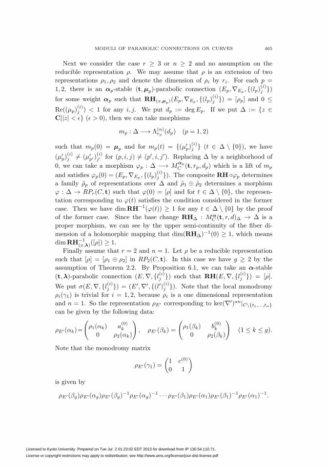
MODULI OF PARABOLIC CONNECTIONS ON CURVES 465
Next we consider the case r ≥ 3 or n ≥ 2 and no assumption on the
reducible representation ρ. We may assume that ρ is an extension of two
representations ρ1, ρ2 and denote the dimension of ρi by ri. For each p =
1, 2, there is an αp-stable (t,μp)-parabolic connection (Ep,∇Ep, {(lp)(i)j })
for some weight αp such that RH(x,μp)(Ep,∇Ep
, {(lp)(i)j }) = [ρp] and 0 ≤Re((μp)
(i)j ) < 1 for any i, j. We put dp := degEp. If we put Δ := {z ∈
C||z| < ε} (ε > 0), then we can take morphisms
mp : Δ −→ Λ(n)rp (dp) (p = 1, 2)
such that mp(0) = μp and for mp(t) = {(μ′p)
(i)j } (t ∈ Δ \ {0}), we have
(μ′p)
(i)j �= (μ′
p′)(i)j′ for (p, i, j) �= (p′, i, j′). Replacing Δ by a neighborhood of
0, we can take a morphism ϕp : Δ −→ Mαp
C (t, rp, dp) which is a lift of mp
and satisfies ϕp(0) = (Ep,∇Ep, {(lp)(i)j }). The composite RH ◦ϕp determines
a family ρp of representations over Δ and ρ1 ⊕ ρ2 determines a morphism
ϕ : Δ → RPr(C, t) such that ϕ(0) = [ρ] and for t ∈ Δ \ {0}, the represen-
tation corresponding to ϕ(t) satisfies the condition considered in the former
case. Then we have dimRH−1(ϕ(t)) ≥ 1 for any t ∈ Δ \ {0} by the proof
of the former case. Since the base change RHΔ : MαC (t, r, d)Δ → Δ is a
proper morphism, we can see by the upper semi-continuity of the fiber di-
mension of a holomorphic mapping that dim(RHΔ)−1(0) ≥ 1, which means
dimRH−1(x,λ)([ρ]) ≥ 1.
Finally assume that r = 2 and n = 1. Let ρ be a reducible representation
such that [ρ] = [ρ1 ⊕ ρ2] in RP2(C, t). In this case we have g ≥ 2 by the
assumption of Theorem 2.2. By Proposition 6.1, we can take an α-stable
(t,λ)-parabolic connection (E,∇, {l(i)j }) such that RH(E,∇, {l(i)j }) = [ρ].
We put σ(E,∇, {l(i)j }) = (E′,∇′, {(l′)(i)j }). Note that the local monodromy
ρi(γ1) is trivial for i = 1, 2, because ρi is a one dimensional representation
and n = 1. So the representation ρE′ corresponding to ker(∇′)an|C\{t1,...,tn}can be given by the following data:
ρE′(αk)=
(ρ1(αk) a
(0)k
0 ρ2(αk)
), ρE′(βk) =
(ρ1(βk) b
(0)k
0 ρ2(βk)
)(1 ≤ k ≤ g).
Note that the monodromy matrix
ρE′(γ1) =
(1 c(0)
0 1
)is given by
ρE′(βg)ρE′(αg)ρE′(βg)−1ρE′(αg)
−1 · · · ρE′(β1)ρE′(α1)ρE′(β1)−1ρE′(α1)
−1.
Licensed to Kyoto University. Prepared on Tue Jul 2 01:23:02 EDT 2013 for download from IP 130.54.110.71.
License or copyright restrictions may apply to redistribution; see http://www.ams.org/license/jour-dist-license.pdf
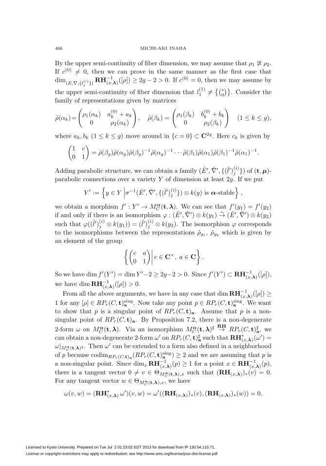
466 MICHI-AKI INABA
By the upper semi-continuity of fiber dimension, we may assume that ρ1 �∼= ρ2.
If c(0) �= 0, then we can prove in the same manner as the first case that
dim(E,∇,{l(i)j }) RH−1
(x,λ)([ρ]) ≥ 2g − 2 > 0. If c(0) = 0, then we may assume by
the upper semi-continuity of fiber dimension that l(1)1 �=
{(∗0
)}. Consider the
family of representations given by matrices
ρ(αk)=
(ρ1(αk) a
(0)k + ak
0 ρ2(αk)
), ρ(βk) =
(ρ1(βk) b
(0)k + bk
0 ρ2(βk)
)(1 ≤ k ≤ g),
where ak, bk (1 ≤ k ≤ g) move around in {c = 0} ⊂ C2g. Here ck is given by(1 c
0 1
)= ρ(βg)ρ(αg)ρ(βg)
−1ρ(αg)−1 · · · ρ(β1)ρ(α1)ρ(β1)
−1ρ(α1)−1.
Adding parabolic structure, we can obtain a family (E′, ∇′, {(l′)(i)j }) of (t,μ)-parabolic connections over a variety Y of dimension at least 2g. If we put
Y ′ :={y ∈ Y
∣∣∣σ−1(E′, ∇′, {(l′)(i)j })⊗ k(y) is α-stable},
we obtain a morphism f ′ : Y ′ → MαC (t,λ). We can see that f ′(y1) = f ′(y2)
if and only if there is an isomorphism ϕ : (E′, ∇′)⊗ k(y1)∼→ (E′, ∇′)⊗ k(y2)
such that ϕ((l′)(i)j ⊗ k(y1)) = (l′)
(i)j ⊗ k(y2). The isomorphism ϕ corresponds
to the isomorphisms between the representations ρy1, ρy2
which is given by
an element of the group{(c a
0 1
)∣∣∣∣ c ∈ C×, a ∈ C
}.
So we have dim f ′(Y ′) = dimY ′−2 ≥ 2g−2 > 0. Since f ′(Y ′) ⊂ RH−1(x,λ)([ρ]),
we have dimRH−1(x,λ)([ρ]) > 0.
From all the above arguments, we have in any case that dimRH−1(x,λ)([ρ]) ≥
1 for any [ρ] ∈ RPr(C, t)singa . Now take any point p ∈ RPr(C, t)
singa . We want
to show that p is a singular point of RPr(C, t)a. Assume that p is a non-
singular point of RPr(C, t)a. By Proposition 7.2, there is a non-degenerate
2-form ω on MαC (t,λ). Via an isomorphism Mα
C (t,λ)�RH→ RPr(C, t)
�a, we
can obtain a non-degenerate 2-form ω′ on RPr(C, t)�a such thatRH∗
(x,λ)(ω′) =
ω|MαC (t,λ)� . Then ω′ can be extended to a form also defined in a neighborhood
of p because codimRPr(C,t)a(RPr(C, t)singa ) ≥ 2 and we are assuming that p is
a non-singular point. Since dimx RH−1(x,λ)(p) ≥ 1 for a point x ∈ RH−1
(x,λ)(p),
there is a tangent vector 0 �= v ∈ ΘMαC (t,λ),x such that (RH(x,λ))∗(v) = 0.
For any tangent vector w ∈ ΘMαC (t,λ),x, we have
ω(v, w) = (RH∗(x,λ) ω
′)(v, w) = ω′((RH(x,λ))∗(v), (RH(x,λ))∗(w)) = 0.
Licensed to Kyoto University. Prepared on Tue Jul 2 01:23:02 EDT 2013 for download from IP 130.54.110.71.
License or copyright restrictions may apply to redistribution; see http://www.ams.org/license/jour-dist-license.pdf
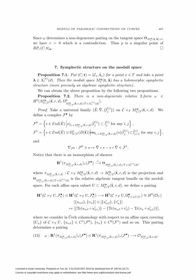
MODULI OF PARABOLIC CONNECTIONS ON CURVES 467
Since ω determines a non-degenerate pairing on the tangent space ΘMαC (t,λ),x,
we have v = 0 which is a contradiction. Thus p is a singular point of
RPr(C, t)a. �
7. Symplectic structure on the moduli space
Proposition 7.1. Put (C, t) = (Cx, tx) for a point x ∈ T and take a point
λ ∈ Λ(n)r (d). Then the moduli space Mα
C (t,λ) has a holomorphic symplectic
structure (more precisely an algebraic symplectic structure).
We can obtain the above proposition by the following two propositions.
Proposition 7.2. There is a non-degenerate relative 2-form ω ∈H0(Mα
C/T (t, r, d),Ω2
MαC/T
(t,r,d)/T×Λ(n)r (d)
).
Proof. Take a universal family (E, ∇, {l(i)j }) on C ×T MαC/T (t, r, d). We
define a complex F• by
F0 ={s ∈ End(E)
∣∣∣s|ti×MαC/T
(t,r,d)(l(i)j ) ⊂ l
(i)j for any i, j
},
F1 ={s ∈ End(E)⊗ Ω1
C/T (D(t))∣∣∣resti×Mα
C/T(t,r,d)(s)(l
(i)j )⊂ l
(i)j+1 for any i, j
},
and
∇F• : F0 � s �→ ∇ ◦ s− s ◦ ∇ ∈ F1.
Notice that there is an isomorphism of sheaves
R1(πMαC/T
(t,r,d))∗(F•)∼−→ Θ
MαC/T
(t,r,d)/T×Λ(n)r (d)
,
where πMαC/T
(t,r,d) : C ×T MαC/T (t, r, d) → Mα
C/T (t, r, d) is the projection and
ΘMα
C/T(t,r,d)/T×Λ
(n)r (d)
is the relative algebraic tangent bundle on the moduli
space. For each affine open subset U ⊂ MαC/T (t, r, d), we define a pairing
H1(C ×T U,F•U )⊗H1(C ×T U,F•
U ) −→ H2(C ×T U,Ω•C×TU/U )
∼= H0(OU )
[{uαβ}, {vα}]⊗ [{u′αβ}, {v′α}]
�→ [{Tr(uαβ ◦ u′βγ)} − {Tr(uαβ ◦ v′β)− Tr(vα ◦ u′
αβ)}],
where we consider in Cech cohomology with respect to an affine open covering
{Uα} of C ×T U , {uαβ} ∈ C1(F0), {vα} ∈ C0(F1) and so on. This pairing
determines a pairing
(13) ω : R1(πMαC/T
(t,r,d))∗(F•)⊗R1(πMαC/T
(t,r,d))∗(F•) −→ OMαC/T
(t,r,d).
Licensed to Kyoto University. Prepared on Tue Jul 2 01:23:02 EDT 2013 for download from IP 130.54.110.71.
License or copyright restrictions may apply to redistribution; see http://www.ams.org/license/jour-dist-license.pdf
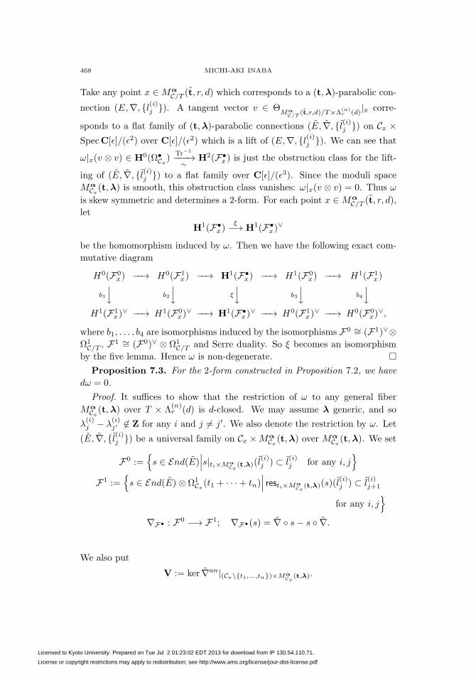
468 MICHI-AKI INABA
Take any point x ∈ MαC/T (t, r, d) which corresponds to a (t,λ)-parabolic con-
nection (E,∇, {l(i)j }). A tangent vector v ∈ ΘMα
C/T(t,r,d)/T×Λ
(n)r (d)
|x corre-
sponds to a flat family of (t,λ)-parabolic connections (E, ∇, {l(i)j }) on Cx ×SpecC[ε]/(ε2) over C[ε]/(ε2) which is a lift of (E,∇, {l(i)j }). We can see that
ω|x(v ⊗ v) ∈ H0(Ω•Cx)
Tr−1
−−−→∼
H2(F•x) is just the obstruction class for the lift-
ing of (E, ∇, {l(i)j }) to a flat family over C[ε]/(ε3). Since the moduli space
MαCx(t,λ) is smooth, this obstruction class vanishes: ω|x(v ⊗ v) = 0. Thus ω
is skew symmetric and determines a 2-form. For each point x ∈ MαC/T (t, r, d),
let
H1(F•x)
ξ−→ H1(F•x)
∨
be the homomorphism induced by ω. Then we have the following exact com-
mutative diagram
H0(F0x) −−→ H0(F1
x) −−→ H1(F•x) −−→ H1(F0
x) −−→ H1(F1x)
b1
⏐⏐� b2
⏐⏐� ξ
⏐⏐� b3
⏐⏐� b4
⏐⏐�H1(F1
x)∨ −−→ H1(F0
x)∨ −−→ H1(F•
x)∨ −−→ H0(F1
x)∨ −−→ H0(F0
x)∨,
where b1, . . . , b4 are isomorphisms induced by the isomorphisms F0 ∼= (F1)∨⊗Ω1
C/T , F1 ∼= (F0)∨ ⊗ Ω1C/T and Serre duality. So ξ becomes an isomorphism
by the five lemma. Hence ω is non-degenerate. �Proposition 7.3. For the 2-form constructed in Proposition 7.2, we have
dω = 0.
Proof. It suffices to show that the restriction of ω to any general fiber
MαCx(t,λ) over T × Λ
(n)r (d) is d-closed. We may assume λ generic, and so
λ(i)j − λ
(i)j′ �∈ Z for any i and j �= j′. We also denote the restriction by ω. Let
(E, ∇, {l(i)j }) be a universal family on Cx ×MαCx(t,λ) over Mα
Cx(t,λ). We set
F0 :={s ∈ End(E)
∣∣∣s|ti×MαCx
(t,λ)(l(i)j ) ⊂ l
(i)j for any i, j
}F1 :=
{s ∈ End(E)⊗ Ω1
Cx(t1 + · · ·+ tn)
∣∣∣ resti×MαCx
(t,λ)(s)(l(i)j ) ⊂ l
(i)j+1
for any i, j}
∇F• : F0 −→ F1; ∇F•(s) = ∇ ◦ s− s ◦ ∇.
We also put
V := ker ∇an|(Cx\{t1,...,tn})×MαCx
(t,λ).
Licensed to Kyoto University. Prepared on Tue Jul 2 01:23:02 EDT 2013 for download from IP 130.54.110.71.
License or copyright restrictions may apply to redistribution; see http://www.ams.org/license/jour-dist-license.pdf
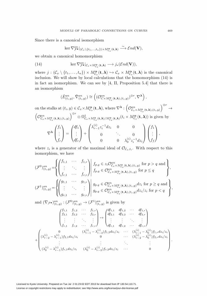
MODULI OF PARABOLIC CONNECTIONS ON CURVES 469
Since there is a canonical isomorphism
ker∇anF• |(Cx\{t1,...,tn})×Mα
Cx(t,λ)
∼−→ End(V),
we obtain a canonical homomorphism
(14) ker∇anF• |Cx×Mα
Cx(t,λ) −→ j∗(End(V)),
where j : (Cx \ {t1, . . . , tn}) × MαCx(t,λ) ↪→ Cx × Mα
Cx(t,λ) is the canonical
inclusion. We will show by local calculations that the homomorphism (14) is
in fact an isomorphism. We can see by [4, II, Proposition 5.4] that there is
an isomorphism
(Ean(ti,y)
, ∇an(ti,y)
) ∼=((Oan
C×MαCx
(t,λ),(ti,y))⊕r,∇λ
),
on the stalks at (ti, y) ∈ Cx×MαCx(t,λ), where∇λ :
(Oan
Cx×MαCx
(t,λ),(ti,y)
)⊕r
→(Oan
Cx×MαCx
(t,λ),(ti,y)
)⊕r
⊗ Ω1Cx×Mα
Cx(t,λ)/Mα
Cx(t,λ)(ti ×Mα
Cx(t,λ)) is given by
∇λ
⎛⎜⎝f1...
fr
⎞⎟⎠ =
⎛⎜⎝df1...
dfr
⎞⎟⎠+
⎛⎜⎜⎝λ(i)r−1z
−1i dzi 0 0
0. . . 0
0 0 λ(i)0 z−1
i dzi
⎞⎟⎟⎠⎛⎜⎝f1...
ff
⎞⎟⎠ ,
where zi is a generator of the maximal ideal of OCx,ti . With respect to this
isomorphism, we have
(F0)an(ti,y)=
⎧⎪⎨⎪⎩⎛⎜⎝f1,1 · · · f1,r...
. . ....
fr,1 · · · fr,r
⎞⎟⎠∣∣∣∣∣∣∣fp,q ∈ ziOan
Cx×MαCx
(t,λ),(ti,y)for p > q and
fp,q ∈ OanCx×Mα
Cx(t,λ),(ti,y)
for p ≤ q
⎫⎪⎬⎪⎭,
(F1)an(ti,y)=
⎧⎪⎨⎪⎩⎛⎜⎝g1,1 · · · g1,r...
. . ....
gr,1 · · · gr,r
⎞⎟⎠∣∣∣∣∣∣∣gp,q ∈ Oan
Cx×MαCx
(t,λ),(ti,y)dzi for p ≥ q and
gp,q ∈ OanCx×Mα
Cx(t,λ),(ti,y)
dzi/zi for p < q
⎫⎪⎬⎪⎭,
and (∇F•)an(ti,y) : (F0)an(ti,y) → (F1)an(ti,y) is given by
⎛⎜⎜⎜⎝
f1,1 f1,2 · · · f1,rf2,1 f2,2 · · · f2,r...
..
.. . .
..
.fr,1 fr,2 · · · fr,r
⎞⎟⎟⎟⎠ �→
⎛⎜⎜⎜⎝
df1,1 df1,2 · · · df1,rdf2,1 df2,2 · · · df2,r...
..
.. . .
..
.dfr,1 dfr,2 · · · dfr,r
⎞⎟⎟⎟⎠
+
⎛⎜⎜⎜⎜⎜⎝
0 (λ(i)r−1 − λ
(i)r−2)f1,2dzi/zi · · · (λ
(i)r−1 − λ
(i)0 )f1,rdzi/zi
(λ(i)r−2 − λ
(i)r−1)f2,1dzi/zi 0 · · · (λ
(i)r−2 − λ
(i)0 )f2,rdzi/zi
.
.....
. . ....
(λ(i)0 − λ
(i)r−1)fr,1dzi/zi (λ
(i)0 − λ
(i)r−2)fr,2dzi/zi · · · 0
⎞⎟⎟⎟⎟⎟⎠
.
Licensed to Kyoto University. Prepared on Tue Jul 2 01:23:02 EDT 2013 for download from IP 130.54.110.71.
License or copyright restrictions may apply to redistribution; see http://www.ams.org/license/jour-dist-license.pdf
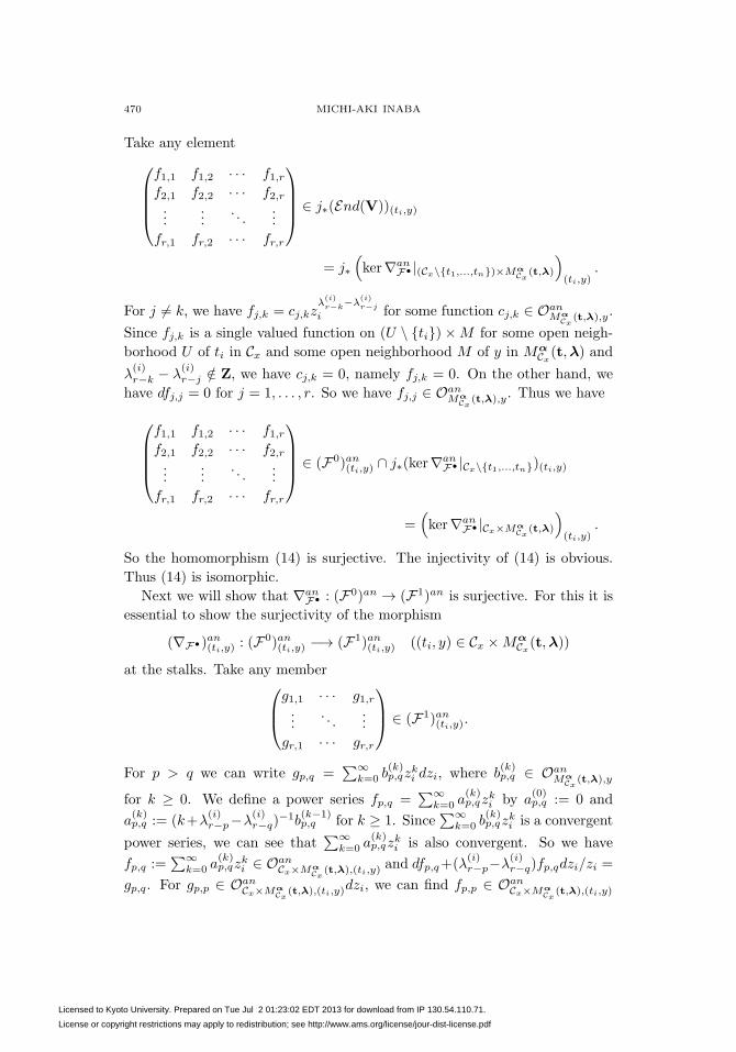
470 MICHI-AKI INABA
Take any element⎛⎜⎜⎜⎝f1,1 f1,2 · · · f1,rf2,1 f2,2 · · · f2,r...
.... . .
...
fr,1 fr,2 · · · fr,r
⎞⎟⎟⎟⎠ ∈ j∗(End(V))(ti,y)
= j∗(ker∇an
F• |(Cx\{t1,...,tn})×MαCx
(t,λ)
)(ti,y)
.
For j �= k, we have fj,k = cj,kzλ(i)r−k−λ
(i)r−j
i for some function cj,k ∈ OanMα
Cx(t,λ),y.
Since fj,k is a single valued function on (U \ {ti})×M for some open neigh-
borhood U of ti in Cx and some open neighborhood M of y in MαCx(t,λ) and
λ(i)r−k − λ
(i)r−j /∈ Z, we have cj,k = 0, namely fj,k = 0. On the other hand, we
have dfj,j = 0 for j = 1, . . . , r. So we have fj,j ∈ OanMα
Cx(t,λ),y. Thus we have
⎛⎜⎜⎜⎝f1,1 f1,2 · · · f1,rf2,1 f2,2 · · · f2,r...
.... . .
...
fr,1 fr,2 · · · fr,r
⎞⎟⎟⎟⎠ ∈ (F0)an(ti,y) ∩ j∗(ker∇an
F• |Cx\{t1,...,tn})(ti,y)
=(ker∇an
F• |Cx×MαCx
(t,λ)
)(ti,y)
.
So the homomorphism (14) is surjective. The injectivity of (14) is obvious.
Thus (14) is isomorphic.
Next we will show that ∇anF• : (F0)an → (F1)an is surjective. For this it is
essential to show the surjectivity of the morphism
(∇F•)an(ti,y) : (F0)an(ti,y) −→ (F1)an(ti,y) ((ti, y) ∈ Cx ×Mα
Cx(t,λ))
at the stalks. Take any member⎛⎜⎝g1,1 · · · g1,r...
. . ....
gr,1 · · · gr,r
⎞⎟⎠ ∈ (F1)an(ti,y).
For p > q we can write gp,q =∑∞
k=0 b(k)p,qzki dzi, where b
(k)p,q ∈ Oan
MαCx
(t,λ),y
for k ≥ 0. We define a power series fp,q =∑∞
k=0 a(k)p,qzki by a
(0)p,q := 0 and
a(k)p,q := (k+λ
(i)r−p−λ
(i)r−q)
−1b(k−1)p,q for k ≥ 1. Since
∑∞k=0 b
(k)p,qzki is a convergent
power series, we can see that∑∞
k=0 a(k)p,qzki is also convergent. So we have
fp,q :=∑∞
k=0 a(k)p,qzki ∈ Oan
Cx×MαCx
(t,λ),(ti,y)and dfp,q+(λ
(i)r−p−λ
(i)r−q)fp,qdzi/zi =
gp,q. For gp,p ∈ OanCx×Mα
Cx(t,λ),(ti,y)
dzi, we can find fp,p ∈ OanCx×Mα
Cx(t,λ),(ti,y)
Licensed to Kyoto University. Prepared on Tue Jul 2 01:23:02 EDT 2013 for download from IP 130.54.110.71.
License or copyright restrictions may apply to redistribution; see http://www.ams.org/license/jour-dist-license.pdf
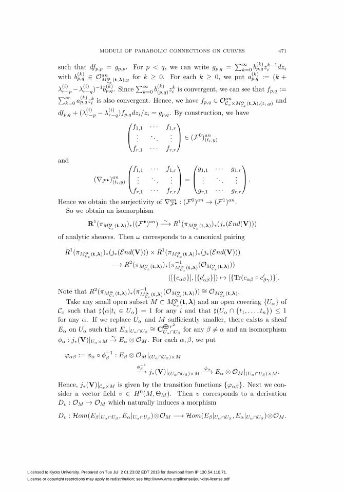
MODULI OF PARABOLIC CONNECTIONS ON CURVES 471
such that dfp,p = gp,p. For p < q, we can write gp,q =∑∞
k=0 b(k)p,qz
k−1i dzi
with b(k)p,q ∈ Oan
MαCx
(t,λ),y for k ≥ 0. For each k ≥ 0, we put a(k)p,q := (k +
λ(i)r−p−λ
(i)r−q)
−1b(k)p,q . Since
∑∞k=0 b
(k)(p,q)z
ki is convergent, we can see that fp,q :=∑∞
k=0 a(k)p,qzki is also convergent. Hence, we have fp,q ∈ Oan
Cx×MαCx
(t,λ),(ti,y)and
dfp,q + (λ(i)r−p − λ
(i)r−q)fp,qdzi/zi = gp,q . By construction, we have⎛
⎜⎝f1,1 · · · f1,r...
. . ....
fr,1 · · · fr,r
⎞⎟⎠ ∈ (F0)an(ti,y)
and
(∇F•)an(ti,y)
⎛⎜⎝f1,1 · · · f1,r...
. . ....
fr,1 · · · fr,r
⎞⎟⎠ =
⎛⎜⎝g1,1 · · · g1,r...
. . ....
gr,1 · · · gr,r
⎞⎟⎠ .
Hence we obtain the surjectivity of ∇anF• : (F0)an → (F1)an.
So we obtain an isomorphism
R1(πMαCx
(t,λ))∗((F•)an)∼−→ R1(πMα
Cx(t,λ))∗(j∗(End(V)))
of analytic sheaves. Then ω corresponds to a canonical pairing
R1(πMαCx
(t,λ))∗(j∗(End(V)))×R1(πMαCx
(t,λ))∗(j∗(End(V)))
−→ R2(πMαCx
(t,λ))∗(π−1Mα
Cx(t,λ)(OMα
Cx(t,λ)))
([{cαβ}], [{c′αβ}]) �→ [{Tr(cαβ ◦ c′βγ)}].
Note that R2(πMαCx
(t,λ))∗(π−1Mα
Cx(t,λ)(OMα
Cx(t,λ))) ∼= OMα
Cx(t,λ).
Take any small open subset M ⊂ MαCx(t,λ) and an open covering {Uα} of
Cx such that �{α|ti ∈ Uα} = 1 for any i and that �(Uα ∩ {t1, . . . , tn}) ≤ 1
for any α. If we replace Uα and M sufficiently smaller, there exists a sheaf
Eα on Uα such that Eα|Uα∩Uβ∼= C
⊕r2
Uα∩Uβfor any β �= α and an isomorphism
φα : j∗(V)|Uα×M∼→ Eα ⊗OM . For each α, β, we put
ϕαβ := φα ◦ φ−1β : Eβ ⊗OM |(Uα∩Uβ)×M
φ−1β−→ j∗(V)|(Uα∩Uβ)×M
φα−→ Eα ⊗OM |(Uα∩Uβ)×M .
Hence, j∗(V)|Cx×M is given by the transition functions {ϕαβ}. Next we con-
sider a vector field v ∈ H0(M,ΘM ). Then v corresponds to a derivation
Dv : OM → OM which naturally induces a morphism
Dv : Hom(Eβ|Uα∩Uβ, Eα|Uα∩Uβ
)⊗OM −→ Hom(Eβ|Uα∩Uβ, Eα|Uα∩Uβ
)⊗OM .
Licensed to Kyoto University. Prepared on Tue Jul 2 01:23:02 EDT 2013 for download from IP 130.54.110.71.
License or copyright restrictions may apply to redistribution; see http://www.ams.org/license/jour-dist-license.pdf
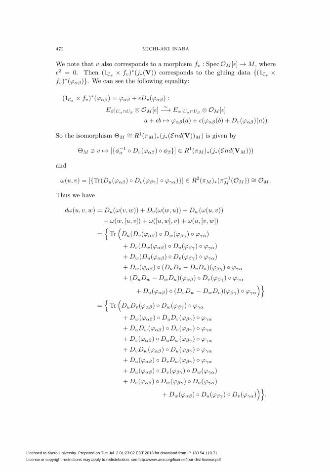
472 MICHI-AKI INABA
We note that v also corresponds to a morphism fv : SpecOM [ε] → M , where
ε2 = 0. Then (1Cx× fv)
∗(j∗(V)) corresponds to the gluing data {(1Cx×
fv)∗(ϕαβ)}. We can see the following equality:
(1Cx× fv)
∗(ϕαβ) = ϕαβ + εDv(ϕαβ) :
Eβ|Uα∩Uβ⊗OM [ε]
∼−→ Eα|Uα∩Uβ⊗OM [ε]
a+ εb �→ ϕαβ(a) + ε(ϕαβ(b) +Dv(ϕαβ)(a)).
So the isomorphism ΘM∼= R1(πM )∗(j∗(End(V))M ) is given by
ΘM � v �→ [{φ−1α ◦Dv(ϕαβ) ◦ φβ}] ∈ R1(πM )∗(j∗(End(VM )))
and
ω(u, v) = [{Tr(Du(ϕαβ) ◦Dv(ϕβγ) ◦ ϕγα)}] ∈ R2(πM )∗(π−1M (OM )) ∼= OM .
Thus we have
dω(u, v, w) = Du(ω(v, w)) +Dv(ω(w, u)) +Dw(ω(u, v))
+ ω(w, [u, v]) + ω([u,w], v) + ω(u, [v, w])
={Tr(Du(Dv(ϕαβ) ◦Dw(ϕβγ) ◦ ϕγα)
+Dv(Dw(ϕαβ) ◦Du(ϕβγ) ◦ ϕγα)
+Dw(Du(ϕαβ) ◦Dv(ϕβγ) ◦ ϕγα)
+Dw(ϕαβ) ◦ (DuDv −DvDu)(ϕβγ) ◦ ϕγα
+ (DuDw −DwDu)(ϕαβ) ◦Dv(ϕβγ) ◦ ϕγα
+Du(ϕαβ) ◦ (DvDw −DwDv)(ϕβγ) ◦ ϕγα
)}={Tr(DuDv(ϕαβ) ◦Dw(ϕβγ) ◦ ϕγα
+Dw(ϕαβ) ◦DuDv(ϕβγ) ◦ ϕγα
+DuDw(ϕαβ) ◦Dv(ϕβγ) ◦ ϕγα
+Dv(ϕαβ) ◦DuDw(ϕβγ) ◦ ϕγα
+DvDw(ϕαβ) ◦Du(ϕβγ) ◦ ϕγα
+Du(ϕαβ) ◦DvDw(ϕβγ) ◦ ϕγα
+Du(ϕαβ) ◦Dv(ϕβγ) ◦Dw(ϕγα)
+Dv(ϕαβ) ◦Dw(ϕβγ) ◦Du(ϕγα)
+Dw(ϕαβ) ◦Du(ϕβγ) ◦Dv(ϕγα))}
.
Licensed to Kyoto University. Prepared on Tue Jul 2 01:23:02 EDT 2013 for download from IP 130.54.110.71.
License or copyright restrictions may apply to redistribution; see http://www.ams.org/license/jour-dist-license.pdf
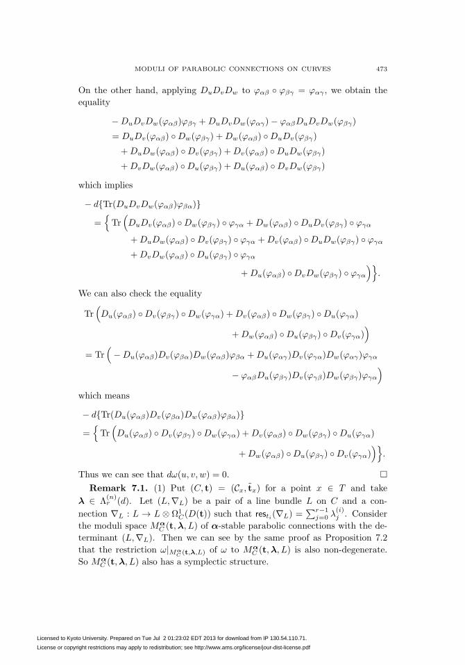
MODULI OF PARABOLIC CONNECTIONS ON CURVES 473
On the other hand, applying DuDvDw to ϕαβ ◦ ϕβγ = ϕαγ , we obtain the
equality
−DuDvDw(ϕαβ)ϕβγ +DuDvDw(ϕαγ)− ϕαβDuDvDw(ϕβγ)
= DuDv(ϕαβ) ◦Dw(ϕβγ) +Dw(ϕαβ) ◦DuDv(ϕβγ)
+DuDw(ϕαβ) ◦Dv(ϕβγ) +Dv(ϕαβ) ◦DuDw(ϕβγ)
+DvDw(ϕαβ) ◦Du(ϕβγ) +Du(ϕαβ) ◦DvDw(ϕβγ)
which implies
− d{Tr(DuDvDw(ϕαβ)ϕβα)}
={Tr(DuDv(ϕαβ) ◦Dw(ϕβγ) ◦ ϕγα +Dw(ϕαβ) ◦DuDv(ϕβγ) ◦ ϕγα
+DuDw(ϕαβ) ◦Dv(ϕβγ) ◦ ϕγα +Dv(ϕαβ) ◦DuDw(ϕβγ) ◦ ϕγα
+DvDw(ϕαβ) ◦Du(ϕβγ) ◦ ϕγα
+Du(ϕαβ) ◦DvDw(ϕβγ) ◦ ϕγα
)}.
We can also check the equality
Tr(Du(ϕαβ) ◦Dv(ϕβγ) ◦Dw(ϕγα) +Dv(ϕαβ) ◦Dw(ϕβγ) ◦Du(ϕγα)
+Dw(ϕαβ) ◦Du(ϕβγ) ◦Dv(ϕγα))
= Tr(−Du(ϕαβ)Dv(ϕβα)Dw(ϕαβ)ϕβα +Du(ϕαγ)Dv(ϕγα)Dw(ϕαγ)ϕγα
− ϕαβDu(ϕβγ)Dv(ϕγβ)Dw(ϕβγ)ϕγα
)which means
− d{Tr(Du(ϕαβ)Dv(ϕβα)Dw(ϕαβ)ϕβα)}
={Tr(Du(ϕαβ) ◦Dv(ϕβγ) ◦Dw(ϕγα) +Dv(ϕαβ) ◦Dw(ϕβγ) ◦Du(ϕγα)
+Dw(ϕαβ) ◦Du(ϕβγ) ◦Dv(ϕγα))}
.
Thus we can see that dω(u, v, w) = 0. �Remark 7.1. (1) Put (C, t) = (Cx, tx) for a point x ∈ T and take
λ ∈ Λ(n)r (d). Let (L,∇L) be a pair of a line bundle L on C and a con-
nection ∇L : L → L ⊗ Ω1C(D(t)) such that resti(∇L) =
∑r−1j=0 λ
(i)j . Consider
the moduli space MαC (t,λ, L) of α-stable parabolic connections with the de-
terminant (L,∇L). Then we can see by the same proof as Proposition 7.2
that the restriction ω|MαC (t,λ,L) of ω to Mα
C (t,λ, L) is also non-degenerate.
So MαC (t,λ, L) also has a symplectic structure.
Licensed to Kyoto University. Prepared on Tue Jul 2 01:23:02 EDT 2013 for download from IP 130.54.110.71.
License or copyright restrictions may apply to redistribution; see http://www.ams.org/license/jour-dist-license.pdf

474 MICHI-AKI INABA
(2) By Proposition 8.1, we obtain a splitting ΘMα
C/T(t,r,d)/Λ
(n)r (d)
∼= π∗ΘT ⊕Θ
MαC/T
(t,r,d)/T×Λ(n)r (d)
. With respect to this splitting, we can lift ω to ω ∈H0(Ω2
MαC/T
(t,r,d)/Λ(n)r (d)
) and we have dω = 0. This 2-form ω is nothing but
the 2-form considered in [10] and [11]. Note that we have ω · v = 0 for
v ∈ D(π∗ΘT ), where D is the homomorphism given in Proposition 8.1.
8. Isomonodromic deformation
Let T → T be a universal covering. Then RPr(C, t)×T T → T becomes a
trivial fibration and we can consider the set of constant sections
F�R =
{σ : T → RPr(C, t)� ×T T
},
where
RPr(C, t)� =∐
(x,a)∈T×A(n)r
RPr(Cx, tx)�a.
The pull back F�M = {RH−1(σ)} of these constant sections determines a
foliation on MαC/T (t, r, d)
� ×T T where MαC/T (t, r, d)
� = RH−1(RPr(C, t)�).This foliation corresponds to a subbundle determined by a splitting
D� : π∗(ΘanT) → Θan
MαC/T
(t,r,d)�×T T
of the analytic tangent map
ΘanMα
C/T(t,r,d)�×T T
−→ π∗ΘanT
→ 0,
where π : MαC/T (t, r, d)
� ×T T → T is the projection. We will show that this
splitting D� is in fact induced by a splitting
D : π∗(ΘT ) → ΘMαC/T
(t,r,d)
of the algebraic tangent bundle, where π : MαC/T (t, r, d) → T is the projec-
tion. This splitting is nothing but the differential equation determined by the
isomonodromic deformation.
Usually, the equation of the isomonodromic deformation is given by the fol-
lowing way: Assume C = P1 and take a Zariski open set U ⊂ MαP1×T/T (t, r, 0)
such that a universal family on P1 × U is given by (O⊕rP1×U ,∇, {l(i)j }), where
∇ is given by a connection matrix
n∑i=1
Aidz
z − ti(Ai = (a
(i)jk )1≤j,k≤r ∈ Mr(OU )).
Licensed to Kyoto University. Prepared on Tue Jul 2 01:23:02 EDT 2013 for download from IP 130.54.110.71.
License or copyright restrictions may apply to redistribution; see http://www.ams.org/license/jour-dist-license.pdf
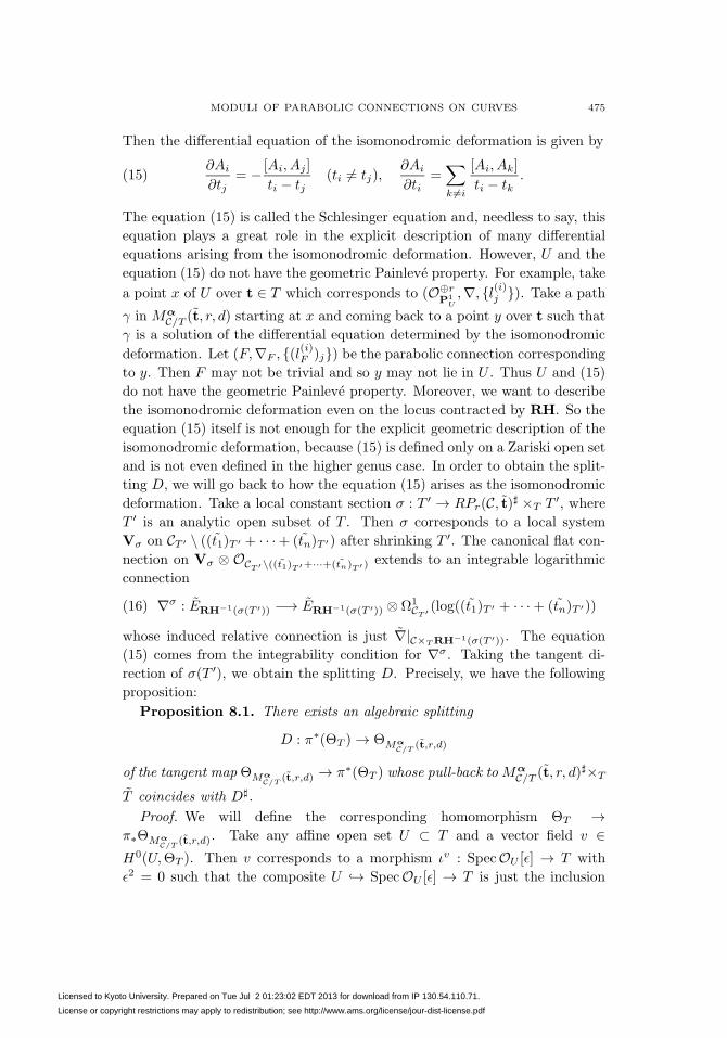
MODULI OF PARABOLIC CONNECTIONS ON CURVES 475
Then the differential equation of the isomonodromic deformation is given by
(15)∂Ai
∂tj= − [Ai, Aj ]
ti − tj(ti �= tj),
∂Ai
∂ti=∑k �=i
[Ai, Ak]
ti − tk.
The equation (15) is called the Schlesinger equation and, needless to say, this
equation plays a great role in the explicit description of many differential
equations arising from the isomonodromic deformation. However, U and the
equation (15) do not have the geometric Painleve property. For example, take
a point x of U over t ∈ T which corresponds to (O⊕rP1
U,∇, {l(i)j }). Take a path
γ in MαC/T (t, r, d) starting at x and coming back to a point y over t such that
γ is a solution of the differential equation determined by the isomonodromic
deformation. Let (F,∇F , {(l(i)F )j}) be the parabolic connection corresponding
to y. Then F may not be trivial and so y may not lie in U . Thus U and (15)
do not have the geometric Painleve property. Moreover, we want to describe
the isomonodromic deformation even on the locus contracted by RH. So the
equation (15) itself is not enough for the explicit geometric description of the
isomonodromic deformation, because (15) is defined only on a Zariski open set
and is not even defined in the higher genus case. In order to obtain the split-
ting D, we will go back to how the equation (15) arises as the isomonodromic
deformation. Take a local constant section σ : T ′ → RPr(C, t)� ×T T ′, where
T ′ is an analytic open subset of T . Then σ corresponds to a local system
Vσ on CT ′ \ ((t1)T ′ + · · ·+ (tn)T ′) after shrinking T ′. The canonical flat con-
nection on Vσ ⊗ OCT ′\((t1)T ′+···+(tn)T ′ ) extends to an integrable logarithmic
connection
(16) ∇σ : ERH−1(σ(T ′)) −→ ERH−1(σ(T ′)) ⊗ Ω1CT ′ (log((t1)T ′ + · · ·+ (tn)T ′))
whose induced relative connection is just ∇|C×TRH−1(σ(T ′)). The equation
(15) comes from the integrability condition for ∇σ. Taking the tangent di-
rection of σ(T ′), we obtain the splitting D. Precisely, we have the following
proposition:
Proposition 8.1. There exists an algebraic splitting
D : π∗(ΘT ) → ΘMαC/T
(t,r,d)
of the tangent map ΘMαC/T
(t,r,d) → π∗(ΘT ) whose pull-back to MαC/T (t, r, d)
�×T
T coincides with D�.
Proof. We will define the corresponding homomorphism ΘT →π∗ΘMα
C/T(t,r,d). Take any affine open set U ⊂ T and a vector field v ∈
H0(U,ΘT ). Then v corresponds to a morphism ιv : SpecOU [ε] → T with
ε2 = 0 such that the composite U ↪→ SpecOU [ε] → T is just the inclusion
Licensed to Kyoto University. Prepared on Tue Jul 2 01:23:02 EDT 2013 for download from IP 130.54.110.71.
License or copyright restrictions may apply to redistribution; see http://www.ams.org/license/jour-dist-license.pdf
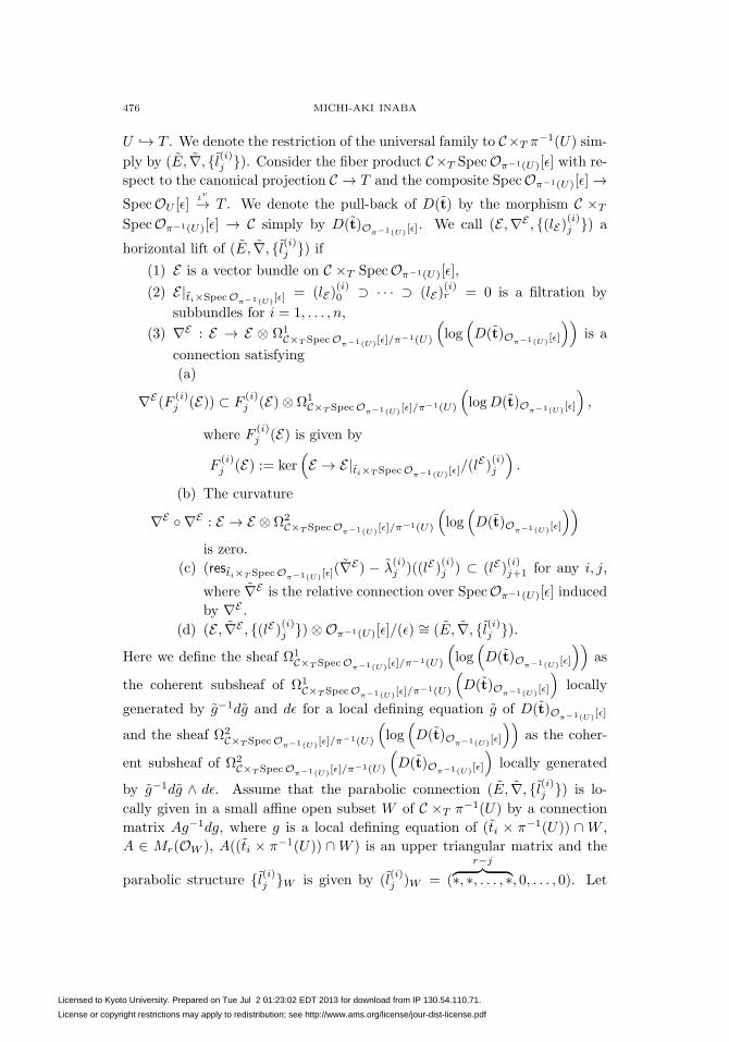
476 MICHI-AKI INABA
U ↪→ T . We denote the restriction of the universal family to C×T π−1(U) sim-
ply by (E, ∇, {l(i)j }). Consider the fiber product C×T SpecOπ−1(U)[ε] with re-
spect to the canonical projection C → T and the composite SpecOπ−1(U)[ε] →SpecOU [ε]
ιv→ T . We denote the pull-back of D(t) by the morphism C ×T
SpecOπ−1(U)[ε] → C simply by D(t)Oπ−1(U)[ε]. We call (E ,∇E , {(lE)(i)j }) a
horizontal lift of (E, ∇, {l(i)j }) if(1) E is a vector bundle on C ×T SpecOπ−1(U)[ε],
(2) E|ti×SpecOπ−1(U)[ε]= (lE)
(i)0 ⊃ · · · ⊃ (lE)
(i)r = 0 is a filtration by
subbundles for i = 1, . . . , n,
(3) ∇E : E → E ⊗ Ω1C×T SpecOπ−1(U)[ε]/π
−1(U)
(log(D(t)Oπ−1(U)[ε]
))is a
connection satisfying
(a)
∇E(F(i)j (E)) ⊂ F
(i)j (E)⊗ Ω1
C×TSpecOπ−1(U)[ε]/π−1(U)
(logD(t)Oπ−1(U)[ε]
),
where F(i)j (E) is given by
F(i)j (E) := ker
(E → E|ti×TSpecOπ−1(U)[ε]
/(lE)(i)j
).
(b) The curvature
∇E ◦ ∇E : E → E ⊗ Ω2C×TSpecOπ−1(U)[ε]/π
−1(U)
(log(D(t)Oπ−1(U)[ε]
))is zero.
(c) (resti×T SpecOπ−1(U)[ε](∇E) − λ
(i)j )((lE)
(i)j ) ⊂ (lE)
(i)j+1 for any i, j,
where ∇E is the relative connection over SpecOπ−1(U)[ε] induced
by ∇E .
(d) (E , ∇E , {(lE)(i)j })⊗Oπ−1(U)[ε]/(ε) ∼= (E, ∇, {l(i)j }).
Here we define the sheaf Ω1C×T SpecOπ−1(U)[ε]/π
−1(U)
(log(D(t)Oπ−1(U)[ε]
))as
the coherent subsheaf of Ω1C×T SpecOπ−1(U)[ε]/π
−1(U)
(D(t)Oπ−1(U)[ε]
)locally
generated by g−1dg and dε for a local defining equation g of D(t)Oπ−1(U)[ε]
and the sheaf Ω2C×TSpecOπ−1(U)[ε]/π
−1(U)
(log(D(t)Oπ−1(U)[ε]
))as the coher-
ent subsheaf of Ω2C×TSpecOπ−1(U)[ε]/π
−1(U)
(D(t)Oπ−1(U)[ε]
)locally generated
by g−1dg ∧ dε. Assume that the parabolic connection (E, ∇, {l(i)j }) is lo-
cally given in a small affine open subset W of C ×T π−1(U) by a connection
matrix Ag−1dg, where g is a local defining equation of (ti × π−1(U)) ∩ W ,
A ∈ Mr(OW ), A((ti × π−1(U)) ∩W ) is an upper triangular matrix and the
parabolic structure {l(i)j }W is given by (l(i)j )W = (
r−j︷ ︸︸ ︷∗, ∗, . . . , ∗, 0, . . . , 0). Let
Licensed to Kyoto University. Prepared on Tue Jul 2 01:23:02 EDT 2013 for download from IP 130.54.110.71.
License or copyright restrictions may apply to redistribution; see http://www.ams.org/license/jour-dist-license.pdf
MODULI OF PARABOLIC CONNECTIONS ON CURVES 477
W be the affine open subscheme of C × SpecOπ−1(U)[ε] whose underlying
space is W and let g be a lift of g which is a local defining equation of
(ti × SpecOπ−1(U)[ε]) ∩ W . If we denote the composite OWd→ Ω1
W/π−1(U)=
OW dg ⊕ OW dε → OW dε by dε, we can take a lift A ∈ Mr(OW ) of A such
that dε(A) = 0 and A((ti × SpecOπ−1(U)[ε]) ∩ W ) is an upper-triangular
matrix. Then the connection matrix Ag−1dg gives a local horizontal lift of
(E, ∇, {l(i)j })|W . We put
F0 :={u ∈ End(E)
∣∣∣u|ti×π−1(U)(l(i)j ) ⊂ l
(i)j (1 ≤ i ≤ n, 0 ≤ j ≤ r)
},
F1 :=
⎧⎪⎪⎪⎨⎪⎪⎪⎩u ∈ End(E)⊗ Ω1
∣∣∣∣∣∣∣∣∣u(F
(i)j (E)) ⊂ F
(i)j (E)⊗ Ω1
for any i, j and the image of
F(i)j (E)
u→ E ⊗ Ω1resti→ E|ti×π−1(U)
is contained in l(i)j+1 for any i, j
⎫⎪⎪⎪⎬⎪⎪⎪⎭ ,
F2 :={u ∈ End(E)⊗ Ω2
∣∣∣u(F (i)j (E)) ⊂ F
(i)j+1(E)⊗ Ω2 for any i, j
},
where we put
Ω1 := Ω1C×Tπ−1(U)/π−1(U)(D(t))⊕OC×Tπ−1(U)dε,
Ω2 := Ω1C×Tπ−1(U)/π−1(U)(D(t)) ∧ dε,
F(i)j (E) := ker
(E → E|ti×π−1(U)/l
(i)j
).
Consider the complex
F0 d0
−→ F1 d1
−→ F2
defined by d0(u) = ∇◦u−u◦∇+udε and d1(ω+adε) = dε∧ω+(∇◦a−a◦∇)∧dεfor u ∈ F0, ω ∈ End(E)⊗ g−1dg and a ∈ F0 such that ω + adε ∈ F1.
We can see that an obstruction class for the existence of a horizontal lift
of (E, ∇, {li}) is in H2(F•) and the set of horizontal lifts is isomorphic to
H1(F•) if it is not empty. It is obvious that d0 is injective and d1 is surjective.
Take any member ω + adε ∈ ker(d1). Then we have d1(ω + adε) = dε ∧ ω +
(∇ ◦ a − a ◦ ∇) ∧ dε = 0. So we have ω = ∇ ◦ a − a ◦ ∇ and d0(a) =
∇ ◦ a − a ◦ ∇ + adε = ω + adε. Thus F• is exact at F1. Hence F• is
an exact complex. Thus we have H2(F•) = 0, H1(F•) = 0 and there is
a unique horizontal lift (E ,∇E , {(lE)(i)j }) of (E, ∇, {li}). We can check that
v �→ (E , ∇E , {(lE)(i)j }) gives an OT -homomorphism ΘT → π∗(ΘMαC/T
(t,r,d)).
Thus we obtain an OMαC/T
(t,r,d)-homomorphism
D : π∗(ΘT ) → ΘMαC/T
(t,r,d)
Licensed to Kyoto University. Prepared on Tue Jul 2 01:23:02 EDT 2013 for download from IP 130.54.110.71.
License or copyright restrictions may apply to redistribution; see http://www.ams.org/license/jour-dist-license.pdf
478 MICHI-AKI INABA
which is a splitting of the surjection ΘMαC/T
(t,r,d) → π∗(ΘT ). By construction
we can see that the pull-back of D to MαC/T (t, r, d)
�× T coincides with D�. �
Remark 8.1. (1) We can see by construction that the image D(π∗ΘT ) is
in fact contained in the relative tangent bundle ΘMα
C/T(t,r,d)/Λ
(n)r (d)
.
(2) As is explained in section 2, the subbundle D(π∗ΘT ) ⊂ ΘMαC/T
(t,r,d) sat-
isfies an integrability condition and determines a foliation FM onMαC/T (t, r, d).
By the proof of Proposition 8.1, we can see that {RH(L)|L ∈ FM} coincides
with FR.
Proof of Theorem 2.3. Take any path γ : [0, 1] → T and a point x ∈Mα
C/T (t, r, d) such that π(x) = γ(0). We take a lift x ∈ MαC/T (t, r, d)×T T of
x. We can easily lift γ to a path γ : [0, 1] → (RPr(C, t) ×T T ) ×A(n)r
Λ(n)r (d)
such that γ[0, 1] is contained in a leaf of FR×A(n)r
Λ(n)r (d) and RH(x) = γ(0).
Since a leaf of FM passing through x is locally isomorphic to T , we can take
a unique local lift δε : [0, ε) → MαC/T (t, r, d) ×T T of γ for small ε > 0 such
that δε(0) = x and δε([0, ε]) is contained in a leaf of FM . Consider the set
A :=
⎧⎪⎨⎪⎩t ∈ (0, 1]
∣∣∣∣∣∣∣there exists a lift δt : [0, t) → Mα
C/T (t, r, d)×T T
of γ|[0,t) such that δ(0) = x and δ([0, t)) is contained
in a leaf of FM
⎫⎪⎬⎪⎭
and put a := supA. Assume that a < 1. Then there is a sequence {tn}n≥0 in
A such that limn→∞ tn = a. Since RH : MαC/T (t, r, d)×T T → (RPr(C, t)×T
T )×A(n)r
Λ(n)r (d) is a proper morphism, RH−1(γ[0, a]) is compact. Thus the se-
quence {δtn(tn)} in RH−1(γ[0, a]) has a subsequence {δtnk(tnk
)} which is con-
vergent in RH−1(γ[0, a]). We put xa := limk→∞ δtnk(tnk
) ∈ RH−1(γ[0, a]).
Then RH(xa) = γ(a) and we can take a local lift δa : (a − ε, a + ε) →Mα
C/T (t, r, d) ×T T of γ|(a−ε,a+ε) for small ε > 0 such that δa(a) = xa and
δa((a − ε, a + ε)) is contained in a leaf of FM . Gluing δa and δtn for some
tn ∈ A with tn > a− ε, we can obtain a lift δa : [0, a+ ε) → MαC/T (t, r, d)×T T
of γ|[0,a+ε) whose image is contained in a leaf of FM . Thus a + ε ∈ A which
contradicts the choice of a. So we have a = 1 and we can obtain a lift
δ1 : [0, 1] → MαC/T (t, r, d)×T T of γ whose image is contained in a leaf of FM .
Taking the image by the projection MαC/T (t, r, d) ×T T → Mα
C/T (t, r, d), we
obtain an FM -horizontal lift δ of γ such that δ(0) = x. �
Licensed to Kyoto University. Prepared on Tue Jul 2 01:23:02 EDT 2013 for download from IP 130.54.110.71.
License or copyright restrictions may apply to redistribution; see http://www.ams.org/license/jour-dist-license.pdf
MODULI OF PARABOLIC CONNECTIONS ON CURVES 479
Acknowledgments
The author would like to thank Professors Masa-Hiko Saito and Katsunori
Iwasaki for giving him the problem solved in this paper and also for valuable
long discussions. The author would also like to thank Professors Takuro
Mochizuki and Takeshi Abe for valuable comments and discussions on the
proof given in section 6. The author thanks the referee for the improvement
of this paper. Finally, the author would like to thank the editor, Professor
Brendan Hassett and others who corrected English mistakes in this paper.
References
[1] D. Arinkin and S. Lysenko, Isomorphisms between moduli spaces of SL(2)-bundleswith connections on P1 \ {x1, · · · , x4}, Math. Res. Lett. 4, 1997 no. 2-3, 181–190.MR1453052 (98h:14012)
[2] D. Arinkin and S. Lysenko, On the moduli of SL(2)-bundles with connections onP1 \ {x1, · · · , x4}, Internat. Math. Res. Notices 1997, no. 19, 983–999. MR1488348(99c:14013)
[3] D. Arinkin, Orthogonality of natural sheaves on moduli stacks of SL(2)-bundles withconnections on P1 minus 4 points, Selecta Math. 7, 2001, no. 2, 213–239. MR1860014(2003a:14010)
[4] P. Deligne, Equations differentielles a points singuliers reguliers, Springer-Verlag,
Berlin, 1970, Lecture Notes in Mathematics, Vol. 163. MR0417174 (54:5232)[5] E. Formanek, The invariants of n × n matrices, Invariant Theory (S.S. Koh, eds.).,
Lecture Notes in Math. vol. 1278, Springer Verlag, 1987, pp. 18–43. MR924163(88m:16018)
[6] D. Huybrechts and M. Lehn, The geometry of moduli spaces of sheaves, Aspectsof Mathematics, E31. Friedr. Vieweg & Sohn, Braunschweig, 1997. MR1450870(98g:14012)
[7] M. Inaba, K. Iwasaki and M.-H. Saito, Moduli of Stable Parabolic Connections,Riemann-Hilbert correspondence and Geometry of Painleve equation of type V I,Part I, Publ. Res. Inst. Math. Sci. 42 (2006), no. 4, 987–1089 (math.AG/0309342)MR2289083 (2008k:32040)
[8] M. Inaba, K. Iwasaki and M.-H. Saito, Moduli of Stable Parabolic Connections,Riemann-Hilbert correspondence and Geometry of Painleve equation of type V I, PartII, Moduli spaces and arithmetic geometry, 387–432, Adv. Stud. Pure Math., 45, Math.Soc. Japan, Tokyo, 2006.
[9] M. Inaba, K. Iwasaki and M.-H. Saito, Dynamics of the sixth Paileve Equations,Theories asymptotiques et equations de Painleve, 103–167, Semin. Congr., 14, Soc.Math. France, Paris, 2006. (math.AG/0501007)
[10] K. Iwasaki, Moduli and deformation for Fuchsian projective connections on a Riemannsurface, J. Fac. Sci. Univ. Tokyo Sect. IA Math. 38 (1991), no. 3, 431–531. MR1146359(92m:32039)
[11] K. Iwasaki, Fuchsian moduli on a Riemann surface—its Poisson structure and
Poincare’-Lefschetz duality, Pacific J. Math. 155 (1992), no. 2, 319–340. MR1178029(93j:32028)
Licensed to Kyoto University. Prepared on Tue Jul 2 01:23:02 EDT 2013 for download from IP 130.54.110.71.
License or copyright restrictions may apply to redistribution; see http://www.ams.org/license/jour-dist-license.pdf
480 MICHI-AKI INABA
[12] M. Jimbo, T. Miwa and K. Ueno, Monodromy preserving deformation of linear ordi-nary differential equations with rational coefficients I. General theory and τ -function,Physica 2D (1981), 306–352. MR630674 (83k:34010a)
[13] M. Jimbo and T. Miwa, Monodromy preserving deformation of linear ordinary differ-ential equations with rational coefficients II., Physica 2D (1981), 407–448. MR625446(83k:34010b)
[14] H. Nakajima, Hyper-Kahler structures on moduli spaces of parabolic Higgs bundleson Riemann surfaces, Moduli of vector bundles (Sanda, 1994; Kyoto, 1994), 199–208,Lecture Notes in Pure and Appl. Math., 179, Dekker, New York, 1996. MR1397988(97k:32030)
[15] N. Nitsure, Moduli of semistable logarithmic connections, J. Amer. Math. Soc. 6(1993), no 3, 597–609. MR1182671 (93i:32025)
[16] K. Okamoto, Sur les feuilletages associes aux equations du second ordre a pointscritiques fixes de P. Painleve, Japan. J. Math. 5, 1979, no. 1, 1–79. MR614694(83m:58005)
[17] C. T. Simpson, Moduli of representations of the fundamental group of a smooth projec-
tive variety. I, Inst. Hautes Etudes Sci. Publ. Math. (1994), no. 79, 47–129. MR1307297(96e:14012)
[18] C. T. Simpson, Moduli of representations of the fundamental group of a smooth pro-
jective variety. II, Inst. Hautes Etudes Sci. Publ. Math. (1994), no. 80, 5–79 (1995).MR1320603 (96e:14013)
Department of Mathematics, Kyoto University, Kyoto 606-8502, Japan
E-mail address: [email protected]
Licensed to Kyoto University. Prepared on Tue Jul 2 01:23:02 EDT 2013 for download from IP 130.54.110.71.
License or copyright restrictions may apply to redistribution; see http://www.ams.org/license/jour-dist-license.pdf