
Modification of the Porter-Thomas distribution by rank … · Modi cation of the Porter-Thomas...
48
Introduction Rank-one formalism Probability dist κ 2 < 1 κ 2 > 1 Large-window dist Numerics Conclusion Modification of the Porter-Thomas distribution by rank-one interaction Eugene Bogomolny University Paris-Sud, CNRS Laboratoire de Physique Th´ eorique et Mod` eles Statistiques, Orsay France XII Brunel-Bielefeld Workshop on Random Matrix Theory, Uxbridge, 10.12.2016 Eugene Bogomolny, LPTMS Orsay France Modification of the Porter-Thomas distribution by rank-one interaction
Transcript of Modification of the Porter-Thomas distribution by rank … · Modi cation of the Porter-Thomas...
Introduction Rank-one formalism Probability dist κ2 < 1 κ2 > 1 Large-window dist Numerics Conclusion
Modification of the Porter-Thomas distribution by rank-oneinteraction
Eugene Bogomolny
University Paris-Sud, CNRSLaboratoire de Physique Theorique et Modeles Statistiques, Orsay
France
XII Brunel-Bielefeld Workshop on Random Matrix Theory, Uxbridge, 10.12.2016
Eugene Bogomolny, LPTMS Orsay France Modification of the Porter-Thomas distribution by rank-one interaction

Introduction Rank-one formalism Probability dist κ2 < 1 κ2 > 1 Large-window dist Numerics Conclusion
Outlook
1 Introduction
2 Rank-one formalism
3 Probability dist
4 κ2 < 1
5 κ2 > 1
6 Large-window dist
7 Numerics
8 Conclusion
Eugene Bogomolny, LPTMS Orsay France Modification of the Porter-Thomas distribution by rank-one interaction
Introduction Rank-one formalism Probability dist κ2 < 1 κ2 > 1 Large-window dist Numerics Conclusion
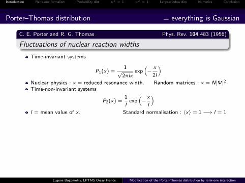
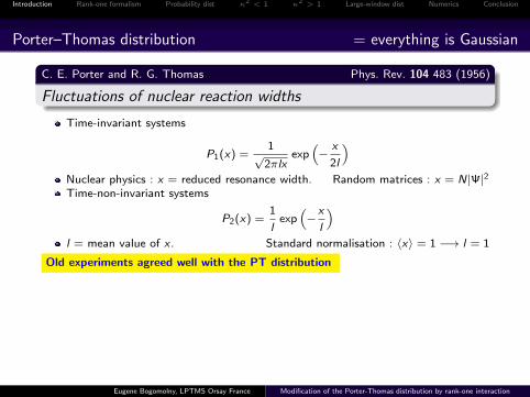
Porter–Thomas distribution = everything is Gaussian
C. E. Porter and R. G. Thomas Phys. Rev. 104 483 (1956)
Fluctuations of nuclear reaction widths
Time-invariant systems
P1(x) =1
√2πlx
exp(−
x
2l
)Nuclear physics : x = reduced resonance width. Random matrices : x = N|Ψ|2Time-non-invariant systems
P2(x) =1
lexp
(−x
l
)l = mean value of x . Standard normalisation : 〈x〉 = 1 −→ l = 1
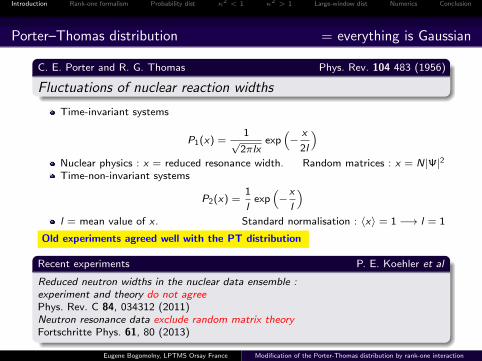
Old experiments agreed well with the PT distribution
Recent experiments P. E. Koehler et al
Reduced neutron widths in the nuclear data ensemble :experiment and theory do not agreePhys. Rev. C 84, 034312 (2011)Neutron resonance data exclude random matrix theoryFortschritte Phys. 61, 80 (2013)
Eugene Bogomolny, LPTMS Orsay France Modification of the Porter-Thomas distribution by rank-one interaction
Introduction Rank-one formalism Probability dist κ2 < 1 κ2 > 1 Large-window dist Numerics Conclusion
Porter–Thomas distribution = everything is Gaussian
C. E. Porter and R. G. Thomas Phys. Rev. 104 483 (1956)
Fluctuations of nuclear reaction widths
Time-invariant systems
P1(x) =1
√2πlx
exp(−
x
2l
)Nuclear physics : x = reduced resonance width. Random matrices : x = N|Ψ|2Time-non-invariant systems
P2(x) =1
lexp
(−x
l
)l = mean value of x . Standard normalisation : 〈x〉 = 1 −→ l = 1
Old experiments agreed well with the PT distribution
Recent experiments P. E. Koehler et al
Reduced neutron widths in the nuclear data ensemble :experiment and theory do not agreePhys. Rev. C 84, 034312 (2011)Neutron resonance data exclude random matrix theoryFortschritte Phys. 61, 80 (2013)
Eugene Bogomolny, LPTMS Orsay France Modification of the Porter-Thomas distribution by rank-one interaction
Introduction Rank-one formalism Probability dist κ2 < 1 κ2 > 1 Large-window dist Numerics Conclusion
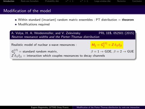
Modification of the model
Within standard (invariant) random matrix ensembles : PT distribution = theorem
Modifications required
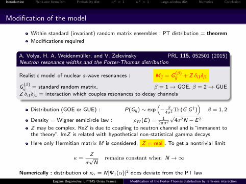
A. Volya, H. A. Weidenmuller, and V. Zelevinsky PRL 115, 052501 (2015)Neutron resonance widths and the Porter-Thomas distribution
Realistic model of nuclear s-wave resonances : Mij = G(β)ij + Z δi1δj1
G(β)ij = standard random matrix, β = 1→ GOE, β = 2→ GUE
Z δi1δj1 = interaction which couples resonances to decay channels
Distribution (GOE or GUE) : P(Gij ) ∼ exp(− β
4σ2 Tr (G G†))
β = 1, 2
Density = Wigner semicircle law : ρW (E) = 12πσ2
√4σ2N − E2
Z may be complex. ReZ is due to coupling to neutron channel and is ”immanent tothe theory”. ImZ is related with hypothetical non-statistical gamma decays
Here only Hermitian matrix M is considered, Z = real . To get a nontrivial limit
κ =Z
σ√N
remains constant when N →∞
Numerically : distribution of xα = N|Ψ1(α)|2 does deviate from the PT law
Eugene Bogomolny, LPTMS Orsay France Modification of the Porter-Thomas distribution by rank-one interaction
Introduction Rank-one formalism Probability dist κ2 < 1 κ2 > 1 Large-window dist Numerics Conclusion
Modification of the model
Within standard (invariant) random matrix ensembles : PT distribution = theorem
Modifications required
A. Volya, H. A. Weidenmuller, and V. Zelevinsky PRL 115, 052501 (2015)Neutron resonance widths and the Porter-Thomas distribution
Realistic model of nuclear s-wave resonances : Mij = G(β)ij + Z δi1δj1
G(β)ij = standard random matrix, β = 1→ GOE, β = 2→ GUE
Z δi1δj1 = interaction which couples resonances to decay channels
Distribution (GOE or GUE) : P(Gij ) ∼ exp(− β
4σ2 Tr (G G†))
β = 1, 2
Density = Wigner semicircle law : ρW (E) = 12πσ2
√4σ2N − E2
Z may be complex. ReZ is due to coupling to neutron channel and is ”immanent tothe theory”. ImZ is related with hypothetical non-statistical gamma decays
Here only Hermitian matrix M is considered, Z = real . To get a nontrivial limit
κ =Z
σ√N
remains constant when N →∞
Numerically : distribution of xα = N|Ψ1(α)|2 does deviate from the PT law
Eugene Bogomolny, LPTMS Orsay France Modification of the Porter-Thomas distribution by rank-one interaction
Introduction Rank-one formalism Probability dist κ2 < 1 κ2 > 1 Large-window dist Numerics Conclusion
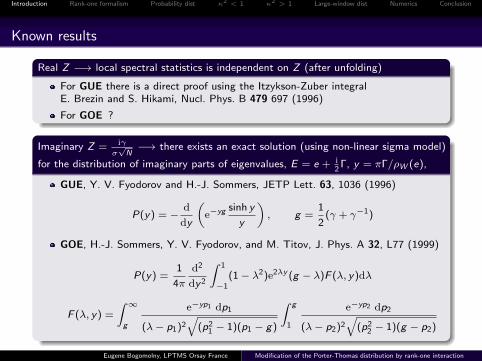
Known results
Real Z −→ local spectral statistics is independent on Z (after unfolding)
For GUE there is a direct proof using the Itzykson-Zuber integralE. Brezin and S. Hikami, Nucl. Phys. B 479 697 (1996)
For GOE ?
Imaginary Z = iγ
σ√N−→ there exists an exact solution (using non-linear sigma model)
for the distribution of imaginary parts of eigenvalues, E = e + i2
Γ, y = πΓ/ρW (e),
GUE, Y. V. Fyodorov and H.-J. Sommers, JETP Lett. 63, 1036 (1996)
P(y) = −d
dy
(e−yg sinh y
y
), g =
1
2(γ + γ−1)
GOE, H.-J. Sommers, Y. V. Fyodorov, and M. Titov, J. Phys. A 32, L77 (1999)
P(y) =1
4π
d2
dy2
∫ 1
−1(1− λ2)e2λy (g − λ)F (λ, y)dλ
F (λ, y) =
∫ ∞g
e−yp1 dp1
(λ− p1)2√
(p21 − 1)(p1 − g)
∫ g
1
e−yp2 dp2
(λ− p2)2√
(p22 − 1)(g − p2)
Eugene Bogomolny, LPTMS Orsay France Modification of the Porter-Thomas distribution by rank-one interaction
Introduction Rank-one formalism Probability dist κ2 < 1 κ2 > 1 Large-window dist Numerics Conclusion
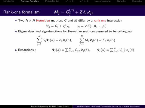
Rank-one formalism Mij = G(β)ij + Z δi1δj1
Two N × N Hermitian matrices G and M differ by a rank-one interaction
Mij = Gij + v∗i vj , vj =√Z(1, 0, . . . , 0)
Eigenvalues and eigenfunctions for Hermitian matrices assumed to be orthogonal
N∑j=1
GijΦj (α) = eαΦi (α),N∑j=1
MijΨj (α) = EαΨi (α)
Expansions : Ψj (α) =∑Nβ=1 CαβΦj (β), Φj (α) =
∑Nβ=1 C
−1αβΨj (β)
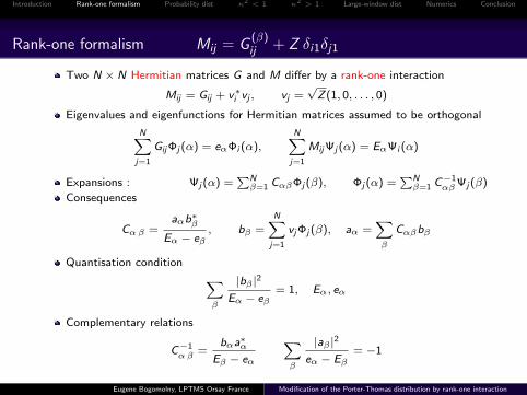
Consequences
Cαβ =aαb∗β
Eα − eβ, bβ =
N∑j=1
vjΦj (β), aα =∑β
Cαβbβ
Quantisation condition ∑β
|bβ |2
Eα − eβ= 1, Eα, eα
Complementary relations
C−1αβ =
bαa∗αEβ − eα
∑β
|aβ |2
eα − Eβ= −1
Eugene Bogomolny, LPTMS Orsay France Modification of the Porter-Thomas distribution by rank-one interaction
Introduction Rank-one formalism Probability dist κ2 < 1 κ2 > 1 Large-window dist Numerics Conclusion
Rank-one formalism Mij = G(β)ij + Z δi1δj1
Two N × N Hermitian matrices G and M differ by a rank-one interaction
Mij = Gij + v∗i vj , vj =√Z(1, 0, . . . , 0)
Eigenvalues and eigenfunctions for Hermitian matrices assumed to be orthogonal
N∑j=1
GijΦj (α) = eαΦi (α),N∑j=1
MijΨj (α) = EαΨi (α)
Expansions : Ψj (α) =∑Nβ=1 CαβΦj (β), Φj (α) =
∑Nβ=1 C
−1αβΨj (β)
Consequences
Cαβ =aαb∗β
Eα − eβ, bβ =
N∑j=1
vjΦj (β), aα =∑β
Cαβbβ
Quantisation condition ∑β
|bβ |2
Eα − eβ= 1, Eα, eα
Complementary relations
C−1αβ =
bαa∗αEβ − eα
∑β
|aβ |2
eα − Eβ= −1
Eugene Bogomolny, LPTMS Orsay France Modification of the Porter-Thomas distribution by rank-one interaction
Introduction Rank-one formalism Probability dist κ2 < 1 κ2 > 1 Large-window dist Numerics Conclusion
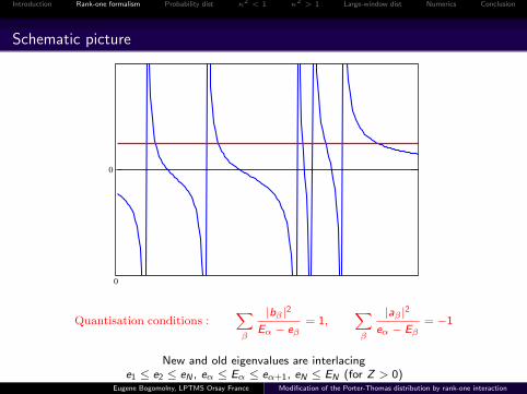
Schematic picture
0
0
Quantisation conditions :∑β
|bβ |2
Eα − eβ= 1,
∑β
|aβ |2
eα − Eβ= −1
New and old eigenvalues are interlacinge1 ≤ e2 ≤ eN , eα ≤ Eα ≤ eα+1, eN ≤ EN (for Z > 0)
Eugene Bogomolny, LPTMS Orsay France Modification of the Porter-Thomas distribution by rank-one interaction
Introduction Rank-one formalism Probability dist κ2 < 1 κ2 > 1 Large-window dist Numerics Conclusion
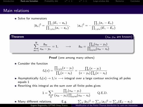
Main relations
Solve for numerators
|bα|2 =
∏γ(Eγ − eα)∏γ 6=α(eγ − eα)
, |aα|2 = −∏γ(eγ − Eα)∏
γ 6=α(Eγ − Eα)
Theorem (xm, ym are known)
N∑m=1
bm
xm − yn= 1, −→ bm =
∏n(xm − yn)∏
s 6=m(xm − xs)
Proof (one among many others)
Consider the function
fn(x) =
∏r 6=n(x − yr )∏s(x − xs)
=
∏r (x − yr )
(x − yn)∏
s(x − xs)
Asymptotically fn(x)→ 1/x −→ integral over a large contour encircling all polesequals 1Rewriting this integral as the sum over all finite poles gives
1 =∑m
∏r (xm − yr )
(xm − yn)∏
s 6=m(xm − xs)Q.E.D.
Many different relations. E.g.∑β |bβ |2 =
∑β |aβ |2 =
∑β(Eβ − eβ)
Eugene Bogomolny, LPTMS Orsay France Modification of the Porter-Thomas distribution by rank-one interaction
Introduction Rank-one formalism Probability dist κ2 < 1 κ2 > 1 Large-window dist Numerics Conclusion
Initial probability distribution
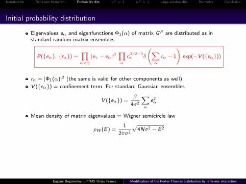
Eigenvalues eα and eigenfunctions Φ1(α) of matrix Gβ are distributed as instandard random matrix ensembles
P({eα}, {rα}) ∼∏α<γ
|eγ − eα|β∏α
rβ/2−1α δ
(∑α
rα − 1
)exp(−V ({eα}))
rα = |Φ1(α)|2 (the same is valid for other components as well)
V ({eα}) = confinement term. For standard Gaussian ensembles
V ({eα}) =β
4σ2
∑α
e2α
Mean density of matrix eigenvalues = Wigner semicircle law
ρW (E) =1
2πσ2
√4Nσ2 − E2
Main question
How new eigenvectors Ψ1(α) and new eigenvalues Eα are distributed ?
Two steps of changing variables : (eα,Φ1(α)) −→ (eα,Eα) −→ (Ψ1(α),Eα)
Eugene Bogomolny, LPTMS Orsay France Modification of the Porter-Thomas distribution by rank-one interaction
Introduction Rank-one formalism Probability dist κ2 < 1 κ2 > 1 Large-window dist Numerics Conclusion
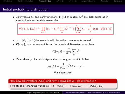
Initial probability distribution
Eigenvalues eα and eigenfunctions Φ1(α) of matrix Gβ are distributed as instandard random matrix ensembles
P({eα}, {rα}) ∼∏α<γ
|eγ − eα|β∏α
rβ/2−1α δ
(∑α
rα − 1
)exp(−V ({eα}))
rα = |Φ1(α)|2 (the same is valid for other components as well)
V ({eα}) = confinement term. For standard Gaussian ensembles
V ({eα}) =β
4σ2
∑α
e2α
Mean density of matrix eigenvalues = Wigner semicircle law
ρW (E) =1
2πσ2
√4Nσ2 − E2
Main question
How new eigenvectors Ψ1(α) and new eigenvalues Eα are distributed ?
Two steps of changing variables : (eα,Φ1(α)) −→ (eα,Eα) −→ (Ψ1(α),Eα)
Eugene Bogomolny, LPTMS Orsay France Modification of the Porter-Thomas distribution by rank-one interaction
Introduction Rank-one formalism Probability dist κ2 < 1 κ2 > 1 Large-window dist Numerics Conclusion
Joint distribution of old and new eigenvalues
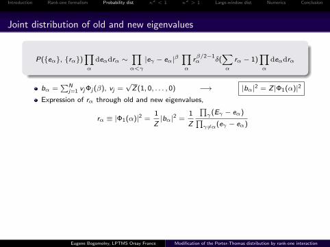
P({eα}, {rα})∏α
deαdrα ∼∏α<γ
|eγ − eα|β∏α
rβ/2−1α δ(
∑α
rα − 1)∏α
deαdrα
bα =∑N
j=1 vjΦj (β), vj =√Z(1, 0, . . . , 0) −→ |bα|2 = Z |Φ1(α)|2
Expression of rα through old and new eigenvalues,
rα ≡ |Φ1(α)|2 =1
Z|bα|2 =
1
Z
∏γ(Eγ − eα)∏γ 6=α(eγ − eα)
Change of variables : N quantities rα −→ N quantities Eα
Derivatives : ∂rα/∂Eγ = rα/(Eγ − eα)
Cauchy determinant : det( 1xm−yn
) =∏
i<j (xi−xj )∏
i<j (yj−yi )∏i,j (xi−yj )
Jacobian
det
(∂rα
∂Eγ
)= (
∏α
rα) det
(1
Eγ − eα
)= (∏α
rα)
∏α<β(Eα − Eβ)(eβ − eα)∏
α,β(Eα − eβ)
=1
ZN
∏α<γ
(Eγ − Eα)
(eα − eγ),
∑α
rα =1
Z
∑α
(Eα − eα)
Eugene Bogomolny, LPTMS Orsay France Modification of the Porter-Thomas distribution by rank-one interaction
Introduction Rank-one formalism Probability dist κ2 < 1 κ2 > 1 Large-window dist Numerics Conclusion
Joint distribution of old and new eigenvalues
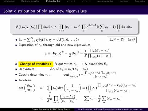
P({eα}, {rα})∏α
deαdrα ∼∏α<γ
|eγ − eα|β∏α
rβ/2−1α δ(
∑α
rα − 1)∏α
deαdrα
bα =∑N
j=1 vjΦj (β), vj =√Z(1, 0, . . . , 0) −→ |bα|2 = Z |Φ1(α)|2
Expression of rα through old and new eigenvalues,
rα ≡ |Φ1(α)|2 =1
Z|bα|2 =
1
Z
∏γ(Eγ − eα)∏γ 6=α(eγ − eα)
Change of variables : N quantities rα −→ N quantities Eα
Derivatives : ∂rα/∂Eγ = rα/(Eγ − eα)
Cauchy determinant : det( 1xm−yn
) =∏
i<j (xi−xj )∏
i<j (yj−yi )∏i,j (xi−yj )
Jacobian
det
(∂rα
∂Eγ
)= (
∏α
rα) det
(1
Eγ − eα
)= (∏α
rα)
∏α<β(Eα − Eβ)(eβ − eα)∏
α,β(Eα − eβ)
=1
ZN
∏α<γ
(Eγ − Eα)
(eα − eγ),
∑α
rα =1
Z
∑α
(Eα − eα)
Eugene Bogomolny, LPTMS Orsay France Modification of the Porter-Thomas distribution by rank-one interaction
Introduction Rank-one formalism Probability dist κ2 < 1 κ2 > 1 Large-window dist Numerics Conclusion
Change from old eigenvalues to new eigenfunctions
I. L. Aleiner and K. A. Matveev Shifts of random energy levels by a local perturbation,PRL 80, 814 (1998)
P({eα}, {Eα}) ∼∏γ>α(eγ − eα)(Eγ − Eα)∏γ,α |eγ − Eα|β/2−1
δ
(∑α
(Eα − eα)− Z
)∏α
deαdEα
Ψ1(α) =∑β CαβΦ1(β) = 1√
Z
∑β Cαβbβ = aα√
Z
∑β|bβ |2
Eα−eβ= aα√
Z
Expression of rα through old and new eigenvalues
zα = |Ψ1(α)|2 =1
Z|aα|2 =
1
Z
∏γ(Eα − eγ)∏
γ 6=α(Eα − Eγ)
N quantities rα −→ N quantities eα. Derivatives : ∂zα∂eγ
= − zαEα−eγ
Jacobian
det
(∂zα
∂eβ
)=
1
ZN
∏α<γ
(eγ − eα)
(Eα − Eγ)
Identities∏α,γ
(Eα − eγ) =∏α
zα( ∏α<γ
(Eα − Eγ))2,
∑α
zα =1
Z
∑α
(Eα − eα)
Eugene Bogomolny, LPTMS Orsay France Modification of the Porter-Thomas distribution by rank-one interaction
Introduction Rank-one formalism Probability dist κ2 < 1 κ2 > 1 Large-window dist Numerics Conclusion
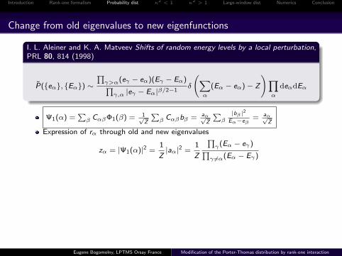
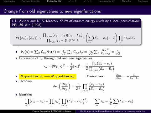
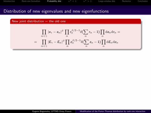
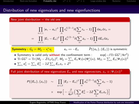
Distribution of new eigenvalues and new eigenfunctions
New joint distribution = the old one
∏α<γ
|eγ − eα|β∏α
rβ/2−1α δ(
∑α
rα − 1)∏α
deαdrα =
=∏α<γ
|Eγ − Eα|β∏α
zβ/2−1α δ(
∑α
zα − 1)∏α
dEαdzα
Symmetry : Gij = Mij − v∗i vj eα ↔ −Eα P({eα}, {Eα}) is symmetric
Symmetry is valid only without the confinement term : exp(−βTrGG†/4σ2)
TrGG† = Tr (Mij − Zδi1δj1)2, Mij =∑α EαΨi (α)Ψ∗j (α), M11 =
∑α Eα|Ψ1(α)|2∑
α e2α =
∑α E2
α − 2Z∑α Eαzα + Z2
Full joint distribution of new eigenvalues Eα and new eigenvectors, zα ≡ |Ψ1(α)|2
P({Eα}, {zα}) ∼∏α<β
|Eβ − Eα|β∏α
zβ/2−1α δ(
∑α
zα − 1)
× exp[−
β
4σ2
(∑α
E2α − 2Z
∑α
Eαzα)]
Eugene Bogomolny, LPTMS Orsay France Modification of the Porter-Thomas distribution by rank-one interaction
Introduction Rank-one formalism Probability dist κ2 < 1 κ2 > 1 Large-window dist Numerics Conclusion
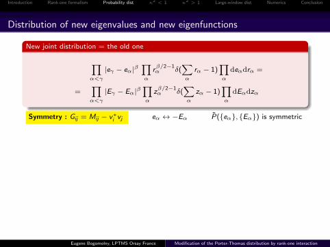
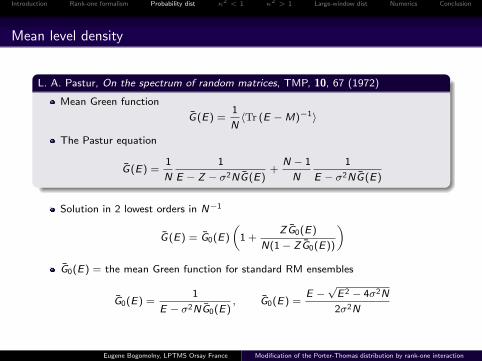
Mean level density
L. A. Pastur, On the spectrum of random matrices, TMP, 10, 67 (1972)
Mean Green function
G(E) =1
N〈Tr (E −M)−1〉
The Pastur equation
G(E) =1
N
1
E − Z − σ2NG(E)+
N − 1
N
1
E − σ2NG(E)
Solution in 2 lowest orders in N−1
G(E) = G0(E)
(1 +
ZG0(E)
N(1− ZG0(E))
)G0(E) = the mean Green function for standard RM ensembles
G0(E) =1
E − σ2NG0(E), G0(E) =
E −√E2 − 4σ2N
2σ2N
Eugene Bogomolny, LPTMS Orsay France Modification of the Porter-Thomas distribution by rank-one interaction
Introduction Rank-one formalism Probability dist κ2 < 1 κ2 > 1 Large-window dist Numerics Conclusion
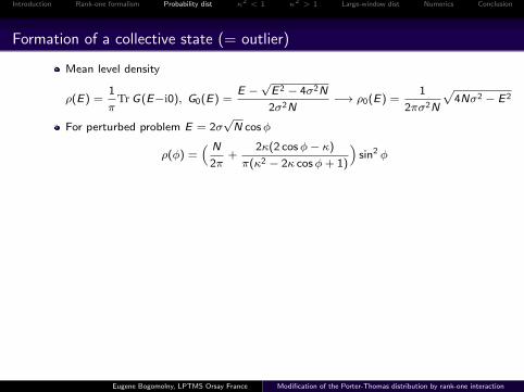
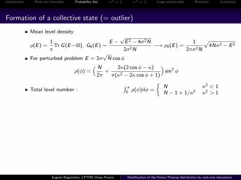
Formation of a collective state (= outlier)
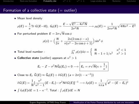
Mean level density
ρ(E) =1
πTrG(E−i0), G0(E) =
E −√E2 − 4σ2N
2σ2N−→ ρ0(E) =
1
2πσ2N
√4Nσ2 − E2
For perturbed problem E = 2σ√N cosφ
ρ(φ) =( N
2π+
2κ(2 cosφ− κ)
π(κ2 − 2κ cosφ+ 1)
)sin2 φ
Total level number :∫ π
0 ρ(φ)dφ =
{N κ2 < 1N − 1 + 1/κ2 κ2 > 1
Collective state (outlier) appears at κ2 > 1
Ec − Z − σ2NG0(Ec) = 0 −→ Ec = σ√N(κ+
1
κ)
Close to Ec G(E) ≈ G0(E) + δG(E) (a = 2σ(1− κ−2))
δG(E) =1
N[κ2
κ2 − 1(E−Ec)−σ2NδG(E)]−1 −→ δρ(E) =
1
πσa
√a2 − (E − Ec)2
∫δρ(E)dE = 1− κ−2. Total :
∫ρ(E)dE = N
Exact result : E − Ec = Gaussian variable with mean= 0, variance= 2(κ2−1)σ2
βκ2
Eugene Bogomolny, LPTMS Orsay France Modification of the Porter-Thomas distribution by rank-one interaction
Introduction Rank-one formalism Probability dist κ2 < 1 κ2 > 1 Large-window dist Numerics Conclusion
Formation of a collective state (= outlier)
Mean level density
ρ(E) =1
πTrG(E−i0), G0(E) =
E −√E2 − 4σ2N
2σ2N−→ ρ0(E) =
1
2πσ2N
√4Nσ2 − E2
For perturbed problem E = 2σ√N cosφ
ρ(φ) =( N
2π+
2κ(2 cosφ− κ)
π(κ2 − 2κ cosφ+ 1)
)sin2 φ
Total level number :∫ π
0 ρ(φ)dφ =
{N κ2 < 1N − 1 + 1/κ2 κ2 > 1
Collective state (outlier) appears at κ2 > 1
Ec − Z − σ2NG0(Ec) = 0 −→ Ec = σ√N(κ+
1
κ)
Close to Ec G(E) ≈ G0(E) + δG(E) (a = 2σ(1− κ−2))
δG(E) =1
N[κ2
κ2 − 1(E−Ec)−σ2NδG(E)]−1 −→ δρ(E) =
1
πσa
√a2 − (E − Ec)2
∫δρ(E)dE = 1− κ−2. Total :
∫ρ(E)dE = N
Exact result : E − Ec = Gaussian variable with mean= 0, variance= 2(κ2−1)σ2
βκ2
Eugene Bogomolny, LPTMS Orsay France Modification of the Porter-Thomas distribution by rank-one interaction
Introduction Rank-one formalism Probability dist κ2 < 1 κ2 > 1 Large-window dist Numerics Conclusion
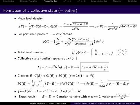
Case κ2 < 1
zα = |Ψ1(α)|2 for all energies Eα are O(N−1)Condition
∑α zα = 1 can be taken into account by the Lagrange multiplier
δ(∑α
zα − 1) −→ exp(−µ(∑α
zα − 1))
zα = independent, each zα ≡ z(Eα) has PDF
P(z,E) =(µ−
Z
2σ2E)β/2
(πz)β/2−1 exp
(−(µ−
βZ
2σ2E)z
)µ has to be calculated from normalisation :
∑α zα = 1∑
α
∫ ∞0
z P(z,Eα) dz = 1,∑α
1
E − Eα=
Z
σ2, E =
2µσ2
βZ
The sum is mean unperturbed Green function, G0(E)
G0(E) =1
N〈Tr (E − G)−1〉 =
E −√E2 − 4σ2N
2σ2N−→ µ = βN
κ2 + 1
2
Distribution of perturbed problem = local PT distribution
Pβ(x) =1
(2πx)1−β/2(l(E))β/2exp
(−
βx
2l(E)
), l(E) =
(κ2 + 1−
κ
σ√NE
)−1
Eugene Bogomolny, LPTMS Orsay France Modification of the Porter-Thomas distribution by rank-one interaction
Introduction Rank-one formalism Probability dist κ2 < 1 κ2 > 1 Large-window dist Numerics Conclusion
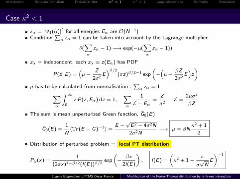
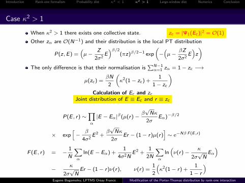
Case κ2 > 1
When κ2 > 1 there exists one collective state. zc = |Ψ1(Ec)|2 = O(1)
Other zα are O(N−1) and their distribution is the local PT distribution
P(z,E) =(µ−
Z
2σ2E)β/2
(πz)β/2−1 exp
(−(µ−
βZ
2σ2E)z
)The only difference is that their normalisation is
∑N−1α=1 zα = 1− zc −→
µ(zc) =βN
2
(κ2(1− zc) +
1
1− zc
)
Calculation of Ec and zcJoint distribution of E ≡ Ec and r ≡ zc
P(E , r) ∼∏α
|E − Eα|β(µ(r)−β√Nκ
2σEα)−β/2
× exp[−
β
4σ2E2 +
β√Nκ
2σEr − (1− r)µ(r)
]∼ e−Nβ F (E ,r)
F (E , r) = −1
N
∑α
ln(E − Eα) +1
4σ2NE2 +
1
2N
∑α
ln(ν(r)−
κ
2σ√NEα)
−κ
2σ√NEr − (1− r)ν(r), ν(r) =
1
2
(κ2(1− r) +
1
1− r
)
Eugene Bogomolny, LPTMS Orsay France Modification of the Porter-Thomas distribution by rank-one interaction
Introduction Rank-one formalism Probability dist κ2 < 1 κ2 > 1 Large-window dist Numerics Conclusion
Case κ2 > 1
When κ2 > 1 there exists one collective state. zc = |Ψ1(Ec)|2 = O(1)
Other zα are O(N−1) and their distribution is the local PT distribution
P(z,E) =(µ−
Z
2σ2E)β/2
(πz)β/2−1 exp
(−(µ−
βZ
2σ2E)z
)The only difference is that their normalisation is
∑N−1α=1 zα = 1− zc −→
µ(zc) =βN
2
(κ2(1− zc) +
1
1− zc
)Calculation of Ec and zc
Joint distribution of E ≡ Ec and r ≡ zc
P(E , r) ∼∏α
|E − Eα|β(µ(r)−β√Nκ
2σEα)−β/2
× exp[−
β
4σ2E2 +
β√Nκ
2σEr − (1− r)µ(r)
]∼ e−Nβ F (E ,r)
F (E , r) = −1
N
∑α
ln(E − Eα) +1
4σ2NE2 +
1
2N
∑α
ln(ν(r)−
κ
2σ√NEα)
−κ
2σ√NEr − (1− r)ν(r), ν(r) =
1
2
(κ2(1− r) +
1
1− r
)Eugene Bogomolny, LPTMS Orsay France Modification of the Porter-Thomas distribution by rank-one interaction
Introduction Rank-one formalism Probability dist κ2 < 1 κ2 > 1 Large-window dist Numerics Conclusion
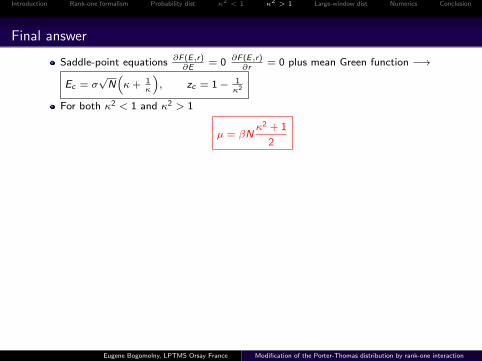
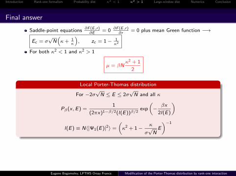
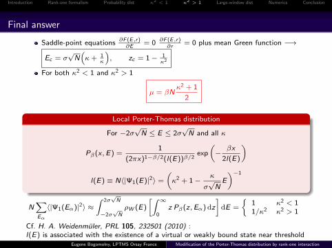
Final answer
Saddle-point equations ∂F (E ,r)∂E
= 0 ∂F (E ,r)∂r
= 0 plus mean Green function −→
Ec = σ√N(κ+ 1
κ
), zc = 1− 1
κ2
For both κ2 < 1 and κ2 > 1
µ = βNκ2 + 1
2
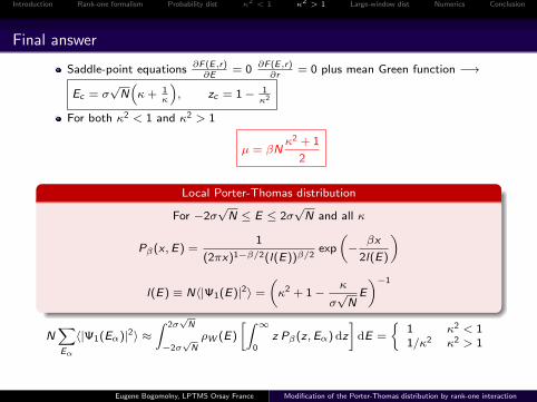
Local Porter-Thomas distribution
For −2σ√N ≤ E ≤ 2σ
√N and all κ
Pβ(x ,E) =1
(2πx)1−β/2(l(E))β/2exp
(−
βx
2l(E)
)
l(E) ≡ N〈|Ψ1(E)|2〉 =
(κ2 + 1−
κ
σ√NE
)−1
N∑Eα
〈|Ψ1(Eα)|2〉 ≈∫ 2σ
√N
−2σ√NρW (E)
[∫ ∞0
z Pβ(z,Eα) dz
]dE =
{1 κ2 < 11/κ2 κ2 > 1
Cf. H. A. Weidenmuler, PRL 105, 232501 (2010) :l(E) is associated with the existence of a virtual or weakly bound state near threshold
Eugene Bogomolny, LPTMS Orsay France Modification of the Porter-Thomas distribution by rank-one interaction
Introduction Rank-one formalism Probability dist κ2 < 1 κ2 > 1 Large-window dist Numerics Conclusion
Final answer
Saddle-point equations ∂F (E ,r)∂E
= 0 ∂F (E ,r)∂r
= 0 plus mean Green function −→
Ec = σ√N(κ+ 1
κ
), zc = 1− 1
κ2
For both κ2 < 1 and κ2 > 1
µ = βNκ2 + 1
2
Local Porter-Thomas distribution
For −2σ√N ≤ E ≤ 2σ
√N and all κ
Pβ(x ,E) =1
(2πx)1−β/2(l(E))β/2exp
(−
βx
2l(E)
)
l(E) ≡ N〈|Ψ1(E)|2〉 =
(κ2 + 1−
κ
σ√NE
)−1
N∑Eα
〈|Ψ1(Eα)|2〉 ≈∫ 2σ
√N
−2σ√NρW (E)
[∫ ∞0
z Pβ(z,Eα) dz
]dE =
{1 κ2 < 11/κ2 κ2 > 1
Cf. H. A. Weidenmuler, PRL 105, 232501 (2010) :l(E) is associated with the existence of a virtual or weakly bound state near threshold
Eugene Bogomolny, LPTMS Orsay France Modification of the Porter-Thomas distribution by rank-one interaction
Introduction Rank-one formalism Probability dist κ2 < 1 κ2 > 1 Large-window dist Numerics Conclusion
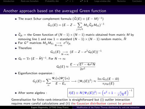
Another approach based on the averaged Green function
The exact Schur complement formula (G(E) ≡ (E −M)−1)
G11(E) = (E − Z −∑j,k 6=1
M1j GjkMk1)−1
Gjk = the Green function of (N − 1)× (N − 1) matrix obtained from matrix M by
removing line 1 and row 1 = standard (N − 1)× (N − 1) random matrix, HFor Gβ matrices M1jMk1 −→
N→∞σ2δjk
ThereforeG11(E) −→
N→∞(E − Z − σ2G0(E))−1
G0 = Tr (E − H)−1. For N →∞
G0(E) ≈E −√E2 − 4σ2N
2σ2
Eigenfunction expansion :
Gij (E) =∑α
Ψi (α)Ψ∗j (α)
E − Eα−→ 〈|Ψ1(E)|2〉 ≈
ImG11(E − i0)
πρW (E)
After some algebra : l(E) ≡ N〈|Ψ1(E)|2〉 =(κ2 + 1− κ
σ√NE)−1
Generalisation for finite rank-interaction is straightforward but (i) outlier interactionrequires more careful calculations and (ii) the Gaussian distribution cannot be proved
Eugene Bogomolny, LPTMS Orsay France Modification of the Porter-Thomas distribution by rank-one interaction
Introduction Rank-one formalism Probability dist κ2 < 1 κ2 > 1 Large-window dist Numerics Conclusion
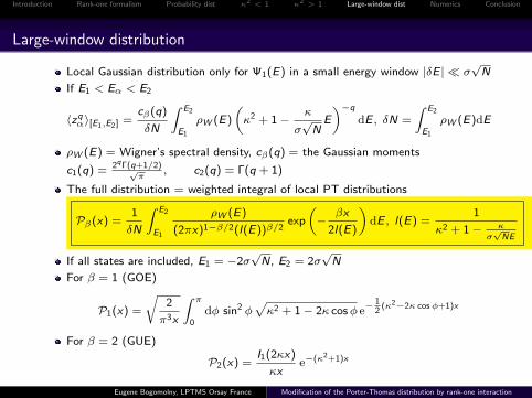
Large-window distribution
Local Gaussian distribution only for Ψ1(E) in a small energy window |δE | � σ√N
If E1 < Eα < E2
〈zqα〉[E1,E2] =cβ(q)
δN
∫ E2
E1
ρW (E)
(κ2 + 1−
κ
σ√NE
)−q
dE , δN =
∫ E2
E1
ρW (E)dE
ρW (E) = Wigner’s spectral density, cβ(q) = the Gaussian moments
c1(q) = 2qΓ(q+1/2)√π
, c2(q) = Γ(q + 1)
The full distribution = weighted integral of local PT distributions
Pβ(x) =1
δN
∫ E2
E1
ρW (E)
(2πx)1−β/2(l(E))β/2exp
(−
βx
2l(E)
)dE , l(E) =
1
κ2 + 1− κ
σ√
NE
If all states are included, E1 = −2σ√N, E2 = 2σ
√N
For β = 1 (GOE)
P1(x) =
√2
π3x
∫ π
0dφ sin2 φ
√κ2 + 1− 2κ cosφ e−
12
(κ2−2κ cosφ+1)x
For β = 2 (GUE)
P2(x) =I1(2κx)
κxe−(κ2+1)x
Eugene Bogomolny, LPTMS Orsay France Modification of the Porter-Thomas distribution by rank-one interaction
Introduction Rank-one formalism Probability dist κ2 < 1 κ2 > 1 Large-window dist Numerics Conclusion
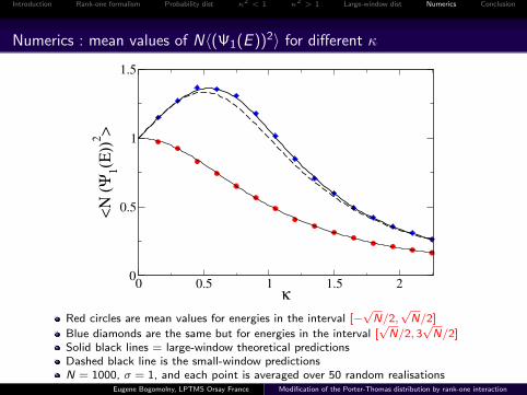
Numerics : mean values of N〈(Ψ1(E ))2〉 for different κ
0 0.5 1 1.5 2
κ
0
0.5
1
1.5
<Ν
(Ψ
1(Ε
))2>
Red circles are mean values for energies in the interval [−√N/2,
√N/2]
Blue diamonds are the same but for energies in the interval [√N/2, 3
√N/2]
Solid black lines = large-window theoretical predictionsDashed black line is the small-window predictionsN = 1000, σ = 1, and each point is averaged over 50 random realisations
Eugene Bogomolny, LPTMS Orsay France Modification of the Porter-Thomas distribution by rank-one interaction
Introduction Rank-one formalism Probability dist κ2 < 1 κ2 > 1 Large-window dist Numerics Conclusion
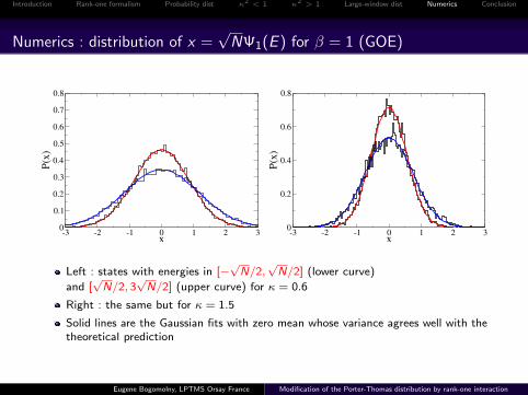
Numerics : distribution of x =√
NΨ1(E ) for β = 1 (GOE)
-3 -2 -1 0 1 2 3x
0
0.1
0.2
0.3
0.4
0.5
0.6
0.7
0.8
P(x
)
-3 -2 -1 0 1 2 3x
0
0.2
0.4
0.6
0.8
P(x
)Left : states with energies in [−
√N/2,
√N/2] (lower curve)
and [√N/2, 3
√N/2] (upper curve) for κ = 0.6
Right : the same but for κ = 1.5
Solid lines are the Gaussian fits with zero mean whose variance agrees well with thetheoretical prediction
Eugene Bogomolny, LPTMS Orsay France Modification of the Porter-Thomas distribution by rank-one interaction
Introduction Rank-one formalism Probability dist κ2 < 1 κ2 > 1 Large-window dist Numerics Conclusion
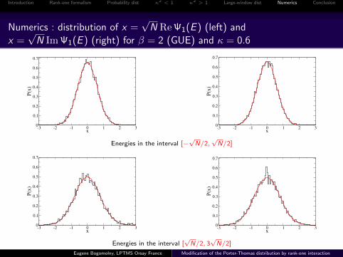
Numerics : distribution of x =√
N ReΨ1(E ) (left) and
x =√
N ImΨ1(E ) (right) for β = 2 (GUE) and κ = 0.6
-3 -2 -1 0 1 2 3x
0
0.1
0.2
0.3
0.4
0.5
0.6
0.7
P(x
)
-3 -2 -1 0 1 2 3x
0
0.1
0.2
0.3
0.4
0.5
0.6
0.7
P(x
)
Energies in the interval [−√N/2,
√N/2]
-3 -2 -1 0 1 2 3x
0
0.1
0.2
0.3
0.4
0.5
0.6
0.7
P(x
)
-3 -2 -1 0 1 2 3x
0
0.1
0.2
0.3
0.4
0.5
0.6
0.7
P(x
)
Energies in the interval [√N/2, 3
√N/2]
Eugene Bogomolny, LPTMS Orsay France Modification of the Porter-Thomas distribution by rank-one interaction
Introduction Rank-one formalism Probability dist κ2 < 1 κ2 > 1 Large-window dist Numerics Conclusion
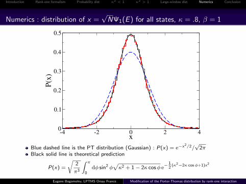
Numerics : distribution of x =√
NΨ1(E ) for all states, κ = .8, β = 1
-4 -2 0 2 4x
0
0.1
0.2
0.3
0.4
0.5
P(x
)
Blue dashed line is the PT distribution (Gaussian) : P(x) = e−x2/2/√
2πBlack solid line is theoretical prediction
P(x) =
√2
π3
∫ π
0dφ sin2 φ
√κ2 + 1− 2κ cosφ e−
12
(κ2−2κ cosφ+1)x2
Eugene Bogomolny, LPTMS Orsay France Modification of the Porter-Thomas distribution by rank-one interaction
Introduction Rank-one formalism Probability dist κ2 < 1 κ2 > 1 Large-window dist Numerics Conclusion
Conclusion
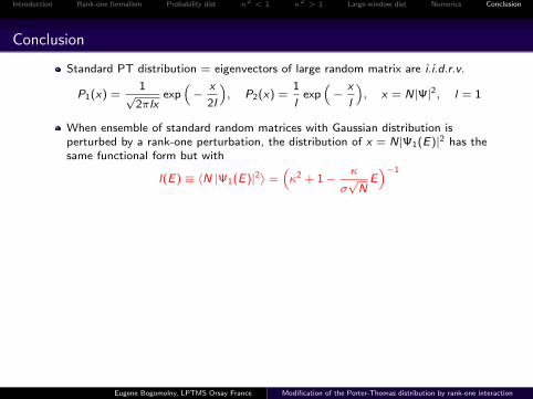
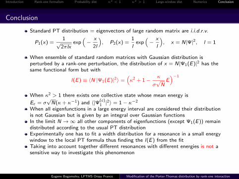
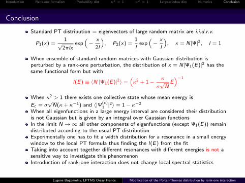
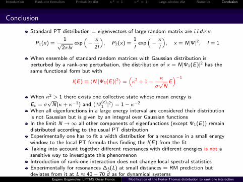
Standard PT distribution = eigenvectors of large random matrix are i.i.d.r.v.
P1(x) =1
√2πlx
exp(−
x
2l
), P2(x) =
1
lexp
(−
x
l
), x = N|Ψ|2, l = 1
When ensemble of standard random matrices with Gaussian distribution isperturbed by a rank-one perturbation, the distribution of x = N|Ψ1(E)|2 has thesame functional form but with
l(E) ≡ 〈N |Ψ1(E)|2〉 =(κ2 + 1−
κ
σ√NE)−1
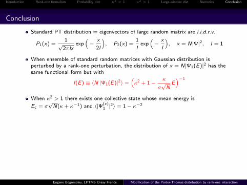
When κ2 > 1 there exists one collective state whose mean energy is
Ec = σ√N(κ+ κ−1) and 〈|Ψ(c)
1 |2〉 = 1− κ−2
When all eigenfunctions in a large energy interval are considered their distributionis not Gaussian but is given by an integral over Gaussian functionsIn the limit N →∞ all other components of eigenfunctions (except Ψ1(E)) remaindistributed according to the usual PT distributionExperimentally one has to fit a width distribution for a resonance in a small energywindow to the local PT formula thus finding the l(E) from the fitTaking into account together different resonances with different energies is not asensitive way to investigate this phenomenonIntroduction of rank-one interaction does not change local spectral statisticsExperimentally for resonances ∆3(L) at small distances = RM prediction butdeviates from it at L ≈ 40− 70 d as for dynamical systems
Eugene Bogomolny, LPTMS Orsay France Modification of the Porter-Thomas distribution by rank-one interaction
Introduction Rank-one formalism Probability dist κ2 < 1 κ2 > 1 Large-window dist Numerics Conclusion
Conclusion
Standard PT distribution = eigenvectors of large random matrix are i.i.d.r.v.
P1(x) =1
√2πlx
exp(−
x
2l
), P2(x) =
1
lexp
(−
x
l
), x = N|Ψ|2, l = 1
When ensemble of standard random matrices with Gaussian distribution isperturbed by a rank-one perturbation, the distribution of x = N|Ψ1(E)|2 has thesame functional form but with
l(E) ≡ 〈N |Ψ1(E)|2〉 =(κ2 + 1−
κ
σ√NE)−1
When κ2 > 1 there exists one collective state whose mean energy is
Ec = σ√N(κ+ κ−1) and 〈|Ψ(c)
1 |2〉 = 1− κ−2
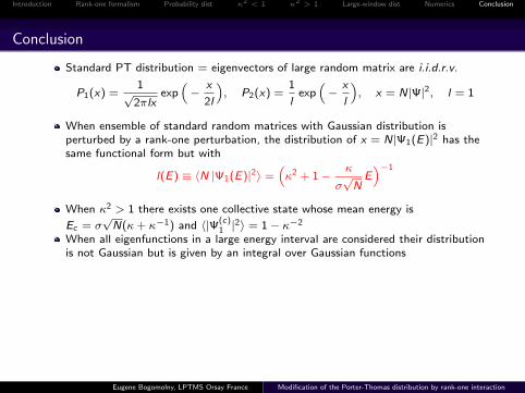
When all eigenfunctions in a large energy interval are considered their distributionis not Gaussian but is given by an integral over Gaussian functions
In the limit N →∞ all other components of eigenfunctions (except Ψ1(E)) remaindistributed according to the usual PT distributionExperimentally one has to fit a width distribution for a resonance in a small energywindow to the local PT formula thus finding the l(E) from the fitTaking into account together different resonances with different energies is not asensitive way to investigate this phenomenonIntroduction of rank-one interaction does not change local spectral statisticsExperimentally for resonances ∆3(L) at small distances = RM prediction butdeviates from it at L ≈ 40− 70 d as for dynamical systems
Eugene Bogomolny, LPTMS Orsay France Modification of the Porter-Thomas distribution by rank-one interaction
Introduction Rank-one formalism Probability dist κ2 < 1 κ2 > 1 Large-window dist Numerics Conclusion
Conclusion
Standard PT distribution = eigenvectors of large random matrix are i.i.d.r.v.
P1(x) =1
√2πlx
exp(−
x
2l
), P2(x) =
1
lexp
(−
x
l
), x = N|Ψ|2, l = 1
When ensemble of standard random matrices with Gaussian distribution isperturbed by a rank-one perturbation, the distribution of x = N|Ψ1(E)|2 has thesame functional form but with
l(E) ≡ 〈N |Ψ1(E)|2〉 =(κ2 + 1−
κ
σ√NE)−1
When κ2 > 1 there exists one collective state whose mean energy is
Ec = σ√N(κ+ κ−1) and 〈|Ψ(c)
1 |2〉 = 1− κ−2
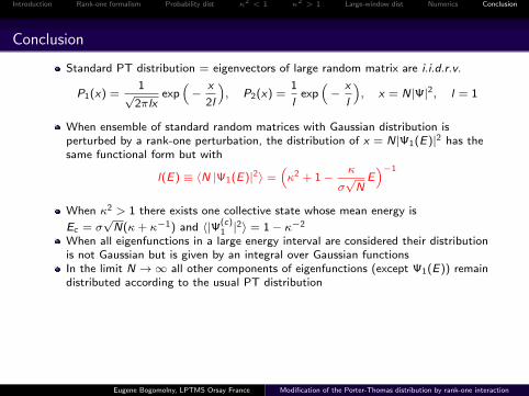
When all eigenfunctions in a large energy interval are considered their distributionis not Gaussian but is given by an integral over Gaussian functionsIn the limit N →∞ all other components of eigenfunctions (except Ψ1(E)) remaindistributed according to the usual PT distribution
Experimentally one has to fit a width distribution for a resonance in a small energywindow to the local PT formula thus finding the l(E) from the fitTaking into account together different resonances with different energies is not asensitive way to investigate this phenomenonIntroduction of rank-one interaction does not change local spectral statisticsExperimentally for resonances ∆3(L) at small distances = RM prediction butdeviates from it at L ≈ 40− 70 d as for dynamical systems
Eugene Bogomolny, LPTMS Orsay France Modification of the Porter-Thomas distribution by rank-one interaction
Introduction Rank-one formalism Probability dist κ2 < 1 κ2 > 1 Large-window dist Numerics Conclusion
Conclusion
Standard PT distribution = eigenvectors of large random matrix are i.i.d.r.v.
P1(x) =1
√2πlx
exp(−
x
2l
), P2(x) =
1
lexp
(−
x
l
), x = N|Ψ|2, l = 1
When ensemble of standard random matrices with Gaussian distribution isperturbed by a rank-one perturbation, the distribution of x = N|Ψ1(E)|2 has thesame functional form but with
l(E) ≡ 〈N |Ψ1(E)|2〉 =(κ2 + 1−
κ
σ√NE)−1
When κ2 > 1 there exists one collective state whose mean energy is
Ec = σ√N(κ+ κ−1) and 〈|Ψ(c)
1 |2〉 = 1− κ−2
When all eigenfunctions in a large energy interval are considered their distributionis not Gaussian but is given by an integral over Gaussian functionsIn the limit N →∞ all other components of eigenfunctions (except Ψ1(E)) remaindistributed according to the usual PT distributionExperimentally one has to fit a width distribution for a resonance in a small energywindow to the local PT formula thus finding the l(E) from the fitTaking into account together different resonances with different energies is not asensitive way to investigate this phenomenon
Introduction of rank-one interaction does not change local spectral statisticsExperimentally for resonances ∆3(L) at small distances = RM prediction butdeviates from it at L ≈ 40− 70 d as for dynamical systems
Eugene Bogomolny, LPTMS Orsay France Modification of the Porter-Thomas distribution by rank-one interaction
Introduction Rank-one formalism Probability dist κ2 < 1 κ2 > 1 Large-window dist Numerics Conclusion
Conclusion
Standard PT distribution = eigenvectors of large random matrix are i.i.d.r.v.
P1(x) =1
√2πlx
exp(−
x
2l
), P2(x) =
1
lexp
(−
x
l
), x = N|Ψ|2, l = 1
When ensemble of standard random matrices with Gaussian distribution isperturbed by a rank-one perturbation, the distribution of x = N|Ψ1(E)|2 has thesame functional form but with
l(E) ≡ 〈N |Ψ1(E)|2〉 =(κ2 + 1−
κ
σ√NE)−1
When κ2 > 1 there exists one collective state whose mean energy is
Ec = σ√N(κ+ κ−1) and 〈|Ψ(c)
1 |2〉 = 1− κ−2
When all eigenfunctions in a large energy interval are considered their distributionis not Gaussian but is given by an integral over Gaussian functionsIn the limit N →∞ all other components of eigenfunctions (except Ψ1(E)) remaindistributed according to the usual PT distributionExperimentally one has to fit a width distribution for a resonance in a small energywindow to the local PT formula thus finding the l(E) from the fitTaking into account together different resonances with different energies is not asensitive way to investigate this phenomenonIntroduction of rank-one interaction does not change local spectral statistics
Experimentally for resonances ∆3(L) at small distances = RM prediction butdeviates from it at L ≈ 40− 70 d as for dynamical systems
Eugene Bogomolny, LPTMS Orsay France Modification of the Porter-Thomas distribution by rank-one interaction
Introduction Rank-one formalism Probability dist κ2 < 1 κ2 > 1 Large-window dist Numerics Conclusion
Conclusion
Standard PT distribution = eigenvectors of large random matrix are i.i.d.r.v.
P1(x) =1
√2πlx
exp(−
x
2l
), P2(x) =
1
lexp
(−
x
l
), x = N|Ψ|2, l = 1
When ensemble of standard random matrices with Gaussian distribution isperturbed by a rank-one perturbation, the distribution of x = N|Ψ1(E)|2 has thesame functional form but with
l(E) ≡ 〈N |Ψ1(E)|2〉 =(κ2 + 1−
κ
σ√NE)−1
When κ2 > 1 there exists one collective state whose mean energy is
Ec = σ√N(κ+ κ−1) and 〈|Ψ(c)
1 |2〉 = 1− κ−2
When all eigenfunctions in a large energy interval are considered their distributionis not Gaussian but is given by an integral over Gaussian functionsIn the limit N →∞ all other components of eigenfunctions (except Ψ1(E)) remaindistributed according to the usual PT distributionExperimentally one has to fit a width distribution for a resonance in a small energywindow to the local PT formula thus finding the l(E) from the fitTaking into account together different resonances with different energies is not asensitive way to investigate this phenomenonIntroduction of rank-one interaction does not change local spectral statisticsExperimentally for resonances ∆3(L) at small distances = RM prediction butdeviates from it at L ≈ 40− 70 d as for dynamical systems
Eugene Bogomolny, LPTMS Orsay France Modification of the Porter-Thomas distribution by rank-one interaction