Vol.:(0123456789)

Transportationhttps://doi.org/10.1007/s11116-021-10208-1

1 3

Modeling the α‑max capacity of transportation networks: a single‑level mathematical programming formulation

Zhaoqi Zang1 · Xiangdong Xu1  · Anthony Chen2 · Chao Yang1

Accepted: 1 July 2021 © The Author(s) 2021

AbstractNetwork capacity, defined as the largest sum of origin–destination (O–D) flows that can be accommodated by the network based on link performance function and traffic equilib-rium assignment, is a critical indicator of network-wide performance assessment in trans-portation planning and management. The typical modeling rationale of estimating network capacity is to formulate it as a mathematical programming (MP), and there are two main approaches: single-level MP formulation and bi-level programming (BLP) formulation. Although single-level MP is readily solvable, it treats the transportation network as a phys-ical network without considering level of service (LOS). Albeit BLP explicitly models the capacity and link LOS, solving BLP in large-scale networks is challenging due to its non-convexity. Moreover, the inconsideration of trip LOS makes the existing models difficult to differentiate network capacity under various traffic states and to capture the impact of emerging trip-oriented technologies. Therefore, this paper proposes the α-max capacity model to estimate the maximum network capacity under trip or O–D LOS requirement α. The proposed model improves the existing models on three aspects: (a) it considers trip LOS, which can flexibly estimate the network capacity ranging from zero to the physical capacity including reserve, practical and ultimate capacities; (b) trip LOS can intuitively reflect users’ maximum acceptable O–D travel time or planners’ requirement of O–D travel time; and (c) it is a convex and tractable single-level MP. For practical use, we develop a modified gradient projection solution algorithm with soft constraint technique, and pro-vide methods to obtain discrete trip LOS and network capacity under representative traf-fic states. Numerical examples are presented to demonstrate the features of the proposed model as well as the solution algorithm.

Keywords Network capacity · Trip level of service · Flexibility · Convex programming · Gradient projection

List of symbolsa, A Link and the set of directed links in the networku Virtual path travel timeα Level-of-service requirement

* Xiangdong Xu xiangdongxu@tongji.edu.cn

Extended author information available on the last page of the article

Transportation

1 3

τmin The free-flow travel time of the shortest path between a O–D pairr, s Origin and destinationva, ta, Ca Traffic flow, travel time and capacity of link aqrs, ers, Qrs Realized demand, excess demand and maximum potential demand

between O–D pair (r, s)fkrs The flow on path k between O–D pair (r, s)Krs The set of paths connecting O–D pair (r, s)krs The shortest path of O–D pair (r, s).�rska

Link-path incidence indicatorOr , Ds The maximum trip production at origin r and the maximum trip attrac-

tion at destination s� Network capacityπrs, mr, ns, da Lagrangian multiplierscrsk

Travel time of path k between OD pair (r, s)gcrs

k Generalized travel cost of path k between OD pair (r, s)

ρ On-time arrival probabilitypr(·), ps(·), pa(·) Soft penalty functionsθ The parameter in the soft penalty functionε The tolerance error

Introduction

As a critical indicator of network-wide performance assessment, network capacity has been used in many transportation problems such as traffic control (Wong and Yang 1997; Ceylan and Bell 2004; Chiou 2014), road pricing (Xu et al. 2017; Yang and Huang 2005), demand manage scheme (Akamatsu and Wada 2017), land use optimization (Yim et al. 2011), car ownership estimation (Tam and Lam 2000), network design (Yang and Bell 1998; Lo and Tung 2003; Chen et al. 2011a; Miandoabchi and Farahani 2011), and network assessment like capacity reliability (Chen et  al. 2002), capacity flexibility (Chen and Kasikitwiwat 2011), network vulnerability (Bell et al. 2017; Xu et al. 2018a), and network redundancy (Xu et al. 2018b), etc. However, evaluating the network-wide capacity is a nontrivial task since it is not just a simple arithmetic operation (e.g., min, max, mean) of the individual link capacities in the network. Different from the classical maximum network flow problem in graph theory, measuring transportation network capacity has a few challenges. There are multiple origin–destination (O–D) pairs and their travel demands are not exchangeable or substitutable. Also, various boundary and behavioral constraints restrain the network capacity. Typical examples of the boundary constraints are link capacity constraints and zonal trip production and attraction constraints that restrain the capacity of the whole trans-portation network. For the behavioral constraints, individual users’ travel choice behaviors (e.g., destination choice, mode choice, route choice, etc.) and collective congestion effect should be captured in estimating the network capacity. These boundary and behavioral constraints pose great challenges to the modeling of transportation network capacity.

Methodologies and challenges of modeling the network capacity

In the literature, there are two main modeling methodologies for estimating the transpor-tation network capacity: single-level mathematical programming (MP) formulation and

Transportation

1 3

bi-level programming (BLP) formulation. For the single-level MP formulation, Akamatsu and Miyawaki (1995) adopted the excess demand formulation (Sheffi 1985) to calculate the equilibrium network capacity by using an augmented network representation. By set-ting travel time on the dummy link between each O–D pair as a large enough constant, an approximate value of the maximum network flow can be obtained by solving a single-level fixed-demand user equilibrium (UE) traffic assignment problem (TAP). The single-level MP formulation makes this model readily solvable with convergent algorithms and global optimum. Due to the necessity of considering travelers’ choice behaviors, many existing studies formulated the network capacity problem as a BLP. For instance, Asakura (1992) formulated the equilibrium network capacity problem with a prescribed O–D pattern as a bi-level optimization problem. For a signal-controlled road network, Wong and Yang (1997) proposed the concept of reserve capacity to seek an optimal signal control pattern. Gao and Song (2002) extended the reserve capacity model of Wong and Yang (1997) to consider O–D pair-specific demand multipliers.

However, as commented by Yang et  al. (2000), there are two key issues of the prior works: (1) the network capacity defined in Akamatsu and Miyawaki (1995) is actually treated as a maximum physical amount of flow capable of being accommodated (i.e., the physical network capacity), and is not related to the level of service (LOS) of road net-work; (2) the reserve capacity model needs to assume a target O–D matrix or a current trip demand pattern. To this end, Yang et al. (2000) formulated the network capacity and LOS problem as a BLP with the upper level to maximize the total zonal trip production subject to the lower level as a combined trip distribution and assignment problem, which allows both destination choice and route choice without the need to assume the target O–D matrix. Chen and Kasikitwiwat (2011) and Chen et al. (2013) further detailed the network capac-ity model of Yang et al. (2000) as the ultimate and practical network capacity models in assessing the capacity flexibility and capacity reliability of transportation networks.

Again, these studies formulated the network capacity problem as a BLP, where the lower-level captures the users’ travel choice behaviors (i.e., route choice for the reserve capacity model, and both destination and route choices for the practical and ultimate net-work capacity models), and the upper-level maximizes different forms of total network throughput (i.e., a single multiplier for the reserve capacity model, and total trip production for the network capacity and LOS problem). Although BLP can explicitly model the hierar-chical game between leaders and followers, it is generally non-convex, leading to undesir-able properties (e.g., non-uniqueness and local optimality). Consequently, it is quite chal-lenging to develop a computationally efficient algorithm of BLP for large-scale network applications despite that lots of solution algorithms (e.g., Wang and Lo 2010; Luathep et al. 2011; Farvaresh and Sepehri 2013; Possel et al. 2018) have been developed.

Another challenge is the necessity of considering trip or O–D-based LOS in network capacity modeling. The LOS in the existing BLP models is generally considered as link-based. In other words, the LOS is defined as the requirement that the flow on each link is less than or equal to its capacity, or the maximum volume-to-capacity (V/C) ratio of each link should be below a prescribed value (e.g., Wong and Yang 1997; Yang et al. 2000; Gao and Song 2002; Chen and Kasikitwiwat 2011; Chen et al. 2013; Xu et al. 2018b). However, for users, they pay more or direct attention to the O–D travel time (or cost) rather than the operating conditions of a single link. The O–D travel time is the price paid for fulfilling the purpose of reaching the destination. As a result, the value of O–D travel time can signifi-cantly affect their trip choices such as to travel or not (i.e., trip generation), when to travel (i.e., departure time choice), and which mode to use (i.e., mode choice). Recently emerged user- or trip- oriented technologies and services such as mobility as a service (MaaS)

Transportation

1 3

further highlight the importance of trip LOS. Besides, planners also attach more impor-tance to O–D-based LOS and even set O–D-based LOS as planning targets. For example, the Shanghai City Master Plan for 2035 wants to ensure that the average commuting time in central city is less than 40 min (Shanghai 2017), while New York plans to provide 90% of New Yorkers with access to more than 200,000 jobs by transit in 45 min (New York 2015). Therefore, to address the above concerns of both users and planners, it is necessary to explicitly consider the O–D-based LOS when modeling the network capacity.

The last challenge is about the deep understanding of network capacity under various traffic conditions, which is an important basis for enacting meticulous traffic management measures. For example, to contain the spread of COVID-19, strict lockdown is adopted by many countries (Chinazzi et al. 2020; Lau et al. 2020; Zhang et al. 2020), but it also leads to devastating economic consequences. It may be better to use cyclic work-lockdown strat-egy (Karin et al. 2020) or some soft interventions (Koh et al. 2009; Zhang and Qian 2019; Wang et al. 2020) to replace strict lockdown, for providing (though reduced) sustainable economy. Specifically, we can lower the network capacity of transportation network to con-tain the spread of COVID-19 when there are more cases. If observing a strong decreasing trend of COVID-19, we may increase the network capacity to gain more economic benefits. This requires a deep understanding of network capacity under various traffic conditions to help designing or enacting various possible management measures. Nevertheless, the exist-ing network capacity models cannot provide this flexibility to estimate the value of network capacity in such a wide range.

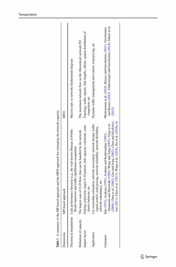
Note that in the literature, there is another line of approach to estimate the network capacity based on the macroscopic fundamental diagram (MFD). Compared to the MFD approach, the approach in the above discussion can be referred to as mathematical pro-gramming (MP)-based approach, which concerns the development of MP formulation to estimate the network capacity. Table 1 summarizes these two approaches with respect to theoretical foundations, definitions of capacity, impact factors, application, and representa-tive literature.

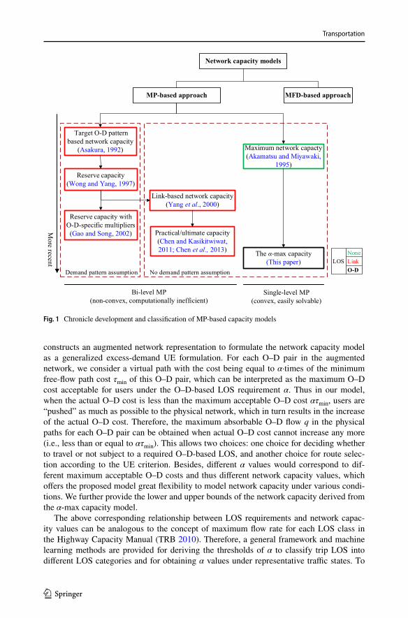
Based on Table 1, we can conclude that the theoretical foundations, the focus of defi-nition of network capacity, and the impact factors of these two approaches are differ-ent. Besides, there are both similarities and differences for the application of these two approaches. On the one hand, the applications of the MP-based approach focus on the long-term evaluation of network performance and network design, while the applications of the MFD approach consider the short-term assessment of dynamic traffic management and control. On the other hand, both can be used for traffic control and road pricing for different planning horizons (e.g., strategic planning versus operation planning). It should be noted that this paper focuses on the development of a single-level MP formulation for estimating the network capacity with trip level of service, which belongs to the MP-based approach. Figure  1 provides a brief summary and classification of MP-based network capacity models with respect to the MP formulation, the demand pattern assumption, and the LOS consideration.

Main contributions of this paper

To fill the research gap, this paper proposes the α-max capacity model by formulating the network capacity with the trip LOS consideration as a single-level MP. The proposed α-max capacity model estimates the maximum network capacity according to the require-ment of O–D-based LOS α. Specifically, using the concept of super-network, this model

Transportation

1 3

Tabl

e 1

A su

mm

ary

of th

e M

P-ba

sed

appr

oach

and

the

MFD

app

roac

h fo

r esti

mat

ing

the

netw

ork

capa

city

Dim

ensi

ons

MP-

base

d ap

proa

chM

FD

Theo

retic

al fo

unda

tions

Link

per

form

ance

func

tion

(e.g

., th

e w

ell-k

now

n B

urea

u of

Pub

lic

Road

s fun

ctio

n) a

nd tr

affic

equi

libriu

m a

ssig

nmen

tM

acro

scop

ic o

r net

wor

k fu

ndam

enta

l dia

gram

Defi

nitio

n of

cap

acity

The

larg

est s

um o

f O–D

flow

s tha

t can

be

hand

led

by th

e ne

twor

kTh

e m

axim

um n

etw

ork

flow

on

the

(theo

retic

al) n

etw

ork

FDIm

pact

fact

orPa

rkin

g re

stric

tion,

targ

et O

–D p

atte

rn, l

ink

capa

city

con

strai

nt, r

oute

ch

oice

beh

avio

r, et

cTo

polo

gy, t

raffi

c si

gnal

s, lin

k le

ngth

s, off

sets

, spa

tial d

istrib

utio

n of

co

nges

tion,

etc

App

licat

ion

Car

ow

ners

hip

estim

atio

n, n

etw

ork

asse

ssm

ent,

netw

ork

desi

gn, t

raffi

c si

gnal

con

trol,

road

pric

ing,

net

wor

k re

liabi

lity,

net

wor

k fle

xibi

lity,

ne

twor

k re

dund

ancy

, etc

Dyn

amic

traffi

c m

anag

emen

t and

con

trol,

road

pric

ing,

etc

Lite

ratu

reIid

a (1

972)

, Asa

kura

(199

2), A

saku

ra a

nd K

ashi

wad

ani (

1993

), A

kam

astu

and

Miy

awak

i (19

95),

Won

g an

d Ya

ng (1

997)

, Yan

g et

 al.

(200

0), C

hen

et a

l. (2

002)

, Gao

and

Son

g (2

002)

, Che

n an

d K

asik

itwi-

wat

(201

1), C

hen

et a

l. (2

013)

, Wan

g et

 al.

(201

8), X

u et

 al.

(201

8a, b

)

Maz

loum

ian

et a

l. (2

010)

, Boy

acı a

nd G

erol

imin

is (2

011)

, Ger

olim

inis

an

d B

oyac

ı (20

12),

Yild

irim

oglu

and

Ger

olim

inis

(201

4), S

aber

i et a

l. (2

015)

Transportation

1 3

constructs an augmented network representation to formulate the network capacity model as a generalized excess-demand UE formulation. For each O–D pair in the augmented network, we consider a virtual path with the cost being equal to α·times of the minimum free-flow path cost τmin of this O–D pair, which can be interpreted as the maximum O–D cost acceptable for users under the O–D-based LOS requirement α. Thus in our model, when the actual O–D cost is less than the maximum acceptable O–D cost ατmin, users are “pushed” as much as possible to the physical network, which in turn results in the increase of the actual O–D cost. Therefore, the maximum absorbable O–D flow q in the physical paths for each O–D pair can be obtained when actual O–D cost cannot increase any more (i.e., less than or equal to ατmin). This allows two choices: one choice for deciding whether to travel or not subject to a required O–D-based LOS, and another choice for route selec-tion according to the UE criterion. Besides, different α values would correspond to dif-ferent maximum acceptable O–D costs and thus different network capacity values, which offers the proposed model great flexibility to model network capacity under various condi-tions. We further provide the lower and upper bounds of the network capacity derived from the α-max capacity model.

The above corresponding relationship between LOS requirements and network capac-ity values can be analogous to the concept of maximum flow rate for each LOS class in the Highway Capacity Manual (TRB 2010). Therefore, a general framework and machine learning methods are provided for deriving the thresholds of α to classify trip LOS into different LOS categories and for obtaining α values under representative traffic states. To

Maximum network capacty(Akamatsu and Miyawaki,

1995)Reserve capacity

(Wong and Yang, 1997)

Link-based network capacity(Yang et al., 2000)

Practical/ultimate capacity(Chen and Kasikitwiwat,2011; Chen et al., 2013)

Target O-D pattern based network capacity

(Asakura, 1992)

Reserve capacity with O-D-specific multipliers(Gao and Song, 2002)

MP-based approach

Single-level MP(convex, easily solvable)

Bi-level MP(non-convex, computationally inefficient)

More recent

The -max capacity(This paper)

Demand pattern assumption No demand pattern assumption

MFD-based approach

Network capacity models

NoneLinkO-D

LOS

Fig. 1 Chronicle development and classification of MP-based capacity models

Transportation

1 3

solve the proposed α-max capacity model, a modified gradient projection algorithm with soft constraint technique is developed. The soft constraint technique always guarantees the feasible solution because the penalization of violating side constraints is imposed in the objective function without destroying the Cartesian product structure of the feasible set (Patriksson 2004, 2015; Nie et al. 2004). Numerical examples using an illustrative network and a realistic large-scale network are also presented to demonstrate the features of the pro-posed model as well as the applicability of the solution algorithm for large-scale network applications.

In summary, compared to the existing network capacity models, the features of the pro-posed model are threefold: (a) it considers trip LOS, which offers great flexibility to esti-mate the network capacity ranging from zero1 to the physical capacity including reserve, practical and ultimate capacities; (b) trip LOS can intuitively reflect users’ maximum acceptable O–D travel cost and also answer planners’ question about what is the network capacity under a certain O–D-based LOS requirement; and (c) it is a convex and tractable single-level MP, which is convenient for developing a computationally efficient solution algorithm for large-scale network applications.

The remainder of this paper is organized as follows. Section “Illustration of the mod-eling idea” illustrates our modeling idea of network capacity. The proposed α-max capac-ity model and discussions of its properties are provided in “The α-max network capacity model” section. Section “Solution algorithm” presents the solution algorithm. Numerical examples and conclusions are summarized in “Numerical examples” and “Concluding remarks” sections, respectively.

Illustration of the modeling idea

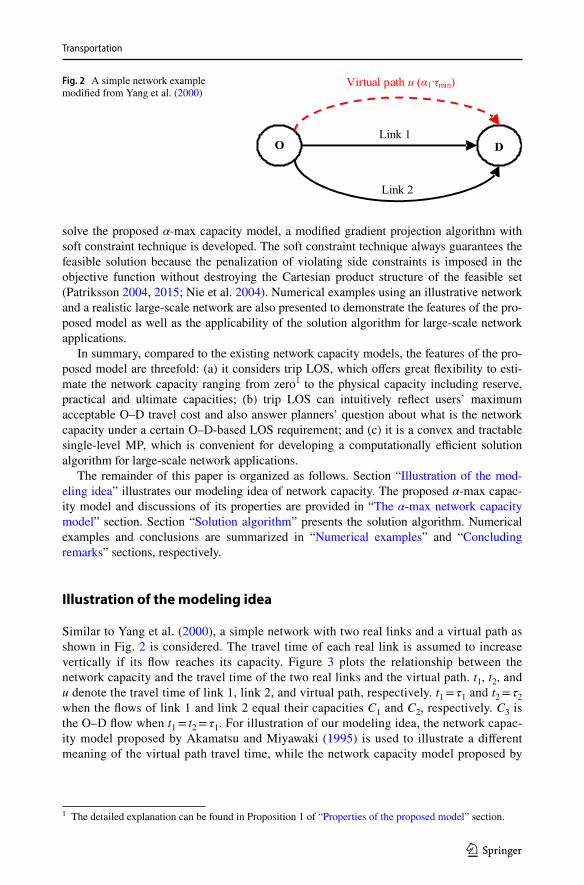
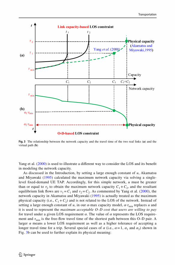
Similar to Yang et al. (2000), a simple network with two real links and a virtual path as shown in Fig. 2 is considered. The travel time of each real link is assumed to increase vertically if its flow reaches its capacity. Figure  3 plots the relationship between the network capacity and the travel time of the two real links and the virtual path. t1, t2, and u denote the travel time of link 1, link 2, and virtual path, respectively. t1 = τ1 and t2 = τ2 when the flows of link 1 and link 2 equal their capacities C1 and C2, respectively. C3 is the O–D flow when t1 = t2 = τ1. For illustration of our modeling idea, the network capac-ity model proposed by Akamatsu and Miyawaki (1995) is used to illustrate a different meaning of the virtual path travel time, while the network capacity model proposed by

Fig. 2 A simple network example modified from Yang et al. (2000)

Link 1O D

Link 2

Virtual path u ( 1· min)

1 The detailed explanation can be found in Proposition 1 of “Properties of the proposed model” section.

Transportation

1 3

Yang et al. (2000) is used to illustrate a different way to consider the LOS and its benefit in modeling the network capacity.

As discussed in the Introduction, by setting a large enough constant of u, Akamatsu and Miyawaki (1995) calculated the maximum network capacity via solving a single-level fixed-demand UE TAP. Accordingly, for this simple network, u must be greater than or equal to τ2 to obtain the maximum network capacity C1 + C2, and the resultant equilibrium link flows are v1 = C1 and v2 = C2. As commented by Yang et al. (2000), the network capacity in Akamatsu and Miyawaki (1995) is actually treated as the maximum physical capacity (i.e., C1 + C2) and is not related to the LOS of the network. Instead of setting a large enough constant of u, in our α-max capacity model, α·τmin replaces u and it is used to represent the maximum acceptable O–D cost that users are willing to pay for travel under a given LOS requirement α. The value of α represents the LOS require-ment and τmin is the free-flow travel time of the shortest path between this O–D pair. A larger α means a lower LOS requirement as well as a higher tolerance of accepting a longer travel time for a trip. Several special cases of α (i.e., α = 1, α1 and α2) shown in Fig. 3b can be used to further explain its physical meaning:

(a)

Capacity

t 1

C1

t Link capacity-based LOS constraint

Physical capacity(Akamatsu and

Miyawaki,1995)

O-D-based LOS constraint

Network capacity

Physical capacityt

2· min

min

min

2

1

t 2

1· min

C2 C3 C1+C2

Yang et al. (2000)

(b)

Fig. 3 The relationship between the network capacity and the travel time of the two real links (a) and the virtual path (b)

Transportation

1 3

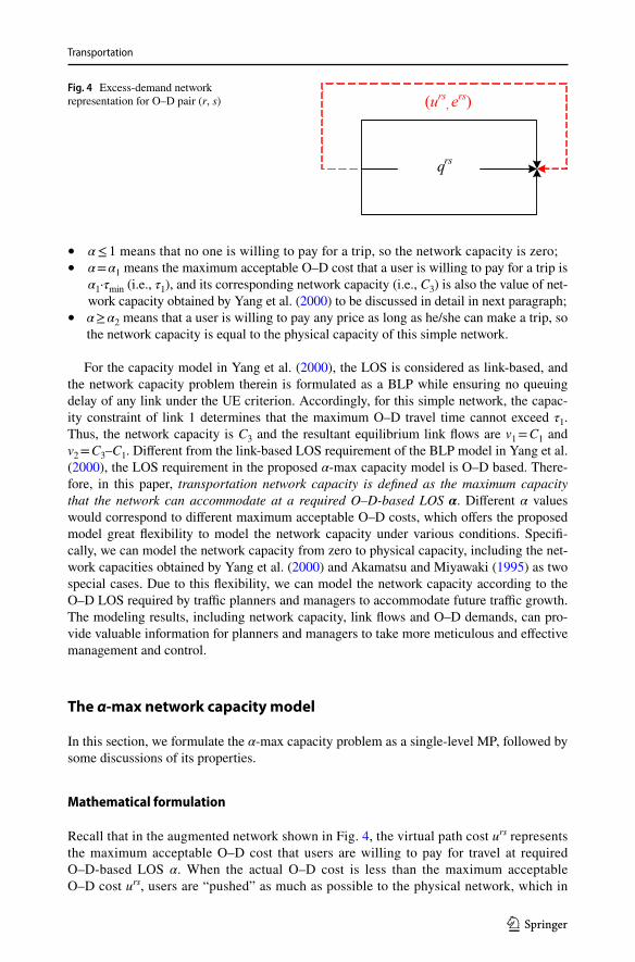
• α ≤ 1 means that no one is willing to pay for a trip, so the network capacity is zero;• α = α1 means the maximum acceptable O–D cost that a user is willing to pay for a trip is

α1·τmin (i.e., τ1), and its corresponding network capacity (i.e., C3) is also the value of net-work capacity obtained by Yang et al. (2000) to be discussed in detail in next paragraph;

• α ≥ α2 means that a user is willing to pay any price as long as he/she can make a trip, so the network capacity is equal to the physical capacity of this simple network.

For the capacity model in Yang et al. (2000), the LOS is considered as link-based, and the network capacity problem therein is formulated as a BLP while ensuring no queuing delay of any link under the UE criterion. Accordingly, for this simple network, the capac-ity constraint of link 1 determines that the maximum O–D travel time cannot exceed τ1. Thus, the network capacity is C3 and the resultant equilibrium link flows are v1 = C1 and v2 = C3–C1. Different from the link-based LOS requirement of the BLP model in Yang et al. (2000), the LOS requirement in the proposed α-max capacity model is O–D based. There-fore, in this paper, transportation network capacity is defined as the maximum capacity that the network can accommodate at a required O–D-based LOS α. Different α values would correspond to different maximum acceptable O–D costs, which offers the proposed model great flexibility to model the network capacity under various conditions. Specifi-cally, we can model the network capacity from zero to physical capacity, including the net-work capacities obtained by Yang et al. (2000) and Akamatsu and Miyawaki (1995) as two special cases. Due to this flexibility, we can model the network capacity according to the O–D LOS required by traffic planners and managers to accommodate future traffic growth. The modeling results, including network capacity, link flows and O–D demands, can pro-vide valuable information for planners and managers to take more meticulous and effective management and control.

The α‑max network capacity model

In this section, we formulate the α-max capacity problem as a single-level MP, followed by some discussions of its properties.

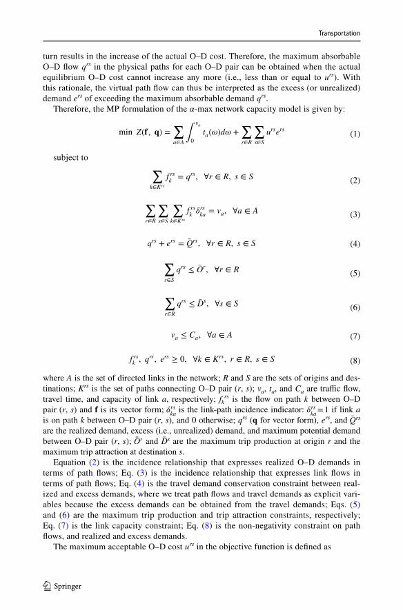
Mathematical formulation

Recall that in the augmented network shown in Fig. 4, the virtual path cost urs represents the maximum acceptable O–D cost that users are willing to pay for travel at required O–D-based LOS α. When the actual O–D cost is less than the maximum acceptable O–D cost urs, users are “pushed” as much as possible to the physical network, which in

Fig. 4 Excess-demand network representation for O–D pair (r, s)

qrs

(urs, ers)

Transportation

1 3

turn results in the increase of the actual O–D cost. Therefore, the maximum absorbable O–D flow qrs in the physical paths for each O–D pair can be obtained when the actual equilibrium O–D cost cannot increase any more (i.e., less than or equal to urs). With this rationale, the virtual path flow can thus be interpreted as the excess (or unrealized) demand ers of exceeding the maximum absorbable demand qrs.

Therefore, the MP formulation of the α-max network capacity model is given by:

subject to

where A is the set of directed links in the network; R and S are the sets of origins and des-tinations; Krs is the set of paths connecting O–D pair (r, s); va, ta, and Ca are traffic flow, travel time, and capacity of link a, respectively; fkrs is the flow on path k between O–D pair (r, s) and f is its vector form; �rs

ka is the link-path incidence indicator: �rs

ka = 1 if link a

is on path k between O–D pair (r, s), and 0 otherwise; qrs (q for vector form), ers, and Qrs are the realized demand, excess (i.e., unrealized) demand, and maximum potential demand between O–D pair (r, s); Or and Ds are the maximum trip production at origin r and the maximum trip attraction at destination s.

Equation  (2) is the incidence relationship that expresses realized O–D demands in terms of path flows; Eq.  (3) is the incidence relationship that expresses link flows in terms of path flows; Eq. (4) is the travel demand conservation constraint between real-ized and excess demands, where we treat path flows and travel demands as explicit vari-ables because the excess demands can be obtained from the travel demands; Eqs. (5) and (6) are the maximum trip production and trip attraction constraints, respectively; Eq.  (7) is the link capacity constraint; Eq.  (8) is the non-negativity constraint on path flows, and realized and excess demands.

The maximum acceptable O–D cost urs in the objective function is defined as

(1)min Z(� , �) =∑a∈A

∫va

0

ta(�)d� +∑r∈R

∑s∈S

ursers

(2)∑k∈Krs

f rsk

= qrs, ∀r ∈ R, s ∈ S

(3)∑r∈R

∑s∈S

∑k∈Krs

f rsk�rska

= va, ∀a ∈ A

(4)qrs + ers = Qrs, ∀r ∈ R, s ∈ S

(5)∑s∈S

qrs ≤ Or, ∀r ∈ R

(6)∑r∈R

qrs ≤ Ds, ∀s ∈ S

(7)va ≤ Ca, ∀a ∈ A

(8)f rsk, qrs, ers ≥ 0, ∀k ∈ Krs, r ∈ R, s ∈ S

Transportation

1 3

where αrs is the O–D-specific constant value of representing the required LOS between O–D pair (r, s). Specifically, �rs

min= mink∈Krs

{�rsk

} and �rs

k is the free-flow travel time of

path k between O–D pair (r, s), i.e., �rsk=∑

a∈A t0a�rska

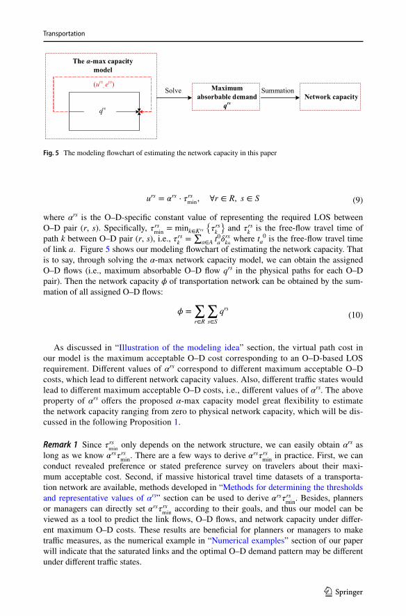
where ta0 is the free-flow travel time of link a. Figure 5 shows our modeling flowchart of estimating the network capacity. That is to say, through solving the α-max network capacity model, we can obtain the assigned O–D flows (i.e., maximum absorbable O–D flow qrs in the physical paths for each O–D pair). Then the network capacity � of transportation network can be obtained by the sum-mation of all assigned O–D flows:

As discussed in “Illustration of the modeling idea” section, the virtual path cost in our model is the maximum acceptable O–D cost corresponding to an O–D-based LOS requirement. Different values of αrs correspond to different maximum acceptable O–D costs, which lead to different network capacity values. Also, different traffic states would lead to different maximum acceptable O–D costs, i.e., different values of αrs. The above property of αrs offers the proposed α-max capacity model great flexibility to estimate the network capacity ranging from zero to physical network capacity, which will be dis-cussed in the following Proposition 1.

Remark 1 Since �rsmin

only depends on the network structure, we can easily obtain αrs as long as we know �rs�rs

min . There are a few ways to derive �rs�rs

min in practice. First, we can

conduct revealed preference or stated preference survey on travelers about their maxi-mum acceptable cost. Second, if massive historical travel time datasets of a transporta-tion network are available, methods developed in “Methods for determining the thresholds and representative values of αrs” section can be used to derive �rs�rs

min . Besides, planners

or managers can directly set �rs�rsmin

according to their goals, and thus our model can be viewed as a tool to predict the link flows, O–D flows, and network capacity under differ-ent maximum O–D costs. These results are beneficial for planners or managers to make traffic measures, as the numerical example in “Numerical examples” section of our paper will indicate that the saturated links and the optimal O–D demand pattern may be different under different traffic states.

(9)urs = �rs⋅ �rs

min, ∀r ∈ R, s ∈ S

(10)� =∑r∈R

∑s∈S

qrs

qrs

(urs, ers)

The -max capacity model

Maximum absorbable demand

qrsNetwork capacity

Solve Summation

Fig. 5 The modeling flowchart of estimating the network capacity in this paper

Transportation

1 3

Properties of the proposed model

As discussed above, the α-max capacity model has great flexibility to model the net-work capacity under various conditions due to the consideration of O–D-based LOS. This great flexibility is mathematically defined by Proposition 1.

Proposition 1 The lower bound and the upper bound of network capacity obtained by the proposed α-max capacity model are zero and the physical capacity of transportation network, respectively.

Proof In the proposed model, when αrs = 1, it means that the maximum acceptable O–D cost for every O–D pair is equal to the minimum free-flow travel time. Therefore, the flow of each O–D pair should be zero in order to ensure the free-flow state, thus leading to zero as the lower bound of network capacity defined in the proposed model, i.e., �min = 0 . Recall the excess-demand network representation in Fig.  4, if αrs is a sufficiently large enough value, users are pushed to the physical routes as much as possible until the physical network reaches its physical maximum capacity. In fact, the network capacity under this condition can be derived by solving the maximum flow problem in graph theory, which has no travel choice behavior component. Consequently, the upper bound of network capacity will be the physical capacity, i.e., �max = �physical . This completes the proof. □

Remark 2 Too small or too large value of network capacity has limited meaning for plan-ners or managers from the practical point of view. In fact, compared with the continuous LOS, LOS categories could provide useful and important information to planners and man-agers. For example, typical practice is to design traffic facilities such as highway or pedes-trians facilities to operate at LOS C or D (TRB 2010). Besides, planners and managers also pay more attention to network performance under some representative traffic states, such as commuting peak and off-peak. Then, two questions naturally arise: (1) similar to the classification of highway LOS (TRB, 2010), can we derive thresholds of αrs to classify the trip LOS into different categories? and (2) can we get values of αrs corresponding to some representative traffic states? Sect. “Methods for determining the thresholds and representa-tive values of αrs” will introduce methods to obtain the thresholds and representative values of αrs.

Proposition 2 The α-max network capacity model is equivalent to two behavioral choices: one choice for deciding whether to travel or not subject to a required O–D-based LOS, and another choice for route selection according to the user equilibrium criterion.

Proof First of all, we examine the Karush–Kukn–Tucker (KKT) conditions of the proposed model. As excess demands can be obtained from the travel demands via Eq. (4), we treat path flows and travel demands as explicit variables. We only attach Lagrangian multipliers πrs, mr, ns, and da to Eqs. (2), (5), (6) and (7), respectively, given that Eqs. (3)–(4) are the definitional constraints with respect to link flows and travel demands. Then, the Lagrangian function of the proposed model and its first-order partial derivatives with respect to path flows and travel demands can be expressed as:

(11)� ∈[0, �physical

]

Transportation

1 3

where crsk=∑

a∈A ta�va��rska

is the travel time of path k between OD pair (r, s).□Therefore, the KKT conditions of the proposed α-max network capacity model with

respect to path flows and travel demands are thus:

Equations (15)–(16) are the equilibrium conditions for the capacitated UE problem, where da is interpreted as the link delay when the link flow reaches its capacity. These two equations indicate that the travel time (including delay) on any physical path connecting an O–D pair should equal the minimum-path travel time if the flow on this path is positive. If the flow on this path is zero, its travel time must be greater than or equal to the mini-mum travel time. Equations (17)–(18) have a similar interpretation. If qrs > 0, the general-ized O–D cost (πrs + mr + ns) for users equals the maximum acceptable O–D cost (urs) at the requirement of the O–D-based LOS α. If qrs = 0, then the generalized O–D cost for users is greater than the maximum O–D cost, which is too high to induce any O–D flow into the physical network. Eq. (19) is non-negativity constraint.

According to the KKT conditions of the proposed α-max network capacity model, Eqs. (17)–(18) are the mechanism for deciding whether to travel or not, while Eqs. (15)–(16) are the mechanism for route choice according to the user equilibrium criterion. This com-pletes proof. □

As can be seen from Eqs. (15)–(18), except for path travel time ckrs, each used physi-

cal path has an endogenous cost (i.e., mr + ns +∑

a∈A da�rska

) which consists of origin, destination, and delay penalty costs. Actually, this endogenous cost is the maximum

(12)

L(� , �, �, �, �, �) = Z(� , �) +∑r∈R

∑s∈S

𝜋rs

(qrs −

∑k∈Krs

f rsk

)

+∑r∈R

mr

(∑s∈S

qrs − Or

)+∑s∈S

ns

(∑r∈R

qrs − Ds

)+∑a∈A

da

(∑r∈R

∑s∈S

∑k∈Krs

f rsk𝛿rska− Ca

)

(13)�L

�f rsk

=∑a∈A

ta(va)�rska− �rs +

∑a∈A

da�rska

= crsk− �rs +

∑a∈A

da�rska

(14)�L

�qrs= −urs + �rs + mr + ns

(15)f rsk

(crsk+

∑a∈A

da�rska− �rs

)= 0, ∀k ∈ Krs, r ∈ R, s ∈ S

(16)crsk+

∑a∈A

da�rska− �rs ≥ 0, ∀k ∈ Krs, r ∈ R, s ∈ S

(17)qrs(�rs + mr + ns − urs

)= 0, ∀r ∈ R, s ∈ S

(18)�rs + mr + ns − urs ≥ 0, ∀r ∈ R, s ∈ S

(19)f rsk

≥ 0, qrs ≥ 0, ∀k ∈ Krs, r ∈ R, s ∈ S

Transportation

1 3

additional travel time that travelers are willing to pay for fulfilling the purpose of reach-ing the destination, which has an upper bound given by Proposition 3.

Proposition 3 The requirement of a specified trip LOS makes each route between each O–D pair have an endogenous cost beyond the path travel time, which is upper bounded by

Proof Given any O–D pair, the optimality conditions in Eqs. (15)–(18) indicate that all the used routes have

Since urs − crsk≤ urs − �rs

min , we have mr + ns +

∑a∈A

da�rska

≤ (�rs − 1)�rsmin

. This completes

the proof. □

Below we examine the uniqueness issue of the proposed model. Compared with the classical excess demand formulation (Beckman et al. 1956; Sheffi 1985), the three addi-tional constraints [i.e., Eqs. (5)–(7)] are all linear, and the constant virtual path cost urs replaces the elastic demand function for each O–D pair. Thus, the proposed model is still strictly convex with respect to link flows, but linear with respect to O–D demands. This means that the uniqueness of the equilibrium links flows can be guaranteed, while the optimal O–D demands may not be unique. In order to determine a unique optimal O–D demand, Akamatsu and Miyawaki (1995) selected the solution by minimizing the closeness of the O–D matrix to some target O–D pattern. To avoid embracing any refer-ence O–D pattern, we can add an entropy term of qrs directly into the objective function of Eq. (1):

where γ is the parameter that shall be set to a large enough value. Then, the second-order derivative of Z�(� , �) with respect to qrs is

In other words, the Hessian matrix in terms of qrs is positive definite, which means that the objective function is strictly convex with respect to qrs, and thus the optimal O–D demands can be determined uniquely. We should point out that the entropy term in Eq. (22) is added just for ensuring a unique solution of the optimal O–D demand, which is different from the entropy term in the combined trip distribution-assignment model. Besides, we can also use stochastic user equilibrium to replace the UE for obtaining a unique solution of the optimal O–D demand, which is however not the main focus of this paper.

(20)mr + ns +∑a∈A

da�rska

≤ (�rs − 1)�rsmin

(21)

⎧⎪⎨⎪⎩

crsk+

�a∈A

da�rska− �rs = 0

�rs + mr + ns − urs = 0

⇒ mr + ns +�a∈A

da�rska

= urs − crsk

(22)min Z�(� , �) =∑a∈A

∫va

0

ta(�)d� +1

�

∑r∈R

∑s∈S

qrs(ln qrs − 1) +∑r∈R

∑s∈S

ursers

(23)�2Z�(� , �)

�qrs�qmn=

{1

�qrsfor (r, s) = (m, n)

0 otherwise

Transportation

1 3

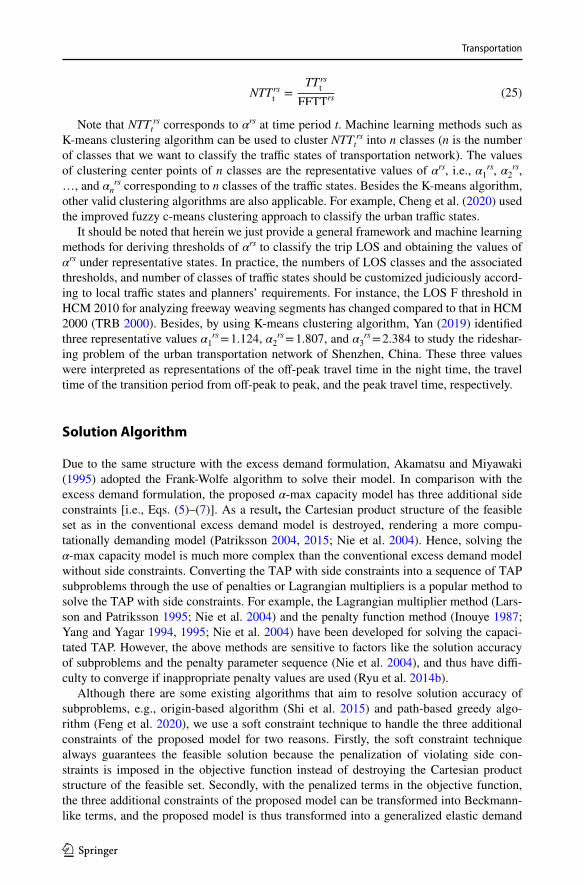
Methods for determining the thresholds and representative values of αrs

As the uncertainties of traffic supply and demand exist in the transportation network, traffic states between an O–D pair will not be unchanged, leading to travel time vari-ability. One can aggregate massive data of individual trips collected by sensors (e.g., floating cars) during a long-term period into travel time datasets (TTt

rs) by O–D pair (r, s) and time period t:

where o(i) and d(i) are the starting and ending points of trip i, respectively; z(r) is the geo-graphic region of zone r, ⌊�(i)⌋ is the rounded start time of trip i using the floor operator ⌊⋅⌋ . For simplicity, let �rs

min, �rs

�, and �rs

max denote the minimum travel time, ρ percentile of

travel time and maximum travel time in travel time datasets.First of all, we provide a general framework based on on-time arrival probability to

determine thresholds for classifying the trip LOS. The maximum acceptable O–D cost is the price that a traveler is willing to pay for travel, which actually depends on his/her requirement of on-time arrival probability. If the traveler requires a ρ on-time arrival probability (e.g., 80%), his/her maximum acceptable O–D cost must be greater than or equal to �rs

� , and the corresponding αrs is �rs

�∕�rs

min . Obviously, the on-time arrival prob-

ability of �rsmin

and �rsmax

are 0 and 100%, respectively. If we choose 50%, 80% as another two requirements of on-time arrival probability, we will have four thresholds of αrs (i.e., 1, �rs

50%∕�rs

min,�rs80%

∕�rsmin

, and �rsmax

∕�rsmin

) to classify the trip LOS and its correspond-ing capacity into four LOS classes from A to D as shown in Fig. 6. Compared with the highway LOS categories defined in the Highway Capacity Manual (HCM) 2010 (TRB 2010), we can have a similar interpretation of these O–D-based LOS classes. For exam-ple, when �rs ∈

(�rs80%

∕�rsmin

, �rsmax

∕�rsmin

] , the transportation network can provide LOS C

of network capacity, and the maximum network capacity under LOS C is the network capacity corresponding to �rs = �rs

max∕�rs

min . In fact, this network capacity is the maxi-

mum physical amount of flow that the network can accommodate, which is similar to the highway operational capacity defined by LOS E in HCM 2010.

Although the thresholds are useful in obtaining the range of network capacity under specified LOS class, the network capacities under some representative traffic states such as morning peak are also key concerns for planners and managers. Then, we can further use machine learning methods to obtain the values of αrs under representative states for refer-ence to planners and managers. Since αrs is dimensionless, the travel time datasets of all trips TTt

rs are normalized by the minimum free-flow travel time FFTTrs of O–D pair (r, s):

(24)TTrst= {i�o(i) ∈ z(r), d(i) ∈ z(s), ⌊�(i)⌋ = t}

Fig. 6 The illustration of O–D based LOS classes and network capacities

LOS αα

Net

wor

k ca

paci

ty

LOS A

1

LOS B

LOS C

LOS D

0

φ80%

φ50%

φphysical

τ rs50% /τ rs

min τ rs80%/τ rs

min τ rsmax/τ rs

min

Transportation

1 3

Note that NTTtrs corresponds to αrs at time period t. Machine learning methods such as

K-means clustering algorithm can be used to cluster NTTtrs into n classes (n is the number

of classes that we want to classify the traffic states of transportation network). The values of clustering center points of n classes are the representative values of αrs, i.e., α1

rs, α2rs,

…, and αnrs corresponding to n classes of the traffic states. Besides the K-means algorithm,

other valid clustering algorithms are also applicable. For example, Cheng et al. (2020) used the improved fuzzy c-means clustering approach to classify the urban traffic states.

It should be noted that herein we just provide a general framework and machine learning methods for deriving thresholds of αrs to classify the trip LOS and obtaining the values of αrs under representative states. In practice, the numbers of LOS classes and the associated thresholds, and number of classes of traffic states should be customized judiciously accord-ing to local traffic states and planners’ requirements. For instance, the LOS F threshold in HCM 2010 for analyzing freeway weaving segments has changed compared to that in HCM 2000 (TRB 2000). Besides, by using K-means clustering algorithm, Yan (2019) identified three representative values α1

rs = 1.124, α2rs = 1.807, and α3

rs = 2.384 to study the rideshar-ing problem of the urban transportation network of Shenzhen, China. These three values were interpreted as representations of the off-peak travel time in the night time, the travel time of the transition period from off-peak to peak, and the peak travel time, respectively.

Solution Algorithm

Due to the same structure with the excess demand formulation, Akamatsu and Miyawaki (1995) adopted the Frank-Wolfe algorithm to solve their model. In comparison with the excess demand formulation, the proposed α-max capacity model has three additional side constraints [i.e., Eqs. (5)–(7)]. As a result, the Cartesian product structure of the feasible set as in the conventional excess demand model is destroyed, rendering a more compu-tationally demanding model (Patriksson 2004, 2015; Nie et al. 2004). Hence, solving the α-max capacity model is much more complex than the conventional excess demand model without side constraints. Converting the TAP with side constraints into a sequence of TAP subproblems through the use of penalties or Lagrangian multipliers is a popular method to solve the TAP with side constraints. For example, the Lagrangian multiplier method (Lars-son and Patriksson 1995; Nie et al. 2004) and the penalty function method (Inouye 1987; Yang and Yagar 1994, 1995; Nie et al. 2004) have been developed for solving the capaci-tated TAP. However, the above methods are sensitive to factors like the solution accuracy of subproblems and the penalty parameter sequence (Nie et al. 2004), and thus have diffi-culty to converge if inappropriate penalty values are used (Ryu et al. 2014b).

Although there are some existing algorithms that aim to resolve solution accuracy of subproblems, e.g., origin-based algorithm (Shi et  al. 2015) and path-based greedy algo-rithm (Feng et al. 2020), we use a soft constraint technique to handle the three additional constraints of the proposed model for two reasons. Firstly, the soft constraint technique always guarantees the feasible solution because the penalization of violating side con-straints is imposed in the objective function instead of destroying the Cartesian product structure of the feasible set. Secondly, with the penalized terms in the objective function, the three additional constraints of the proposed model can be transformed into Beckmann-like terms, and the proposed model is thus transformed into a generalized elastic demand

(25)NTTrst=

TTrst

FFTTrs

Transportation

1 3

UE traffic assignment model. This means that we can use the existing widely used algo-rithms to solve the proposed α-max capacity model.

Specifically, the proposed model is rewritten as:

subject to Eqs. (2)–(4) and (8), where Or and Ds are the trip production at origin r and the trip attraction at destination s; and pr(·), ps(·), and pa(·) are the soft penalty functions for relaxing Eqs. (5)–(7), respectively.

The following exponential-form soft penalty function has been shown to successfully relax the hard capacity constraint in solving the capacitated TAP (Nguyen et al. 2001; Noh 2013; Ryu et al. 2017):

where θ is a parameter. We use the above exponential-form soft penalty function to relax the other two side constraints in Eqs. (5)–(6) of our proposed model.

In fact, pa, pr and ps in soft constraint technique are used to approximate the Lagrangian multipliers da, mr, and ns associated with Eqs. (7), (5) and (6). In other words, the path cost and O–D cost in the elastic demand UE traffic assignment model are respectively replaced by:

where krs is the shortest path of O–D pair (r, s).Therefore, the gradient projection algorithm developed by Ryu et  al. (2014a) for

solving the elastic demand TAP can be adopted to solve our proposed model along with the above soft constraint technique. In the modified gradient projection algorithm with soft constraint technique, the flow update per iteration is conducted as follows: (1) if the calculated O–D cost in iteration n is smaller than its corresponding virtual path cost, it means the O–D actual congestion level is lower than the maximum acceptable level and thus more O–D flows should be pushed into the physical network; and (2) if the O–D actual congestion level is higher than the maximum acceptable level, more O–D flows should be pushed into the virtual path. Three modifications are also made to the gradi-ent projection algorithm developed by Ryu et al. (2014a): (1) the second-order deriva-tive of the objective function in Eq. (26) with respect to the virtual path flow is zero because urs is a constant number rather than an excess demand function Wrs(.) as in Ryu

(26)

min Z(� , �) =∑a∈A

∫va

0

ta(�)d� +∑a∈A

∫va

0

pa(�)d� +∑r∈R

∑s∈S

ursers

+∑r∈R

∫Or

0

pr(�)d� +∑s∈S

∫Ds

0

ps(�)d�

(27)pa =xa

Ca

⋅ exp(� ⋅

(xa − Ca

))

(28)pr =

Or

Or ⋅ exp

(� ⋅

(Or − O

r))

ps =Ds

Ds ⋅ exp

(� ⋅

(Ds − D

s))

(29)gcrsk=∑a∈A

(ta(va)+ pa

(va))�rska, ∀k ∈ Krs, r ∈ R, s ∈ S

(30)g𝜋rs = gcrskrs

+ pr + ps, ∀r ∈ R, s ∈ S

Transportation

1 3

et  al. (2014a); (2) a new stopping criterion, i.e., the relative gap (RG)

RG =

∑r∈R

∑s∈S

∑k∈Krs

f rsk(n)

�gcrs

k(n)−gcrs

krs(n)(n)

�

∑r∈R

∑s∈S

∑k∈Krs

gcrsk(n)f rs

k(n)

≤ � , is used where n is the number of the increment

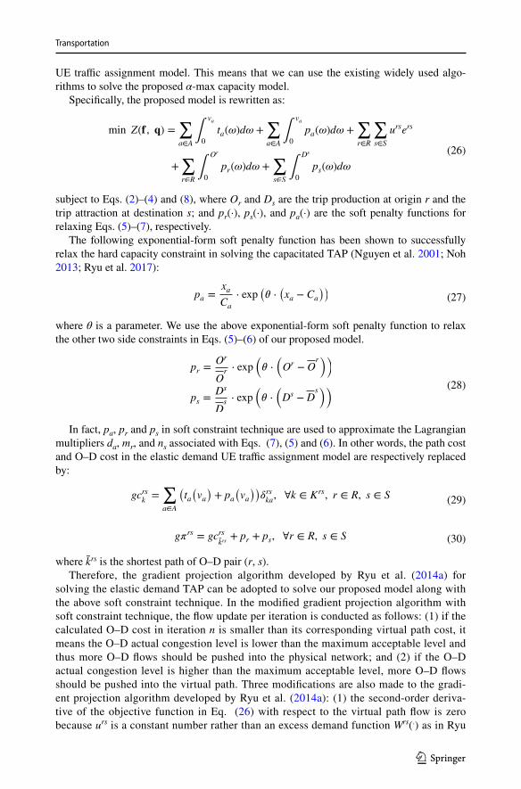
iteration of the algorithm; and (3) note that column generation is used to generate the shortest paths based on the current link travel times and augment the path set with new paths, so in the first iteration there is only one shortest path for each O–D pair and RG will be equal to zero. The overall flowchart of the modified gradient projection algo-rithm with soft constraint technique is shown in Fig. 7, and its detailed solution proce-dure is as follows:

Convergence ?

Results: network capacity

g rs(n) urs

Yes

No

Yes

No

Column generation• Increment iteration counter: n = n + 1• Update link, path and O-D costs: gta (n), , g rs(n)• Update path set by solving shortest path: Krs(n)

( )rskgc n

Update flow by decreasing demand with urs

•

•

•

( ) ( )( )rs

rsrs rsk

k K n

e n Q f n∈

= − ∑

( ) ( ) ( ) ( )( )max 1 , 0rs rs rs rskk rsf n f n g n u

nκ π

ψ = − − −

( ) ( ) ( ) ( )( )( )

11rs

rs rs rsa a k k ka

k K n

v n v n f n f n δ∈

= − + − −∑

Initialization( ) ( ) ( ) ( ), 0 0, 0, 0, ,

rsrs rs rs rsk af n v n e n Q qu n n= = == =

Update flow by increasing demand with

•

•

•

•

( ) ( ) ( ) ( ) ( )( )max 1 , 0rsrs rs rs rs

rs k ne n e n u gc n

nκ

ψ = − − −

( ) ( ) ( ) ( ) ( ) ( )( )max 1 , 0rsrs rs rs rs

kkk rs k nk

f n f n gc n gc nn

κψ

= − − −

( ) ( ) ( )( )( )

( )rsrs

rs

rsrs rs rskk n

k K nk k n

f n Q f n e n∈≠

= − −∑

( ) ( ) ( ) ( )( )( )

11rs

rs rs rsa a k k ka

k K n

v n v n f n f n δ∈

= − + − −∑

( )rsrsk n

gc

Fig. 7 Flowchart of the modified gradient projection algorithm with soft constraint technique for solving the proposed model

Transportation

1 3

Transportation

1 3

Numerical examples

In this section, two networks are used to illustrate the features and applicability of the proposed model. For the parameters used in the models, we use a unified α for all O–D pairs for simplicity, although the parameter αrs should be O–D pair specific. The maximum potential travel demands Qrs are assumed to be 2 times of the current O–D demands, and the maximum trip production Or and attraction Ds are assumed to be 1.8 times of the cur-rent trip production and attraction. For the parameters used in the solution algorithm, the parameter θ in the soft penalty function is set as 1. The step size κ is 0.4. The tolerance error for the stopping criterion (RG) is set at 1E-6. The solution algorithm is coded in Intel Visual FORTRAN XE, and run on a 3.40 GHz processor with 16.00 GB of RAM.

Example 1: grid network

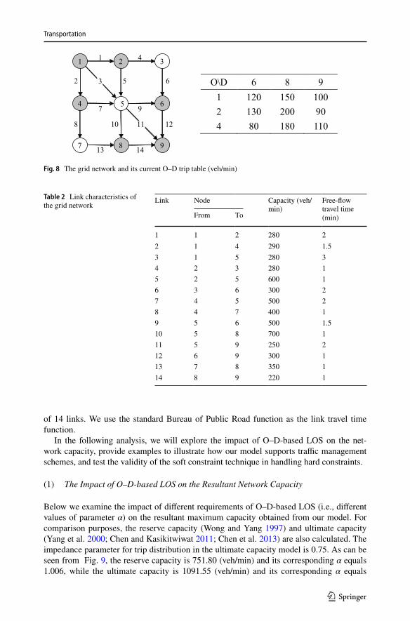
The grid network as depicted in Fig. 8 consists of 9 nodes, 14 directed links, and 9 O–D pairs. Nodes 1, 2, and 4 are origin nodes; while nodes 6, 8, and 9 are destination nodes (all shaded). The current O–D trip table is also given in Fig. 8. Table 2 gives the characteristics

Transportation

1 3

of 14 links. We use the standard Bureau of Public Road function as the link travel time function.

In the following analysis, we will explore the impact of O–D-based LOS on the net-work capacity, provide examples to illustrate how our model supports traffic management schemes, and test the validity of the soft constraint technique in handling hard constraints.

(1) The Impact of O–D-based LOS on the Resultant Network Capacity

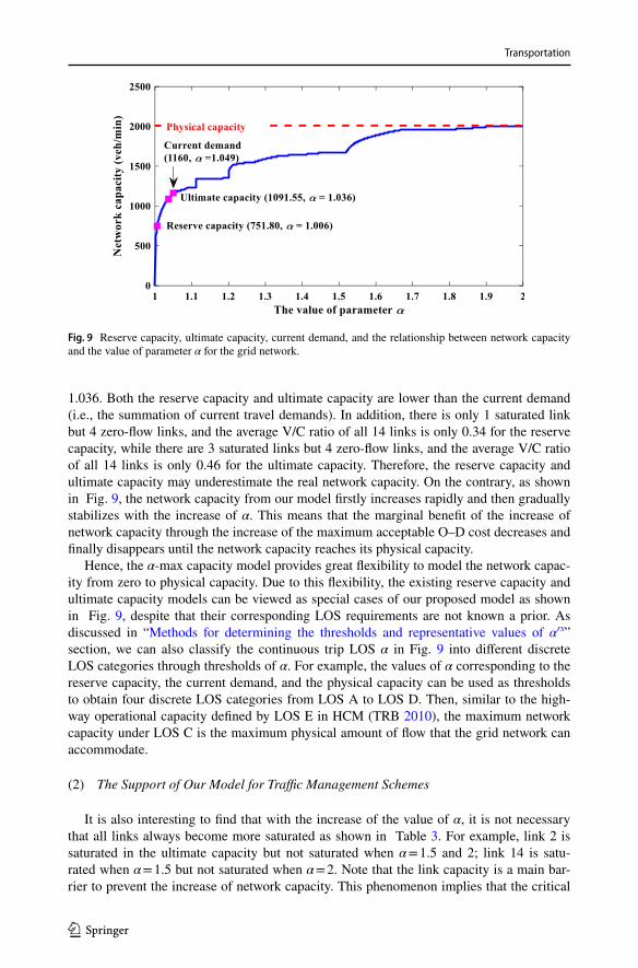
Below we examine the impact of different requirements of O–D-based LOS (i.e., different values of parameter α) on the resultant maximum capacity obtained from our model. For comparison purposes, the reserve capacity (Wong and Yang 1997) and ultimate capacity (Yang et al. 2000; Chen and Kasikitwiwat 2011; Chen et al. 2013) are also calculated. The impedance parameter for trip distribution in the ultimate capacity model is 0.75. As can be seen from Fig. 9, the reserve capacity is 751.80 (veh/min) and its corresponding α equals 1.006, while the ultimate capacity is 1091.55 (veh/min) and its corresponding α equals

1 3

4

7

5

9

2

6

8

1 4

7 9

13 14

2

8

5

10

6

12

3

11

O\D 6 8 91 120 150 1002 130 200 904 80 180 110

Fig. 8 The grid network and its current O–D trip table (veh/min)

Table 2 Link characteristics of the grid network

Link Node Capacity (veh/min)

Free-flow travel time (min)From To

1 1 2 280 22 1 4 290 1.53 1 5 280 34 2 3 280 15 2 5 600 16 3 6 300 27 4 5 500 28 4 7 400 19 5 6 500 1.510 5 8 700 111 5 9 250 212 6 9 300 113 7 8 350 114 8 9 220 1

Transportation

1 3

1.036. Both the reserve capacity and ultimate capacity are lower than the current demand (i.e., the summation of current travel demands). In addition, there is only 1 saturated link but 4 zero-flow links, and the average V/C ratio of all 14 links is only 0.34 for the reserve capacity, while there are 3 saturated links but 4 zero-flow links, and the average V/C ratio of all 14 links is only 0.46 for the ultimate capacity. Therefore, the reserve capacity and ultimate capacity may underestimate the real network capacity. On the contrary, as shown in Fig. 9, the network capacity from our model firstly increases rapidly and then gradually stabilizes with the increase of α. This means that the marginal benefit of the increase of network capacity through the increase of the maximum acceptable O–D cost decreases and finally disappears until the network capacity reaches its physical capacity.

Hence, the α-max capacity model provides great flexibility to model the network capac-ity from zero to physical capacity. Due to this flexibility, the existing reserve capacity and ultimate capacity models can be viewed as special cases of our proposed model as shown in Fig. 9, despite that their corresponding LOS requirements are not known a prior. As discussed in “Methods for determining the thresholds and representative values of αrs” section, we can also classify the continuous trip LOS α in Fig.  9 into different discrete LOS categories through thresholds of α. For example, the values of α corresponding to the reserve capacity, the current demand, and the physical capacity can be used as thresholds to obtain four discrete LOS categories from LOS A to LOS D. Then, similar to the high-way operational capacity defined by LOS E in HCM (TRB 2010), the maximum network capacity under LOS C is the maximum physical amount of flow that the grid network can accommodate.

(2) The Support of Our Model for Traffic Management Schemes

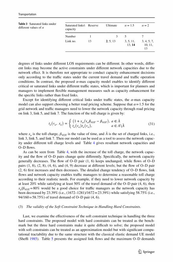
It is also interesting to find that with the increase of the value of α, it is not necessary that all links always become more saturated as shown in Table 3. For example, link 2 is saturated in the ultimate capacity but not saturated when α = 1.5 and 2; link 14 is satu-rated when α = 1.5 but not saturated when α = 2. Note that the link capacity is a main bar-rier to prevent the increase of network capacity. This phenomenon implies that the critical

Fig. 9 Reserve capacity, ultimate capacity, current demand, and the relationship between network capacity and the value of parameter α for the grid network.

Transportation

1 3

degrees of links under different LOS requirements can be different. In other words, differ-ent links may become the active constraints under different network capacities due to the network effect. It is therefore not appropriate to conduct capacity enhancement decisions only according to the traffic states under the current travel demand and traffic operation conditions. In contrast, the proposed α-max capacity model enables to identify different critical or saturated links under different traffic states, which is important for planners and managers to implement flexible management measures such as capacity enhancement for the specific links rather than fixed links.

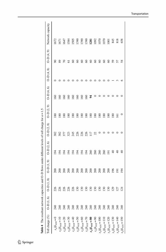
Except for identifying different critical links under traffic states, the α-max capacity model can also support choosing a better road pricing scheme. Suppose that α = 1.5 for the grid network and traffic managers need to lower the network capacity through road pricing on link 3, link 5, and link 7. The function of the toll charge is given by:

where xa is the toll charge, βVOT is the value of time, and A is the set of charged links, i.e., link 3, link 5, and link 7. Then our model can be used as a tool to assess the network capac-ity under different toll charge levels and Table 4 gives resultant network capacities and O–D flows.

As can be seen from Table 4, with the increase of the toll charge, the network capac-ity and the flow of O–D pairs change quite differently. Specifically, the network capacity generally decreases. The flow of O–D pair (1, 6) keeps unchanged; while flows of O–D pairs (1, 8), (2, 8), (4, 6), and (4, 9) decrease at different levels; but the flow of O–D pair (2, 6) first increases and then decreases. The detailed change tendency of O–D flows, link flows and network capacity enables traffic managers to determine a reasonable toll charge according to their realistic needs. For example, if they need to lower network capacity by at least 20% while satisfying at least 50% of the travel demand of the O–D pair (4, 6), then xa/βVOT = 80% would be a good choice for traffic managers as the network capacity has been decreased by 23.39% (i.e., (1672–1281)/1672 = 23.39%) while satisfying 58.75% (i.e., 94/160 = 58.75%) of travel demand of O–D pair (4, 6).

(3) The validity of the Soft Constraint Technique in Handling Hard Constraints.

Last, we examine the effectiveness of the soft constraint technique in handling the three hard constraints. The proposed model with hard constraints can be treated as the bench-mark but the three hard constraints make it quite difficult to solve; the proposed model with soft constraints can be treated as an approximation model but with significant compu-tational tractability due to the same structure with the classical elastic demand UE model (Sheffi 1985). Table 5 presents the assigned link flows and the maximum O–D demands

(31)ta(va, xa

)=

{ (1 + xa∕xa𝛽VOT − 𝛽VOT

), a ∈ A

ta(va)ta(va), a ∈ A�A

Table 3 Saturated links under different values of α

Saturated links\capacity

Reserve Ultimate α = 1.5 α = 2

Number 1 3 5 7Link no. 13 2, 5, 13 3, 5, 11,

13, 143, 4, 5, 7,

10, 11, 13

Transportation

1 3

Tabl

e 4

The

resu

ltant

net

wor

k ca

paci

ties a

nd O

–D fl

ows u

nder

diff

eren

t lev

els o

f tol

l cha

rge

for α

= 1.

5

Toll

char

ge (%

)O

–D (1

, 6)

O–D

(1, 8

)O

–D (1

, 9)

O–D

(2, 6

)O

–D (2

, 8)

O–D

(2, 9

)O

–D (4

, 6)

O–D

(4, 8

)O

–D (4

, 9)

Net

wor

k ca

paci

ty

x a/β

VO

T = 0

240

226

200

194

382

180

160

090

1672

x a/β

VO

T = 10

240

226

200

194

382

180

160

089

1671

x a/β

VO

T = 20

240

226

200

194

377

180

160

070

1647

x a/β

VO

T = 30

240

226

200

194

323

180

160

061

1584

x a/β

VO

T = 40

240

226

200

194

245

180

160

060

1505

x a/β

VO

T = 50

240

130

200

194

226

180

160

060

1390

x a/β

VO

T = 60

240

130

200

194

226

180

160

060

1390

x a/β

VO

T = 70

240

130

200

194

226

180

160

060

1390

x a/β

VOT =

8024

013

020

026

011

718

094

060

1281

x a/β

VO

T = 90

240

130

200

260

2218

00

060

1092

x a/β

VO

T = 10

024

013

020

026

00

180

00

6010

70x a

/βV

OT =

110

240

130

200

260

018

00

060

1070

x a/β

VO

T = 12

024

013

020

019

10

180

00

6010

01x a

/βV

OT =

130

240

129

196

400

180

01

5984

5x a

/βV

OT =

140

240

127

191

400

161

03

5781

8x a

/βV

OT =

150

240

124

194

400

00

654

658

Transportation

1 3

obtained from the proposed models with hard constraints and soft constraints, respectively. One can see that the results from the proposed models with hard constraints and soft con-straints are quite close with the maximum error of 1.95% for link volumes and 3.04% for maximum O–D demands. Therefore, the soft constraint technique can have a high-quality accuracy in handling hard constraints while ensuring the existence of a feasible solution and computational efficiency. Next section will further test the efficiency of the soft con-straint technique in handling the three hard constraints for large-scale network application.

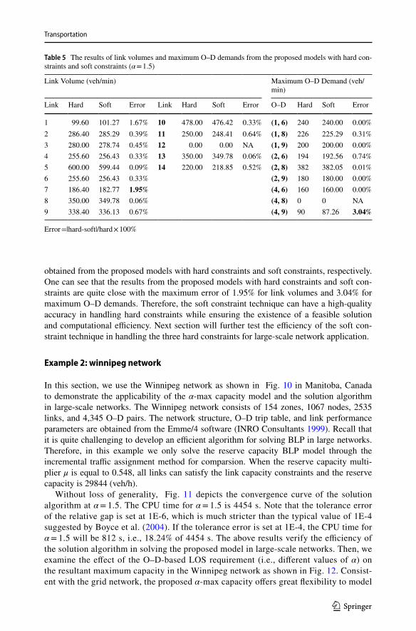
Example 2: winnipeg network

In this section, we use the Winnipeg network as shown in Fig. 10 in Manitoba, Canada to demonstrate the applicability of the α-max capacity model and the solution algorithm in large-scale networks. The Winnipeg network consists of 154 zones, 1067 nodes, 2535 links, and 4,345 O–D pairs. The network structure, O–D trip table, and link performance parameters are obtained from the Emme/4 software (INRO Consultants 1999). Recall that it is quite challenging to develop an efficient algorithm for solving BLP in large networks. Therefore, in this example we only solve the reserve capacity BLP model through the incremental traffic assignment method for comparsion. When the reserve capacity multi-plier μ is equal to 0.548, all links can satisfy the link capacity constraints and the reserve capacity is 29844 (veh/h).

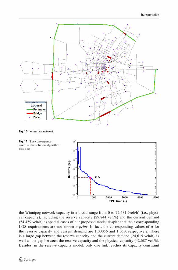
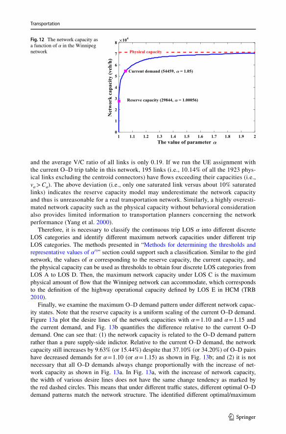
Without loss of generality, Fig.  11 depicts the convergence curve of the solution algorithm at α = 1.5. The CPU time for α = 1.5 is 4454 s. Note that the tolerance error of the relative gap is set at 1E-6, which is much stricter than the typical value of 1E-4 suggested by Boyce et al. (2004). If the tolerance error is set at 1E-4, the CPU time for α = 1.5 will be 812 s, i.e., 18.24% of 4454 s. The above results verify the efficiency of the solution algorithm in solving the proposed model in large-scale networks. Then, we examine the effect of the O–D-based LOS requirement (i.e., different values of α) on the resultant maximum capacity in the Winnipeg network as shown in Fig. 12. Consist-ent with the grid network, the proposed α-max capacity offers great flexibility to model

Table 5 The results of link volumes and maximum O–D demands from the proposed models with hard con-straints and soft constraints (α = 1.5)

Error =|hard-soft|/hard × 100%

Link Volume (veh/min) Maximum O–D Demand (veh/min)

Link Hard Soft Error Link Hard Soft Error O–D Hard Soft Error

1 99.60 101.27 1.67% 10 478.00 476.42 0.33% (1, 6) 240 240.00 0.00%2 286.40 285.29 0.39% 11 250.00 248.41 0.64% (1, 8) 226 225.29 0.31%3 280.00 278.74 0.45% 12 0.00 0.00 NA (1, 9) 200 200.00 0.00%4 255.60 256.43 0.33% 13 350.00 349.78 0.06% (2, 6) 194 192.56 0.74%5 600.00 599.44 0.09% 14 220.00 218.85 0.52% (2, 8) 382 382.05 0.01%6 255.60 256.43 0.33% (2, 9) 180 180.00 0.00%7 186.40 182.77 1.95% (4, 6) 160 160.00 0.00%8 350.00 349.78 0.06% (4, 8) 0 0 NA9 338.40 336.13 0.67% (4, 9) 90 87.26 3.04%

Transportation

1 3

the Winnipeg network capacity in a broad range from 0 to 72,531 (veh/h) (i.e., physi-cal capacity), including the reserve capacity (29,844 veh/h) and the current demand (54,459 veh/h) as special cases of our proposed model despite that their corresponding LOS requirements are not known a prior. In fact, the corresponding values of α for the reserve capacity and current demand are 1.00056 and 1.050, respectively. There is a large gap between the reserve capacity and the current demand (24,615 veh/h) as well as the gap between the reserve capacity and the physical capacity (42,687 veh/h). Besides, in the reserve capacity model, only one link reaches its capacity constraint

Fig. 10 Winnipeg network

Fig. 11 The convergence curve of the solution algorithm (α = 1.5)

0 1000 2000 3000 4000 500010

-6

10-5

10-4

10-3

10-2

10-1

100

CPU time (s)

Rel

ativ

e ga

p

812s

Transportation

1 3

and the average V/C ratio of all links is only 0.19. If we run the UE assignment with the current O–D trip table in this network, 195 links (i.e., 10.14% of all the 1923 phys-ical links excluding the centroid connectors) have flows exceeding their capacities (i.e., va > Ca). The above deviation (i.e., only one saturated link versus about 10% saturated links) indicates the reserve capacity model may underestimate the network capacity and thus is unreasonable for a real transportation network. Similarly, a highly overesti-mated network capacity such as the physical capacity without behavioral consideration also provides limited information to transportation planners concerning the network performance (Yang et al. 2000).

Therefore, it is necessary to classify the continuous trip LOS α into different discrete LOS categories and identify different maximum network capacities under different trip LOS categories. The methods presented in “Methods for determining the thresholds and representative values of αrs” section could support such a classification. Similar to the gird network, the values of α corresponding to the reserve capacity, the current capacity, and the physical capacity can be used as thresholds to obtain four discrete LOS categories from LOS A to LOS D. Then, the maximum network capacity under LOS C is the maximum physical amount of flow that the Winnipeg network can accommodate, which corresponds to the definition of the highway operational capacity defined by LOS E in HCM (TRB 2010).

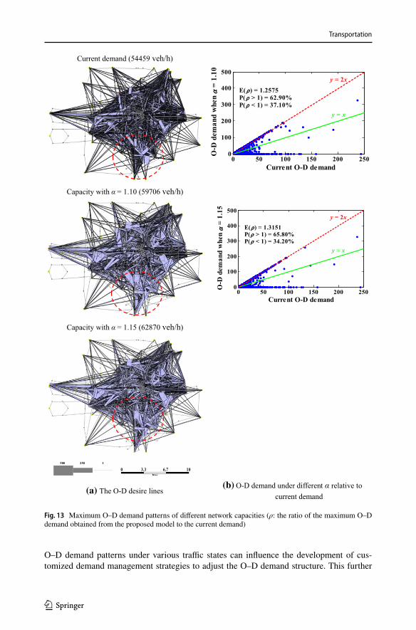
Finally, we examine the maximum O–D demand pattern under different network capac-ity states. Note that the reserve capacity is a uniform scaling of the current O–D demand. Figure 13a plot the desire lines of the network capacities with α = 1.10 and α = 1.15 and the current demand, and Fig.  13b quantifies the difference relative to the current O–D demand. One can see that: (1) the network capacity is related to the O–D demand pattern rather than a pure supply-side indictor. Relative to the current O–D demand, the network capacity still increases by 9.63% (or 15.44%) despite that 37.10% (or 34.20%) of O–D pairs have decreased demands for α = 1.10 (or α = 1.15) as shown in Fig. 13b; and (2) it is not necessary that all O–D demands always change proportionally with the increase of net-work capacity as shown in Fig.  13a. In Fig.  13a, with the increase of network capacity, the width of various desire lines does not have the same change tendency as marked by the red dashed circles. This means that under different traffic states, different optimal O–D demand patterns match the network structure. The identified different optimal/maximum

Fig. 12 The network capacity as a function of α in the Winnipeg network

Transportation

1 3

O–D demand patterns under various traffic states can influence the development of cus-tomized demand management strategies to adjust the O–D demand structure. This further

Current demand (54459 veh/h)

Capacity with = 1.10 (59706 veh/h)

Capacity with = 1.15 (62870 veh/h)

500 250 1

0 3.3 6.7 10

(a) The O-D desire lines(b) O-D demand under different relative to

current demand

0 50 100 150 200 2500

100

200

300

400

500

Current O-D demand

O-D

dem

and

whe

n αα

= 1

.10

E(ρρ) = 1.2575P(ρρ > 1) = 62.90%P(ρρ < 1) = 37.10%

y = 2x

y = x

0 50 100 150 200 2500

100

200

300

400

500

Current O-D demand

O-D

dem

and

whe

n αα

= 1

.15

E(ρρ) = 1.3151P(ρρ > 1) = 65.80%P(ρρ < 1) = 34.20%

y = 2x

y = x

Fig. 13 Maximum O–D demand patterns of different network capacities (ρ: the ratio of the maximum O–D demand obtained from the proposed model to the current demand)

Transportation

1 3

verifies that the proposed model can support traffic managers to adopt flexible management and control measures according to traffic states.

Concluding remarks

In this paper, we proposed the α-max network capacity model with the O–D-based LOS requirement to surmount the disadvantages associated with the existing MP-based network capacity models, i.e., the inconsideration of LOS in single-level MP and non-convexity of BLP. Mathematically, the α-max network capacity model was formulated as a single-level MP using the excess-demand network augmentation. Specifically, the virtual path cost for each O–D pair in the augmented network was determined by trip LOS requirement, which makes the proposed model flexible to estimate the network capacity under various traffic conditions. For practical use, we further provided methods to convert continuous trip LOS into discrete trip LOS categories and to obtain the network capacity under representative traffic states. This classification is useful in supporting the development of active manage-ment measures, such as setting the maximum trip cost as the desired value to control the network capacity for special purposes. A modified gradient projection algorithm with soft constraint technique was developed to solve the proposed method. Two networks were used to examine the features of the proposed model and the efficiency of the solution algorithm.

In summary, the computational and behavioral advantages of the proposed α-max capacity model compared to the existing network capacity models are as follows:

• It consider the trip LOS requirement, which offers flexibility to estimate the network capacity from zero to physical capacity. The existing reserve capacity and ultimate capacity models can be viewed as special cases of the proposed model despite that their corresponding LOS requirements are not known a prior. This flexibility also makes it possible to identify different critical or saturated links according to different traffic states, which is useful to support meticulous management and control.

• The consideration of O–D-based (i.e., trip) LOS has two benefits compared with the link-based LOS. Firstly, the O–D-based LOS requirement can intuitively reflect the maximum travel cost, which is the price that travelers are willing to pay for a travel and thus more important than the operating conditions of a single link (i.e., the link-based LOS) for travelers. Secondly, planners and managers usually pay more attention to the O–D travel time and even directly set certain O–D travel time as one of their planning targets. Consequently, the consideration of O–D-based LOS in the proposed model can help planners and managers know how many traffic flows the transportation network can accommodate under a certain requirement of O–D-based LOS. The result is a key information for planners and managers to take flexible and effective measures for guar-anteeing their planning targets.

• It is convex and single-level MP, which is convenient for developing a computationally efficient solution algorithm for large-scale network applications. This has been verified in the Winnipeg network.

For future research, several directions are worthy of further investigations. It is interest-ing to integrate the concept of reserve capacity into the proposed model. In other words, we can use the current O–D cost to replace the shortest free-flow path cost τmin in the virtual path cost for each O–D pair, which means that we preserve the fixed O–D cost pattern just

Transportation

1 3

like the fixed O–D demand pattern preserved in the reserve capacity model. Also, we plan to extend the proposed model to a multi-modal transportation network with both physical capacity constraints and environmental constraints (Chen et  al. 2011b). Besides, we can explore various applications of the proposed model, such as car ownership estimation, net-work design, environmental capacity estimation, etc. At last, since the MP-based approach and the MFD approach are two different approaches for estimating the network capacity, it is interesting and important to collect consistent data for these two approaches and then investigate their relationship (particularly whether there are analytical linkages) in future studies.

Authors’ contributions All authors contributed to the study conception and design. Material preparation, data collection and analysis were performed by Zhaoqi Zang, and Xiangdong Xu. The first draft of the manuscript was written by Zhaoqi Zang, and all authors commented on previous versions of the manuscript. All authors read and approved the final manuscript.

Funding This study is supported by the National Key Research and Development Program of China (No. 2018YFB1600900), National Natural Science Foundation of China (71971159, U1764261, and 71890973), the Shanghai Rising-Star Program (20QA1409800), and the Research Grants Council of the Hong Kong Special Administrative Region (15212217). These supports are gratefully acknowledged.

Availability of data and material Open dataset available at https:// github. com/ bstab ler/ Trans porta tionN etwor ks.

Code availability Code is available on request.

Declarations

Conflict of interest On behalf of all authors, the corresponding author states that there is no conflict of inter-est.

Open Access This article is licensed under a Creative Commons Attribution 4.0 International License, which permits use, sharing, adaptation, distribution and reproduction in any medium or format, as long as you give appropriate credit to the original author(s) and the source, provide a link to the Creative Com-mons licence, and indicate if changes were made. The images or other third party material in this article are included in the article’s Creative Commons licence, unless indicated otherwise in a credit line to the material. If material is not included in the article’s Creative Commons licence and your intended use is not permitted by statutory regulation or exceeds the permitted use, you will need to obtain permission directly from the copyright holder. To view a copy of this licence, visit http:// creat iveco mmons. org/ licen ses/ by/4. 0/.

References

Akamatsu, T., Miyawaki, O.: Maximum network capacity problem under the transportation equilibrium assignment (in Japanese). Infrastruct. Plan. Rev. 12, 719–729 (1995)

Akamatsu, T., Wada, K.: Tradable network permits: A new scheme for the most efficient use of network capacity. Transp. Res. Part C 79, 178–195 (2017)

Asakura Y (1992) Maximum capacity of road network constrained by user equilibrium conditions. Paper presented at the 24th Annual UTSG Conference, UK.

Asakura, Y., Kashiwadani, M.: Estimation model of maximum road network capacity with parking con-straints and its application (in Japanese). Infrastruct. Plan. Rev. 11, 129–136 (1993)

Beckmann, M., McGuire, C.B., Winsten, C.B.: Studies in the Economics of Transportation. Yale University Press, New Haven (1956)

Bell, M.G., Kurauchi, F., Perera, S., Wong, W.: Investigating transport network vulnerability by capacity weighted spectral analysis. Transp. Res. Part B 99, 251–266 (2017)

Transportation

1 3

Boyacı, B., Geroliminis, N.: Estimation of the network capacity for multimodal urban systems. Procedia Soc. Behav. Sci. 16, 803–813 (2011)

Boyce, D., Ralevic-Dekic, B., Bar-Gera, H.: Convergence of traffic assignments: How much is enough? J. Transp. Eng. 130(1), 49–55 (2004)

Ceylan, H., Bell, M.G.: Reserve capacity for a road network under optimized fixed time traffic signal con-trol. J. Intell. Transp. Syst. 8(2), 87–99 (2004)

Chen, A., Kasikitwiwat, P.: Modeling network capacity flexibility of transportation networks. Transp. Res. Part A 45(2), 105–117 (2011)

Chen, A., Kasikitwiwat, P., Yang, C.: Alternate capacity reliability measures for transportation networks. J. Adv. Transp. 47(1), 79–104 (2013)

Chen, A., Yang, H., Lo, H.K., Tang, W.H.: Capacity reliability of a road network: an assessment methodol-ogy and numerical results. Transp. Res. Part B 36(3), 225–252 (2002)

Chen, A., Zhou, Z., Chootinan, P., Ryu, S., Yang, C., Wong, S.C.: Transport network design problem under uncertainty: A review and new developments. Transp. Rev. 31(6), 743–768 (2011a)

Chen, A., Zhou, Z., Ryu, S.: Modeling physical and environmental side constraints in traffic equilibrium problem. Int. J. Sustain. Transp. 5, 172–197 (2011b)

Cheng, Z., Wang, W., Lu, J., Xing, X.: Classifying the traffic state of urban expressways: a machine-learning approach. Transp. Res. Part A 137, 411–428 (2020)

Chinazzi, M., Davis, J.T., Ajelli, M., Gioannini, C., Litvinova, M., Merler, S., Piontti, A.P., Mu, K., Rossi, L., Sun, K., Viboud, C.: The effect of travel restrictions on the spread of the 2019 novel coronavirus (COVID-19) outbreak. Science 368(6489), 395–400 (2020)

Chiou, S.: Optimal signal-setting for road network with maximum capacity. Inf. Sci. 273, 287–303 (2014)

Farvaresh, H., Sepehri, M.M.: A branch and bound algorithm for bi-level discrete network design prob-lem. Netw. Spat. Econ. 13(1), 67–106 (2013)

Feng, L., Xie, J., Nie, Y., Liu, X.: Efficient algorithm for the traffic assignment problem with side con-straints. Transp. Res. Rec. 2674(4), 129–139 (2020)

Gao, Z.Y., Song, Y.F.: A reserve capacity model of optimal signal control with user-equilibrium path choice. Transp. Res. Part B 36(4), 313–323 (2002)

Geroliminis, N., Boyacı, B.: The effect of variability of urban systems characteristics in the network capacity. Transp. Res. Part B 46(10), 1607–1623 (2012)

Iida, Y.: Methodology for maximum capacity of road network. Trans. Jpn. Soc. Civ. Eng. 205, 147–150 (1972)

Inouye, H., 1987. Traffic equilibria and its solution in congested road networks. In: Genser, R. (Ed.), Proceedings of IFAC Conference on Control in Transportation Systems, 267–272.

INRO Consultants., 1999. Emme/2 user’s manual. Montréal, CanadaKarin, O., Bar-On, Y., Milo, T., Katzir, I., Mayo, A., Korem, Y., Dudovich, B., Zehavi, A., Davidovich,

N., Milo, R., Alon, U., 2020. Adaptive cyclic exit strategies from lockdown to suppress COVID-19 and allow economic activity. medRxiv . https:// doi. org/ 10. 1101/ 2020. 04. 04. 20053 579.

Koh, A., Shepherd, S., Sumalee, A.: Second best toll and capacity optimisation in networks: solution algorithm and policy implications. Transportation 36, 147–165 (2009)

Larsson, T., Patriksson, M.: An augmented Lagrangian dual algorithm link capacity side constrained traffic assignment problems. Transp. Res. 29B, 433–455 (1995)

Lau, H., Khosrawipour, V., Kocbach, P., Mikolajczyk, A., Schubert, J., Bania, J., Khosrawipour, T.: The positive impact of lockdown in Wuhan on containing the COVID-19 outbreak in China. J. Travel Med. 27(3), 1–7 (2020)

Lo, H.K., Tung, Y.K.: Network with degradable links: Capacity analysis and design. Transp. Res. Part B 37(4), 345–363 (2003)

Luathep, P., Sumalee, A., Lam, W.H., Li, Z.C., Lo, H.K.: Global optimization method for mixed trans-portation network design problem: a mixed-integer linear programming approach. Transp. Res. Part B 45(5), 808–827 (2011)

Mazloumian, A., Geroliminis, N., Helbing, D.: The spatial variability of vehicle densities as determinant of urban network capacity. Philos. Trans. R. Soc. Math. Phys. Eng. Sci. 368(1928), 4627–4647 (2010)

Miandoabchi, E., Farahani, R.Z.: Optimizing reserve capacity of urban road networks in a discrete net-work design problem. Adv. Eng. Softw. 42(12), 1041–1050 (2011)

New York: One New York: The Plan for a Strong and Just City, New York, USA (2015).Nguyen, S., Pallottino, S., Malucelli, F.: A modeling framework for passenger assignment on a transport

network with timetables. Transp. Sci. 35, 238–249 (2001)Nie, Y., Zhang, H.M., Lee, D.-H.: Models and algorithms for the traffic assignment problem with link

capacity constraints. Transp. Res. Part B 38, 285–312 (2004)

Transportation

1 3

Noh, H.: Capacitated schedule-based transit assignment using a capacity penalty cost. Ph.D. Disserta-tion. The University of Arizona, Arizona, USA (2013).

Patriksson, M.: Algorithms for computing traffic equilibria. Netw. Spat. Econ. 4(1), 23–38 (2004)Patriksson, M.: The Traffic Assignment Problem: Models and Methods. Courier Dover Publications,

New York (2015)Possel, B., Wismans, L.J.J., Berkum, E.C.V., Bliemer, M.C.J.: The multi-objective network design prob-

lem using minimizing externalities as objectives: comparison of a genetic algorithm and simulated annealing framework. Transportation 45(2), 1–28 (2018)

Ryu, S., Chen, A., Choi, K.: A modified gradient projection algorithm for solving the elastic demand traffic assignment problem. Comput. Oper. Res. 47, 61–71 (2014a)

Ryu, S., Chen, A., Xu, X.,: Application of gradient projection algorithm for solving the user equilibrium traffic assignment problem with soft link capacity constraints. Transportation Research Board 96th Annual Meeting, Washington D.C. (2017)

Ryu, S., Chen, A., Xu, X., Choi, K.: A dual approach for solving the combined distribution and assignment problem with link capacity constraints. Netw. Spat. Econ. 14(2), 245–270 (2014b)

Saberi, M., Mahmassani, H.S., Zockaie, A.: Network capacity, traffic instability, and adaptive driving: find-ings from simulated urban network experiments. EURO J. Transp. Logist. 3(3), 289–308 (2015)

Shanghai: Shanghai city overall plan (2017–2035): Striving for the Excellent Global City, Shanghai, China (2017).

Sheffi, Y.: Urban Transportation Networks: Equilibrium Analysis with Mathematical Programming Meth-ods. Prentice-Hall, NJ (1985)

Shi, F., Xu, G.M., Huang, H.: An augmented Lagrangian origin-based algorithm for link-capacitated traffic assignment problem. J. Adv. Transp. 49(4), 553–567 (2015)

Tam, M.L., Lam, W.H.: Maximum car ownership under constraints of road capacity and parking space. Transp. Res. Part A 34(3), 145–170 (2000)

TRB:. Highway Capacity Manual 2000. Transportation Research Board, National Research Council, Wash-ington DC, USA (2000)

TRB: Highway Capacity Manual 2010. Transportation Research Board, National Research Council, Wash-ington DC, USA (2010)

Wang, D.Z.W., Lo, H.: Global optimum of the linearized network design problem with equilibrium flows. Transp. Res. Part B 44, 482–492 (2010)

Wang, J., Du, M., Lu, L., He, X.: Maximizing network throughput under stochastic user equilibrium with elastic demand. Netw. Spat. Econ. 18(1), 115–143 (2018)

Wang, J., Wang, H., Zhang, X.: A hybrid management scheme with parking pricing and parking permit for a many-to-one park and ride network. Transp. Res. Part C 112, 153–179 (2020)

Wong, S.C., Yang, H.: Reserve capacity of a signal-controlled road network. Transp. Res. Part B 31(5), 397–402 (1997)

Xu, M., Wang, G., Grant-Muller, S., Gao, Z.: Joint road toll pricing and capacity development in discrete transport network design problem. Transportation 44(4), 731–752 (2017)

Xu, X., Chen, A., Yang, C.: An optimization approach for deriving upper and lower bounds of transporta-tion network vulnerability under simultaneous disruptions of multiple links. Transp. Res. Part C 94, 338–353 (2018a)

Xu, X., Chen, A., Jansuwan, S., Yang, C., Ryu, S.: Transportation network redundancy: Complementary measures and computational methods. Transp. Res. Part B 114, 68–85 (2018b)

Yan, F.: Urban public transportation demand prediction and ridesharing optimization based on multisource data (in Chinese). Ph.D. Dissertation. Tongji University, Shanghai, China (2019)

Yang, H., Bell, M.G.H.: Models and algorithms for road network design: a review and some new develop-ments. Transp. Rev. 18(3), 257–278 (1998)

Yang, H., Bell, M.G.H., Meng, Q.: Modeling the capacity and level of service of urban transportation net-works. Transp. Res. Part B 34(4), 255–275 (2000)

Yang, H., Huang, H.J.: Mathematical and Economic Theory of Road Pricing. Elsevier, New York (2005)Yang, H., Yagar, S.: Traffic assignment and traffic control in general freeway-arterial corridor system.

Transp. Res. 28B, 463–486 (1994)Yang, H., Yagar, S.: Traffic assignment and signal control in saturated road networks. Transp. Res. 29A,

125–139 (1995)Yildirimoglu, M., Geroliminis, N.: Approximating dynamic equilibrium conditions with macroscopic fun-

damental diagrams. Transp. Res. Part B 70, 186–200 (2014)Yim, K., Wong, S.C., Chen, A., Wong, C.K., Lam, W.H.K.: A reliability-based land use and transportation

optimization model. Transp. Res. Part C 19(2), 351–362 (2011)Zhang, P., Qian, Z.S.: Managing traffic with raffles. Transp. Res. Part C 107, 490–509 (2019)

Transportation

1 3

Zhang, Y., Zhang, A., Wang, J.: Exploring the roles of high-speed train, air and coach services in the spread of COVID-19 in China. Transp. Policy 94, 34–42 (2020)

Publisher’s Note Springer Nature remains neutral with regard to jurisdictional claims in published maps and institutional affiliations.

Zhaoqi Zang will be a Ph.D. student in the School of Civil and Environmental Engineering at the Nan-yang Technological University. He obtained his bachelor’s and master’s degrees from Tongji University. His research interests include travel time reliability and its valuation, and network modeling and optimization.

Xiangdong Xu is a professor in the College of Transportation Engineering at Tongji University. His research interests include transportation network modeling and optimization, transportation systems resiliency analy-sis, network flow estimation and sensors location, and integration of model-driven and data-driven transpor-tation systems analytics.

Anthony Chen is a professor of the Department of Civil and Environmental Engineering at The Hong Kong Polytechnic University. His research interests include transportation systems modeling and analysis, trans-portation network reliability/vulnerability/flexibility/redundancy/resiliency analysis, transportation network design under uncertainty, path flow estimator and its applications in transportation planning, and applied optimization to civil infrastructure problems.

Chao Yang is a professor in the College of Transportation Engineering at Tongji University. His research interests include traffic big data analysis, transportation network modeling and analysis, traffic planning technology, and traffic demand forecasting.

Authors and Affiliations

Zhaoqi Zang1 · Xiangdong Xu1  · Anthony Chen2 · Chao Yang1

Zhaoqi Zang zangzhaoqi@126.com

Anthony Chen anthony.chen@polyu.edu.hk

Chao Yang tongjiyc@tongji.edu.cn

1 Key Laboratory of Road and Traffic Engineering of the Ministry of Education, Tongji University, Shanghai, China

2 Department of Civil and Environmental Engineering, The Hong Kong Polytechnic University, Kowloon, Hong Kong, China