Modeling a Carrington-scale Stellar Superflare and Coronal Mass Ejection from k Cet1

Benjamin J. Lynch1 , Vladimir S. Airapetian2,3 , C. Richard DeVore2 , Maria D. Kazachenko4 , Teresa Lüftinger5,Oleg Kochukhov6 , Lisa Rosén6, and William P. Abbett1

1 Space Sciences Laboratory, University of California–Berkeley, Berkeley, CA 94720, USA; blynch@ssl.berkeley.edu2 NASA Goddard Space Flight Center, Greenbelt, MD 20771, USA

3 Department of Physics, American University, Washington, D.C. 20016, USA4 Laboratory for Atmospheric and Space Physics, University of Colorado, Boulder, CO 80303, USA

5 Department of Astrophysics, University of Vienna, Vienna, Austria6 Department of Physics and Astronomy, Uppsala University, Uppsala, Sweden

Received 2019 April 9; revised 2019 June 3; accepted 2019 June 7; published 2019 July 30

Abstract

Observations from the Kepler mission have revealed frequent superflares on young and active solar-like stars.Superflares result from the large-scale restructuring of stellar magnetic fields, and are associated with the eruptionof coronal material (a coronal mass ejection, or CME) and energy release that can be orders of magnitude greaterthan those observed in the largest solar flares. These catastrophic events, if frequent, can significantly impact thepotential habitability of terrestrial exoplanets through atmospheric erosion or intense radiation exposure at thesurface. We present results from numerical modeling designed to understand how an eruptive superflare from ayoung solar-type star, κ1Cet, could occur and would impact its astrospheric environment. Our data-inspired, three-dimensional magnetohydrodynamic modeling shows that global-scale shear concentrated near the radial-fieldpolarity inversion line can energize the closed-field stellar corona sufficiently to power a global, eruptive superflarethat releases approximately the same energy as the extreme 1859 Carrington event from the Sun. We examineproxy measures of synthetic emission during the flare and estimate the observational signatures of our CME-drivenshock, both of which could have extreme space-weather impacts on the habitability of any Earth-like exoplanets.We also speculate that the observed 1986 Robinson-Bopp superflare from κ1Cet was perhaps as extreme for thatstar as the Carrington flare was for the Sun.

Key words: magnetohydrodynamics (MHD) – solar–terrestrial relations – stars: magnetic field – stars: solar-type –Sun: coronal mass ejections (CMEs) – Sun: flares

Supporting material: animations

1. Introduction

There is growing appreciation that planetary atmosphericchemistry, and even the retention of an atmosphere in manycases, depends critically upon the high-energy radiation andparticle environments around the host star (Segura et al. 2005;Cohen et al. 2014; Domagal-Goldman et al. 2014; Rugheimeret al. 2015). This has led to a number of increasinglysophisticated modeling efforts to characterize the spaceenvironment of exoplanets and stellar-wind/exoplanet interac-tions (Cohen et al. 2011; Vidotto et al. 2011, 2012; Garraffoet al. 2016, 2017; Garcia-Sage et al. 2017). The cumulativeeffects of both steady-state and extreme space weather fromactive stars, including intense X-ray and extreme ultraviolet(EUV) radiation, large fluxes of highly energetic particles, andfrequent exoplanet interactions with stellar coronal massejections (CMEs), will have a significant impact on theexoplanets’ atmospheric evolution, and ultimately on theirhabitability (Lammer et al. 2007, 2009; Drake et al. 2013;Osten & Wolk 2015; Kay et al. 2016; Airapetian et al. 2019a).Additionally, stellar activity from young solar-type stars, suchas κ1Cet, is now being considered in investigations of theevolution of our own solar system, where enhanced levels ofextreme space weather may have profoundly affected thechemistry and climate of the early Earth (Airapetian et al.2016b, 2017; Dong et al. 2017; Garcia-Sage et al. 2017).

Solar flares—the explosive release of energy in the solaratmosphere across a wide range of electromagnetic wave-lengths—occur due to the rapid release of free energy stored in

the strong sheared and/or twisted magnetic fields typicallyassociated with sunspots and active regions (Forbes 2000;Fletcher et al. 2011; Kazachenko et al. 2012). Solar flares andCMEs are widely, although not universally, accepted as beingdriven by magnetic reconnection (Klimchuk 2001; Lynch et al.2008; Karpen et al. 2012). The long-standing CSHKP model(Carmichael 1964; Sturrock 1966; Hirayama 1974; Kopp &Pneuman 1976) for eruptive solar flares explains many of theirgeneric observed properties (e.g., Janvier et al. 2015; Lynchet al. 2016; Welsch 2018, and references therein).The total energy released during solar flares typically ranges

over E∼1029–32 erg (Emslie et al. 2012), whereas stellar flarescan extend to a much higher range of energies E∼1032–36 erg(Shibata et al. 2013; Maehara et al. 2015; Notsu et al. 2019).Kepler observations of superflaring solar-type stars indicatethat large starspots typically are associated with their flares, thefrequency and maximum energy of the flares depend criticallyupon the age of the star, and younger stars exhibit greatermaximum flare energies and higher flare frequencies (Maeharaet al. 2012; Notsu et al. 2013, 2019; Shibayama et al. 2013).Schaefer et al. (2000) presented some of the earliest

superflare observations associated with solar-type stars,including κ1Cet, a G5 young solar analog aged ∼0.7Gyr.They estimated the κ1Cet superflare energy asE∼2×1034 erg, based on observations by Robinson &Bopp (1987) of He I emission. κ1Cet is reported as havingmagnetic cycles and magnetic field strengths in the kiloGaussrange (Saar & Baliunas 1992) and showing evidence of

The Astrophysical Journal, 880:97 (12pp), 2019 August 1 https://doi.org/10.3847/1538-4357/ab287e© 2019. The American Astronomical Society. All rights reserved.

1

starspots that rotate differentially across the stellar disk(Rucinski et al. 2004; Walker et al. 2007). The star’s quasi-steady wind and radiation environments are objects of ongoingstudy for their effects on planetary habitability (e.g., Ribas et al.2010; do Nascimento et al. 2016).In this paper, we present results from a three-dimensional

numerical magnetohydrodynamics (MHD) simulation of aglobal stellar superflare and its CME, based on observations byRosén et al. (2016) of the magnetic field of κ1Cet. Althoughstellar active-region fields associated with large starspots arethought to contain the magnetic free energy necessary to powersuperflares and their associated eruptions, stellar magnetogramobservations tend to leave such strong-field regions unresolved.Our approach is to model self-consistently the gradualaccumulation of free magnetic energy via the introduction oflarge-scale stresses to the observed global stellar field. In thisway, we maximize both the amount of free energy available forrelease during the eruptive flare and the spatial scale of thestellar CME, without making any assumptions about theexistence or strength of unresolved starspots on κ1Cet.Therefore, our global-scale eruption represents the mostextreme stellar space-weather event possible within theobserved constraints on the surface magnetic flux distribution,and sets a baseline for comparison with observations ofsuperflares on κ1Cet and similar stars.

Our paper is organized as follows. In Section 2 we presentthe MHD numerical model. Section 3 describes the pre-eruption phase of the simulation, including the magnetic fieldconfiguration (Section 3.1), the stellar-wind outflow(Section 3.2), and the self-consistent, slowly driven energy-accumulation phase (Section 3.3). In Section 4 we present theeruption results and their analysis: the global-eruption over-view and energy evolution (Section 4.1), the stellar-flarereconnected flux (Section 4.2), the synthetic X-ray and EUVemission proxies (Section 4.3), and the properties of the CME-driven shock (Section 4.4). Section 5 concludes with adiscussion of our results in the context of future modelingand observations of stellar space weather.

2. Adaptively Refined MHD Solver (ARMS)

The ARMS code, developed by DeVore & Antiochos (2008)and collaborators, calculates solutions to the 3D nonlinear,time-dependent MHD equations that describe the evolution andtransport of density, momentum, energy, and magnetic fluxthroughout the system. The numerical scheme used is a finite-volume, multidimensional flux-corrected transport algorithm(DeVore 1991). ARMS is fully integrated with the adaptive-mesh toolkit PARAMESH (MacNeice et al. 2000) to handledynamic, solution-adaptive grid refinement and enable efficientmultiprocessor parallelization. For our simulation, we useARMS to solve the following ideal MHD equations inspherical coordinates

rr

¶¶

+ =Vt

0, 1· ( ) ( )

r rp

r¶¶

+ + = ´ ´ -V VV B B gt

P1

4, 2( ) · ( ) ( ) ( )

¶¶

= ´ ´B

V Bt

, 3( ) ( )

where all the variables retain their usual meaning, solar gravityis = -g rg r R 2( ) ˆ with ge=2.75×104 cms−2, and we

use the ideal gas law r=P m k T2 p B( ) . Given the isothermalapproximation used in the construction of our background solarwind, we do not solve an internal energy or temperatureequation. The plasma temperature remains uniform throughoutthe domain for the duration of the simulation.Additionally, while there is no explicit magnetic resistivity in

the equations of ideal MHD, necessary, and stabilizingnumerical diffusion terms introduce an effective resistivity onvery small spatial scales, i.e., the size of the grid. In this way,magnetic reconnection can occur when current sheet featuresand the associated gradients of field reversals have beendistorted and compressed to the local grid scale.The spherical computational domain uses logarithmic grid

spacing in r and uniform grid spacing in θ, f. The domainextends from Îr R R1 , 30[ ] , θä[11°.25, 168°.75] (±78°.75in latitude), and fä[−180°, +180°] (longitude). The initialgrid consists of 6×6×12 blocks with 83 grid cells per block.There are two additional levels of static grid refinement. Thehighest refinement region (level 3) is Îr R R1 , 5.485[ ] forall θ, f, and the level 2 refinement extends fromÎr R R5.485 , 9.650[ ] . The maximum resolution is there-

fore 192×192×384, with the level 3 grid cells having anangular width of 0°.820×0°.938 in θ, f and a radial extent ofΔr=0.01787 Re at the lower boundary. After the solar windrelaxation phase we turn on the adaptive-mesh refinementcriteria. The maximum refinement remains at level 3 but as theeruption progresses and regions of high electric current densityevolve, the computational grid refines and de-refines to trackthe evolution of the strong currents. The refinement criteria aredescribed in Karpen et al. (2012).

3. Pre-eruption Stellar Corona

3.1. Magnetic Field Configuration

For decades, the fossil magnetic fields of massive, early-typestars were analyzed assuming simple dipole or dipole-plus-quadrupole magnetic field geometries. For late-type activestars, the development of Zeeman-Doppler imaging (ZDI;Donati & Brown 1997; Piskunov & Kochukhov 2002) hasmade it possible to invert time series of high-resolutionspectroscopic and spectropolarimetric Stokes observations(circularly and linearly polarized stellar light) into surfacemaps of parameters such as brightness, temperature, elementalabundance, and complex magnetic field geometry (Lüftingeret al. 2010a, 2010b). ZDI has further matured and can now beused to determine the strength, distribution, polarity, andpolarity reversals of surface magnetic fields (Lüftinger et al.2015; Kochukhov 2016). The availability of stellar magneticfield maps has significantly advanced our capacity forsophisticated numerical modeling of stellar coronae, winds,and star–planet interactions (Cohen et al. 2011; Vidotto et al.2011; do Nascimento et al. 2016; Garraffo et al. 2016).In our numerical simulation, we use the κ1Cet surface field

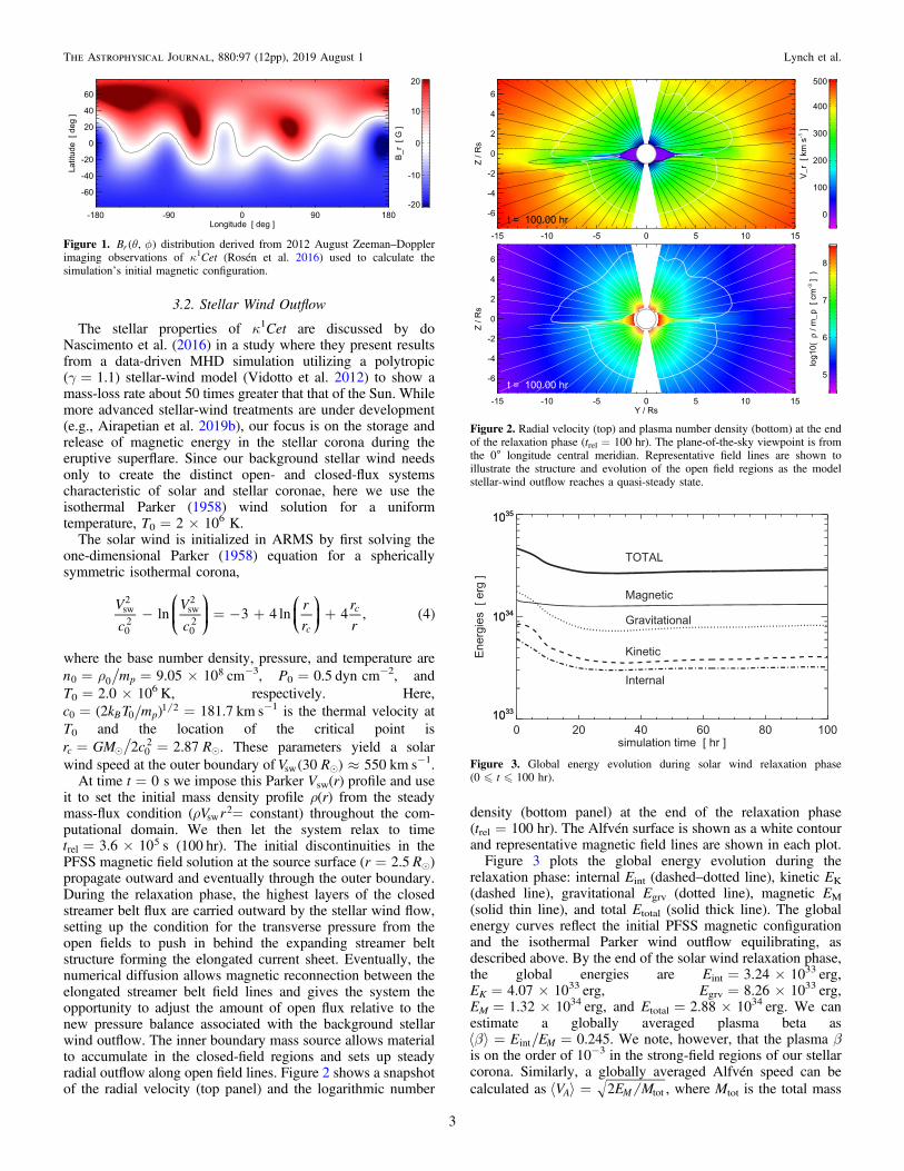
distribution from Rosén et al. (2016) during the epoch 2012.9(mid-to-late August) derived from the ZDI analysis of datafrom PolarBase (Petit et al. 2014). Figure 1 shows this q fB ,r ( )distribution at the lower radial boundary. A positive radial fieldis denoted as red, a negative radial field is blue, and the blackline indicates the Br=0 polarity inversion line (PIL). Wegenerate the potential field source surface (PFSS; Wang &Sheeley 1992) solution, which is used to initialize the magneticfield throughout the computational domain.

2

The Astrophysical Journal, 880:97 (12pp), 2019 August 1 Lynch et al.

3.2. Stellar Wind Outflow

The stellar properties of κ1Cet are discussed by doNascimento et al. (2016) in a study where they present resultsfrom a data-driven MHD simulation utilizing a polytropic(γ=1.1) stellar-wind model (Vidotto et al. 2012) to show amass-loss rate about 50 times greater that that of the Sun. Whilemore advanced stellar-wind treatments are under development(e.g., Airapetian et al. 2019b), our focus is on the storage andrelease of magnetic energy in the stellar corona during theeruptive superflare. Since our background stellar wind needsonly to create the distinct open- and closed-flux systemscharacteristic of solar and stellar coronae, here we use theisothermal Parker (1958) wind solution for a uniformtemperature, T0=2×106 K.

The solar wind is initialized in ARMS by first solving theone-dimensional Parker (1958) equation for a sphericallysymmetric isothermal corona,

- = - + +V

c

V

c

r

r

r

rln 3 4 ln 4 , 4

c

csw2

02

sw2

02

⎛⎝⎜

⎞⎠⎟

⎛⎝⎜

⎞⎠⎟ ( )

where the base number density, pressure, and temperature arer= = ´n m 9.05 10p0 0

8 cm−3, P0=0.5 dyncm−2, andT0=2.0×106 K, respectively. Here,

= =c k T m2 181.7B p0 01 2( ) km s−1 is the thermal velocity at

T0 and the location of the critical point is= =r GM c R2 2.87c 0

2 . These parameters yield a solar

wind speed at the outer boundary of »V R30 550sw( ) km s−1.At time t=0s we impose this Parker Vsw(r) profile and use

it to set the initial mass density profile ρ(r) from the steadymass-flux condition (r =V rsw

2 constant) throughout the com-putational domain. We then let the system relax to time

= ´t 3.6 10 srel5 (100 hr). The initial discontinuities in the

PFSS magnetic field solution at the source surface (r=2.5 Re)propagate outward and eventually through the outer boundary.During the relaxation phase, the highest layers of the closedstreamer belt flux are carried outward by the stellar wind flow,setting up the condition for the transverse pressure from theopen fields to push in behind the expanding streamer beltstructure forming the elongated current sheet. Eventually, thenumerical diffusion allows magnetic reconnection between theelongated streamer belt field lines and gives the system theopportunity to adjust the amount of open flux relative to thenew pressure balance associated with the background stellarwind outflow. The inner boundary mass source allows materialto accumulate in the closed-field regions and sets up steadyradial outflow along open field lines. Figure 2 shows a snapshotof the radial velocity (top panel) and the logarithmic number

density (bottom panel) at the end of the relaxation phase(trel=100 hr). The Alfvén surface is shown as a white contourand representative magnetic field lines are shown in each plot.Figure 3 plots the global energy evolution during the

relaxation phase: internal Eint (dashed–dotted line), kinetic EK

(dashed line), gravitational Egrv (dotted line), magnetic EM

(solid thin line), and total Etotal (solid thick line). The globalenergy curves reflect the initial PFSS magnetic configurationand the isothermal Parker wind outflow equilibrating, asdescribed above. By the end of the solar wind relaxation phase,the global energies are Eint=3.24×1033 erg,EK=4.07×1033 erg, Egrv=8.26×1033 erg,EM=1.32×1034 erg, and Etotal=2.88×1034 erg. We canestimate a globally averaged plasma beta asbá ñ = =E E 0.245Mint . We note, however, that the plasma βis on the order of 10−3 in the strong-field regions of our stellarcorona. Similarly, a globally averaged Alfvén speed can becalculated as á ñ =V E M2A M tot , where Mtot is the total mass

Figure 1. q fB ,r ( ) distribution derived from 2012 August Zeeman–Dopplerimaging observations of κ1Cet (Rosén et al. 2016) used to calculate thesimulation’s initial magnetic configuration.

Figure 2. Radial velocity (top) and plasma number density (bottom) at the endof the relaxation phase (trel=100 hr). The plane-of-the-sky viewpoint is fromthe 0◦ longitude central meridian. Representative field lines are shown toillustrate the structure and evolution of the open field regions as the modelstellar-wind outflow reaches a quasi-steady state.

Figure 3. Global energy evolution during solar wind relaxation phase(0�t�100 hr).

3

The Astrophysical Journal, 880:97 (12pp), 2019 August 1 Lynch et al.

of the system. Once the mass density profiles along open-fieldflux tubes reach quasi-equilibrium at the end of the relaxationphase, = ´M t 6.548 10tot rel

18( ) g, yielding á ñ =V 635Akm s−1. While the stellar wind outflow is both supersonicand super-Alfvénic for r5–10 Re (Figure 2), the globallyaveraged Alfvén speed can be compared to the CME and CME-driven shock velocities showing that our entire global CMEeruption and its evolution proceeds at or exceeds á ñVA .

3.3. Accumulation of Magnetic Free Energy

Idealized surface flows are imposed on the lower radialboundary of our simulation to accumulate magnetic free energyin our stellar corona system. The boundary flows areconstructed to follow the contours of Br(θ, f) exactly so thatthe stellar radial flux distribution remains constant throughoutthe simulation as in DeVore & Antiochos (2008). This ensuresthat the potential magnetic energy of our system remainsconstant during the simulation and therefore any increase in themagnetic energy represents free magnetic energy that will beavailable for the stellar eruption. While these flows areobviously simpler than the complex photospheric motionsobserved on our Sun (Li et al. 2004), the cumulative effect ofboth the largest-scale photospheric motions of differentialrotation and meridional flows (van Ballegooijen et al. 1998;Sheeley 2005; Yeates 2014) acting on emerged active-regionfields and the smallest-scale granulation, diffusion, and chaoticrotational motions of helicity condensation (Antiochos 2013;Knizhnik et al. 2017) is to form elongated, global-scale PILswith highly concentrated, non-potential, sheared fieldstructures.

The boundary shearing flow profiles are given as

q f q f= ´V rt V f f B, , , , 5tT B rshear 0( ) [ˆ ( )] ( )

where t is the tangential gradient operator

q fq q f

=¶¶

+¶¶R R

1 1

sin, 6t

ˆ ˆ ( )

acting on Br at the r=Re boundary. The temporal dependenceis given by

p

p

=

- <

<

- <

-

-

f t

t

t

t

cos for 100 105,

1 for 105 140,

cos for 140 145,

7T

t

t

1

2

1

2

100

5

1

2

1

2

145

5

⎧⎨⎪⎪

⎩⎪⎪

⎡⎣ ⎤⎦

⎡⎣ ⎤⎦( ) ( )

( )

( )

with t in units of simulation hours and representing a smoothramp-up period followed by a uniform driving period and asmooth ramp-down back to zero for t�145 hr. The functionf BB r( ) defines the spatial extent over the surface by smoothlyenforcing the range of radial-field magnitudes over which tocalculate the flow profiles to q f ÎB R , , 1, 8r∣ ( )∣ [ ] G as

p

p=

- -

+ +

+

-

f B

B

B

sin 2 for 8.0 1.0,

sin 2 for 1.0 8.0.8B r

Br

Br

8

7

1

7

r

r

⎧⎨⎪⎩⎪

⎡⎣ ⎤⎦⎡⎣ ⎤⎦

( ) ( )( )

( )

The coefficient V0=±4×1015 cm2s−1G−1 yields a max-imum magnitude »V 20shear km s−1. This maximum flowspeed ensures that the evolution during the energization phaseis quasi-static, i.e., much less than both the Alfvén speed in the

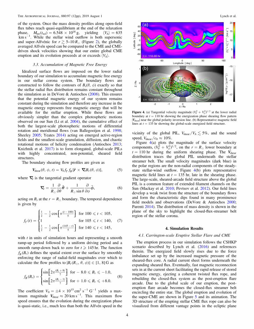
vicinity of the global PIL, V V 5%Ashear , and the soundspeed, »V c 10%shear 0 .Figure 4(a) plots the magnitude of the surface velocity

components, +q fV V2 2 1 2( ) , on the r=Re lower boundary att=110hr during the uniform shearing phase. The Vsheardistribution traces the global PIL underneath the stellarstreamer belt. The small velocity magnitudes (dark blue) inthe polar regions are the non-radial components of the steady-state stellar-wind outflow. Figure 4(b) plots representativemagnetic field lines at t=135hr, late in the shearing phase.The large-scale, sheared-arcade field structure above the globalPIL is a common feature of extended filament channels on theSun (Mackay et al. 2010; Pevtsov et al. 2012). Our field linesdevelop a weak twist from the structure of the boundary flowsand form the characteristic dips found in many prominencefield models and observations (DeVore & Antiochos 2000;Parenti 2014). The distribution of mass density is shown in theplane of the sky to highlight the closed-flux-streamer beltregion of the stellar corona.

4. Simulation Results

4.1. Carrington-scale Eruptive Stellar Flare and CME

The eruption process in our simulation follows the CSHKPscenario described by Lynch et al. (2016) and referencestherein. The energized field slowly rises due to the forceimbalance set up by the increased magnetic pressure of thesheared-flux core. A radial current sheet forms underneath theexpanding sheared flux. Eventually, fast magnetic reconnectionsets in at the current sheet facilitating the rapid release of storedmagnetic energy, ejecting a coherent twisted flux rope, andrebuilding the closed-flux system as the post-eruption flarearcade. Due to the global scale of our eruption, the post-eruption flare arcade becomes the closed-flux streamer beltencircling the entire star. The global eruption and evolution ofthe super-CME are shown in Figure 5 and its animation. The3D structure of the erupting stellar CME flux rope can also bevisualized from different vantage points in the ecliptic plane

Figure 4. (a) Tangential velocity magnitude +q fV V2 2 1 2( ) at the lower radialboundary at t=110hr showing the energization phase shearing flow patternVshear∣ ∣ near the global polarity inversion line. (b) Representative magnetic fieldlines at t=135hr showing the global-scale energized field structure.

4

The Astrophysical Journal, 880:97 (12pp), 2019 August 1 Lynch et al.

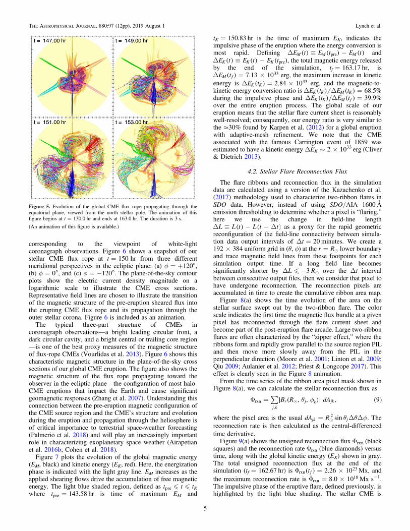
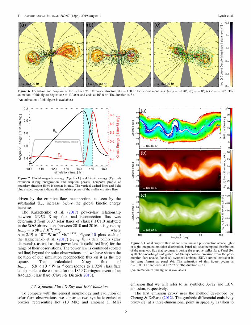
corresponding to the viewpoint of white-lightcoronagraph observations. Figure 6 shows a snapshot of ourstellar CME flux rope at t=150hr from three differentmeridional perspectives in the ecliptic plane: (a) f=+120°,(b) f=0°, and (c) f=−120°. The plane-of-the-sky contourplots show the electric current density magnitude on alogarithmic scale to illustrate the CME cross sections.Representative field lines are chosen to illustrate the transitionof the magnetic structure of the pre-eruption sheared flux intothe erupting CME flux rope and its propagation through theouter stellar corona. Figure 6 is included as an animation.

The typical three-part structure of CMEs incoronagraph observations—a bright leading circular front, adark circular cavity, and a bright central or trailing core region—is one of the best proxy measures of the magnetic structureof flux-rope CMEs (Vourlidas et al. 2013). Figure 6 shows thischaracteristic magnetic structure in the plane-of-the-sky crosssections of our global CME eruption. The figure also shows themagnetic structure of the flux rope propagating toward theobserver in the ecliptic plane—the configuration of most halo-CME eruptions that impact the Earth and cause significantgeomagnetic responses (Zhang et al. 2007). Understanding thisconnection between the pre-eruption magnetic configuration ofthe CME source region and the CME’s structure and evolutionduring the eruption and propagation through the heliosphere isof critical importance to terrestrial space-weather forecasting(Palmerio et al. 2018) and will play an increasingly importantrole in characterizing exoplanetary space weather (Airapetianet al. 2016b; Cohen et al. 2018).

Figure 7 plots the evolution of the global magnetic energy(EM, black) and kinetic energy (EK, red). Here, the energizationphase is indicated with the light gray line. EM increases as theapplied shearing flows drive the accumulation of free magneticenergy. The light blue shaded region, defined as tpre�t�tKwhere tpre=143.58 hr is time of maximum EM and

tK=150.83 hr is the time of maximum EK, indicates theimpulsive phase of the eruption where the energy conversion ismost rapid. Defining D º -E t E t E tM M Mpre( ) ( ) ( ) andD º -E t E t E tK K K pre( ) ( ) ( ), the total magnetic energy releasedby the end of the simulation, tf=163.17 hr, isD = ´E t 7.13 10M f

33( ) erg, the maximum increase in kineticenergy is D = ´E t 2.84 10K K

33( ) erg, and the magnetic-to-kinetic energy conversion ratio isD D =E t E t 68.5%K K M K( ) ( )during the impulsive phase and D D =E t E t 39.9%K K M f( ) ( )over the entire eruption process. The global scale of oureruption means that the stellar flare current sheet is reasonablywell-resolved; consequently, our energy ratio is very similar tothe ≈30% found by Karpen et al. (2012) for a global eruptionwith adaptive-mesh refinement. We note that the CMEassociated with the famous Carrington event of 1859 wasestimated to have a kinetic energyΔEK∼2×1033 erg (Cliver& Dietrich 2013).

4.2. Stellar Flare Reconnection Flux

The flare ribbons and reconnection flux in the simulationdata are calculated using a version of the Kazachenko et al.(2017) methodology used to characterize two-ribbon flares inSDO data. However, instead of using SDO/AIA 1600Åemission thresholding to determine whether a pixel is “flaring,”here we use the change in field-line lengthD º - - DL L t L t t( ) ( ) as a proxy for the rapid geometricreconfiguration of the field-line connectivity between simula-tion data output intervals of Δt=20 minutes. We create a192×384 uniform grid in (θ, f) at the r=Re lower boundaryand trace magnetic field lines from these footpoints for eachsimulation output time. If a long field line becomessignificantly shorter by ΔL�−3 Re over the Δt intervalbetween consecutive output files, then we consider that pixel tohave undergone reconnection. The reconnection pixels areaccumulated in time to create the cumulative ribbon area map.Figure 8(a) shows the time evolution of the area on the

stellar surface swept out by the two-ribbon flare. The colorscale indicates the first time the magnetic flux bundle at a givenpixel has reconnected through the flare current sheet andbecome part of the post-eruption flare arcade. Large two-ribbonflares are often characterized by the “zipper effect,” where theribbons form and rapidly grow parallel to the source region PILand then move more slowly away from the PIL in theperpendicular direction (Moore et al. 2001; Linton et al. 2009;Qiu 2009; Aulanier et al. 2012; Priest & Longcope 2017). Thiseffect is clearly seen in the Figure 8 animation.From the time series of the ribbon area pixel mask shown in

Figure 8(a), we can calculate the stellar reconnection flux as

å q fF = B R dA, , , 9j k

r j k jkrxn,

∣ ( )∣ ( )

where the pixel area is the usual q q f= D DdA R sinjk j2 . The

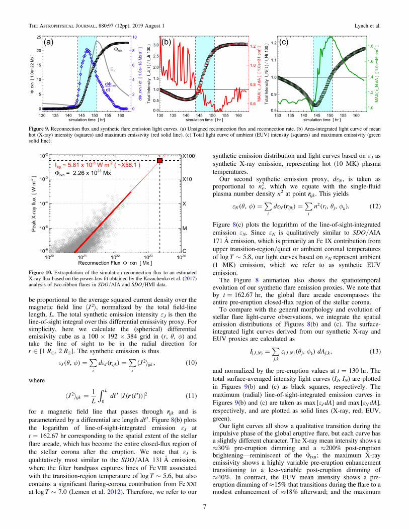
reconnection rate is then calculated as the central-differencedtime derivative.Figure 9(a) shows the unsigned reconnection flux Φrxn (black

squares) and the reconnection rate Frxn˙ (blue diamonds) versus

time, along with the global kinetic energy (EK) shown in gray.The total unsigned reconnection flux at the end of thesimulation (tf=162.67 hr) is F = ´t 2.26 10frxn

23( ) Mx, andthe maximum reconnection rate is F = ´8.0 10rxn

18˙ Mxs−1.The impulsive phase of the eruptive flare, defined previously, ishighlighted by the light blue shading. The stellar CME is

Figure 5. Evolution of the global CME flux rope propagating through theequatorial plane, viewed from the north stellar pole. The animation of thisfigure begins at t=130.0 hr and ends at 163.0 hr. The duration is 3 s.

(An animation of this figure is available.)

5

The Astrophysical Journal, 880:97 (12pp), 2019 August 1 Lynch et al.

driven by the eruptive flare reconnection, as seen by thesubstantial Frxn

˙ increase before the global kinetic energyincrease.

The Kazachenko et al. (2017) power-law relationshipbetween GOES X-ray flux and reconnection flux wasdetermined from 3137 solar flares of classes �C1.0 analyzedin the SDO observations between 2010 and 2016. It is given by

a= FI 10X ray rxn21 1.454( )‐ , where

α=2.19×10−6 Wm−2Mx−1.454. Figure 10 plots each ofthe Kazachenko et al. (2017) FI ,X ray rxn( )‐ data points (graydiamonds), as well as the power-law fit (solid red line) for therange of their observations. The power law is continued (dottedred line) beyond the solar observations, and we have shown thelocation of our simulation reconnection flux on it as the redsquare. The calculated X-ray flux ofIX‐ray=5.8×10−3 Wm−2 corresponds to a X58 class flarecomparable to the estimate for the 1859 Carrington event of anX45(±5) class flare (Cliver & Dietrich 2013).

4.3. Synthetic Flare X-Ray and EUV Emission

To compare with the general morphology and evolution ofsolar flare observations, we construct two synthetic emissionproxies representing hot (10 MK) and ambient (1 MK)

emission that we will refer to as synthetic X-ray and EUVemission, respectively.The first emission proxy uses the method developed by

Cheung & DeRosa (2012). The synthetic differential emissivityproxy ed J at a three-dimensional point in space rijk is taken to

Figure 6. Formation and eruption of the stellar CME flux-rope structure at t=150hr for central meridians: (a) f=+120°; (b) f=0°; (c) f=−120°. Theanimation of this figure begins at t=130.0 hr and ends at 163.0 hr. The duration is 3 s.

(An animation of this figure is available.)

Figure 7. Global magnetic energy (EM, black) and kinetic energy (EK, red)evolution during energization and eruption phases. Temporal profile ofboundary shearing flows is shown in gray. The vertical dashed lines and lightblue shaded region indicate the impulsive phase of the stellar eruptive flare.

Figure 8. Global eruptive flare ribbon structure and post-eruption arcade light-of-sight-integrated emission distribution. Panel (a): spatiotemporal distributionof the magnetic flux that reconnects during the eruptive stellar flare. Panel (b):synthetic line-of-sight-integrated hot (X-ray) coronal emission from the post-eruption flare arcade. Panel (c): synthetic ambient (EUV) coronal emission inthe same format as panel (b). The animation of this figure begins att=130.33 hr and ends at 162.67 hr. The duration is 3 s.

(An animation of this figure is available.)

6

The Astrophysical Journal, 880:97 (12pp), 2019 August 1 Lynch et al.

be proportional to the average squared current density over themagnetic field line á ñJ2 , normalized by the total field-linelength, L. The total synthetic emission intensity εJ is then theline-of-sight integral over this differential emissivity proxy. Forsimplicity, here we calculate the (spherical) differentialemissivity cube as a 100×192×384 grid in (r, θ, f) andtake the line of sight to be in the radial direction forÎr R R1 , 2[ ] . The synthetic emission is thus

å åe q f e= = á ñrd J, , 10Ji

J ijki

ijk2( ) ( ) ( )

where

òá ñ = ¢ ¢rJL

dℓ J ℓ1

11ijk

L2

0

2∣ ( ( ))∣ ( )

for a magnetic field line that passes through rijk and isparameterized by a differential arc length ¢dℓ . Figure 8(b) plotsthe logarithm of line-of-sight-integrated emission εJ att=162.67hr corresponding to the spatial extent of the stellarflare arcade, which has become the entire closed-flux region ofthe stellar corona after the eruption. We note that εJ isqualitatively most similar to the SDO/AIA 131Å emission,where the filter bandpass captures lines of Fe VIII associatedwith the transition-region temperature of ~Tlog 5.6, but alsocontains a significant flaring-corona contribution from Fe XXIat ~Tlog 7.0 (Lemen et al. 2012). Therefore, we refer to our

synthetic emission distribution and light curves based on εJ assynthetic X-ray emission, representing hot (10 MK) plasmatemperatures.Our second synthetic emission proxy, ed N , is taken as

proportional to ne2, which we equate with the single-fluid

plasma number density n2 at point rijk. This yields

å åe q f e q f= =rd n r, , , . 12Ni

N ijki

i j k2( ) ( ) ( ) ( )

Figure 8(c) plots the logarithm of the line-of-sight-integratedemission εN. Since εN is qualitatively similar to SDO/AIA171Å emission, which is primarily an FeIX contribution fromupper transition-region/quiet or ambient coronal temperaturesof ~Tlog 5.8, our light curves based on εN represent ambient(1 MK) emission, which we refer to as synthetic EUVemission.The Figure 8 animation also shows the spatiotemporal

evolution of our synthetic flare emission proxies. We note thatby t=162.67hr, the global flare arcade encompasses theentire pre-eruption closed-flux region of the stellar corona.To compare with the general morphology and evolution of

stellar flare light-curve observations, we integrate the spatialemission distributions of Figures 8(b) and (c). The surface-integrated light curves derived from our synthetic X-ray andEUV proxies are calculated as

å e q f=I dA, , 13J Nj k

J N j k j k,,

, ,( ) ( ){ } { }

and normalized by the pre-eruption values at t=130hr. Thetotal surface-averaged intensity light curves (IJ, IN) are plottedin Figures 9(b) and (c) as black squares, respectively. Themaximum (radial) line-of-sight-integrated emission curves inFigures 9(b) and (c) are taken as e dAmax J[ ] and e dAmax N[ ],respectively, and are plotted as solid lines (X-ray, red; EUV,green).Our light curves all show a qualitative transition during the

impulsive phase of the global eruptive flare, but each curve hasa slightly different character. The X-ray mean intensity shows a≈30% pre-eruption dimming and a ≈200% post-eruptionbrightening—reminiscent of the F ;rxn the maximum X-rayemissivity shows a highly variable pre-eruption enhancementtransitioning to a less-variable post-eruption dimming of≈40%. In contract, the EUV mean intensity shows a pre-eruption dimming of ≈15% that transitions during the flare to amodest enhancement of ≈18% afterward; and the maximum

Figure 9. Reconnection flux and synthetic flare emission light curves. (a) Unsigned reconnection flux and reconnection rate. (b) Area-integrated light curve of meanhot (X-ray) intensity (squares) and maximum emissivity (red solid line). (c) Total light curve of ambient (EUV) intensity (squares) and maximum emissivity (greensolid line).

Figure 10. Extrapolation of the simulation reconnection flux to an estimatedX-ray flux based on the power-law fit obtained by the Kazachenko et al. (2017)analysis of two-ribbon flares in SDO/AIA and SDO/HMI data.

7

The Astrophysical Journal, 880:97 (12pp), 2019 August 1 Lynch et al.

EUV emissivity shows the sharpest rise just after the onset ofthe flare, an ≈80% enhancement, and the clearest post-eruptiondecay. We note that while solar and stellar X-ray and EUVobservations measure the combined temperature and densityevolution during flares, the synthetic emission from ourisothermal simulation is determined solely by the densitycomponent.

Stellar flare observations in X-ray, UV, optical, and radiowavelengths are generally consistent with the CSHKP under-standing of eruptive solar flares (Hawley et al. 1995; Güdelet al. 2002; Osten & Wolk 2015). Harra et al. (2016) discussedthe solar SDO/EVE disk-integrated light curves of Fe ionspectral lines for signatures that could be applied to stellar flareobservations. They found that the lower ionization states of Feshow prompt dimming curves, whereas the higher ionizationstates show a rapid increase followed by a slow decay. Thestellar observations of pre-flare dimming have competingphysical interpretations (Leitzinger et al. 2014; Osten &Wolk 2017). The origin of the pre-flare dimming in our meanintensity light curves can be understood from the spatiotem-poral evolution of the emission distributions shown in theFigure 8 animation. As the pre-eruption closed-flux regionsexpand and the outer layers open into the stellar wind, theemission from the streamer belt decreases gradually. This isfollowed by the rapid CME-related dimming due to theeruption/opening-up of most of the remaining closed flux oncethe flare reconnection begins in earnest. The eruption-relateddimming is coincident with the initial formation of the flarearcade that has significantly enhanced emission compared tothe pre-flare configuration. As the post-eruption flare arcadegrows, its enhanced emission becomes the dominant feature ofthe global mean intensity light curves.

4.4. Stellar CME and CME-driven Shock Parameters

CMEs are responsible for some of the most geoeffectivespace-weather impacts at Earth and other solar system bodies.The combination of southward-directed Bz in the sheath andejecta flux rope with the increased dynamic pressure in densesheath regions driven by fast events can cause significantgeomagnetic responses (Zhang et al. 2007; Li et al. 2018). FastCMEs drive shocks, and these coronal and interplanetaryshocks are often sites of substantial energetic particleacceleration (Lario et al. 2016; Luhmann et al. 2018). Oursimulation results can be used to begin an investigation of

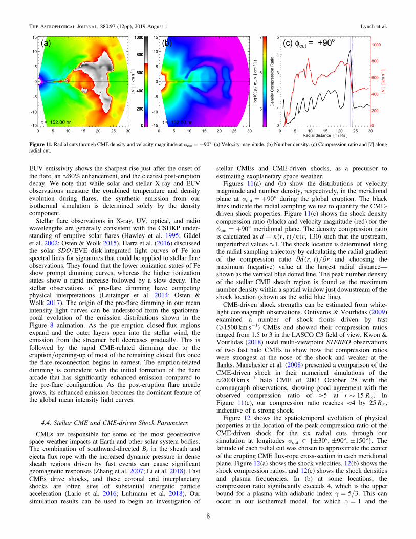
stellar CMEs and CME-driven shocks, as a precursor toestimating exoplanetary space weather.Figures 11(a) and (b) show the distributions of velocity

magnitude and number density, respectively, in the meridionalplane at fcut=+90° during the global eruption. The blacklines indicate the radial sampling we use to quantify the CME-driven shock properties. Figure 11(c) shows the shock densitycompression ratio (black) and velocity magnitude (red) for thefcut=+90° meridional plane. The density compression ratiois calculated as =d n r t n r, , 130( ) ( ) such that the upstream,unperturbed values ≈1. The shock location is determined alongthe radial sampling trajectory by calculating the radial gradientof the compression ratio ¶ ¶d r t r,( ) and choosing themaximum (negative) value at the largest radial distance—shown as the vertical blue dotted line. The peak number densityof the stellar CME sheath region is found as the maximumnumber density within a spatial window just downstream of theshock location (shown as the solid blue line).CME-driven shock strengths can be estimated from white-

light coronagraph observations. Ontiveros & Vourlidas (2009)examined a number of shock fronts driven by fast(�1500 km s−1) CMEs and showed their compression ratiosranged from 1.5 to 3 in the LASCO C3 field of view. Kwon &Vourlidas (2018) used multi-viewpoint STEREO observationsof two fast halo CMEs to show how the compression ratioswere strongest at the nose of the shock and weaker at theflanks. Manchester et al. (2008) presented a comparison of theCME-driven shock in their numerical simulations of the≈2000 km s−1 halo CME of 2003 October 28 with thecoronagraph observations, showing good agreement with theobserved compression ratio of ≈5 at ~r R15 . InFigure 11(c), our compression ratio reaches ≈4 by 25 Re,indicative of a strong shock.Figure 12 shows the spatiotemporal evolution of physical

properties at the location of the peak compression ratio of theCME-driven shock for the six radial cuts through oursimulation at longitudes fcut ä {±30°,±90°,±150°}. Thelatitude of each radial cut was chosen to approximate the centerof the erupting CME flux-rope cross-section in each meridionalplane. Figure 12(a) shows the shock velocities, 12(b) shows theshock compression ratios, and 12(c) shows the shock densitiesand plasma frequencies. In (b) at some locations, thecompression ratio significantly exceeds 4, which is the upperbound for a plasma with adiabatic index γ=5/3. This canoccur in our isothermal model, for which γ=1 and the

Figure 11. Radial cuts through CME density and velocity magnitude at fcut=+90°. (a) Velocity magnitude. (b) Number density. (c) Compression ratio and V∣ ∣ alongradial cut.

8

The Astrophysical Journal, 880:97 (12pp), 2019 August 1 Lynch et al.

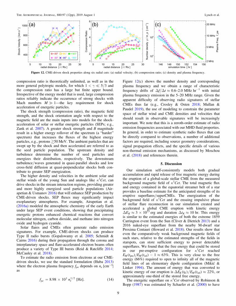
compression ratio is theoretically unlimited, as well as in themore general polytropic models, for which 1<γ=5/3 andthe compression ratio has a large but finite upper bound.Irrespective of the energy model that is used, large compressionratios reliably indicate the occurrence of strong shocks withMach numbers M?1—the key requirement for shockacceleration of energetic particles.

The shock strength (compression ratio), the magnetic fieldstrength, and the shock orientation angle with respect to themagnetic field are the main inputs into models for the shock-acceleration of solar or stellar energetic particles (SEPs; e.g.,Zank et al. 2007). A greater shock strength and B magnituderesult in a higher energy rollover of the spectrum (a “harder”spectrum) that increases the fluxes of the highest energyparticles, e.g., protons 50MeV. The ambient particles that areswept up by the shock and then accelerated are referred to asthe seed particle population. The upstream density andturbulence determine the number of seed particles andenergizes their distribution, respectively. The downstreamturbulence/waves generated in quasi-parallel shocks and lowcross-field diffusion at quasi-perpendicular shocks both con-tribute to greater SEP energization.

The higher density and velocities in the ambient solar andstellar winds of the young Sun and analogs like κ1Cet, candrive shocks in the stream interaction regions, providing greaterand more highly energized seed particle populations (Air-apetian & Usmanov 2016) that will enhance SEP production byCME-driven shocks. SEP fluxes may significantly impactexoplanetary atmospheres. For example, Airapetian et al.(2016a) modeled the atmospheric chemistry of the early Earthunder large SEP event conditions, showing that precipitatingenergetic protons enhanced chemical reactions that convertmolecular nitrogen, carbon dioxide, and methane into nitrogenoxide and hydrogen cyanide.

Solar flares and CMEs often generate radio emissionsignatures. For example, CME-driven shocks can produceType II radio bursts (Gopalswamy et al. 2005; Schmidt &Cairns 2016) during their propagation through the corona andinterplanetary space and flare-accelerated electron beams oftenproduce a variety of Type III bursts (Reid & Ratcliffe 2014;McCauley et al. 2018).

To estimate the radio emission from electrons at our CME-driven shocks, we use the standard formulation (Huba 2013)where the electron plasma frequency fpe depends on ne -cm 3[ ]as

= ´f n8.98 10 Hz . 14pe e3 1 2 [ ] ( )

Figure 12(c) shows the number density and correspondingplasma frequency and we obtain a range of characteristicfrequency drifts of Δf/Δt≈0.6–2.0MHzhr−1 with initialplasma frequency emission in the 5–20MHz range. Given theapparent difficulty of observing radio signatures of stellarCMEs thus far (e.g., Crosley & Osten 2018; Mullan &Paudel 2019), the use of modeling to constrain the parameterspace of stellar wind and CME densities and velocities thatshould result in observable signatures will be increasinglyimportant. We note that this is a zeroth-order estimate of radioemission frequencies associated with our MHD fluid properties.In general, in order to estimate synthetic radio fluxes that canbe directly compared to observations, a number of additionalfactors are required, including source geometry considerations,signal propagation effects, and the specific details of variousnon-thermal emission mechanisms, as discussed by Moschouet al. (2018) and references therein.

5. Discussion

Our simulation self-consistently models both gradualaccumulation and rapid release of free magnetic energy duringthe eruption of a global-scale stellar CME from the measuredbackground magnetic field of κ1Cet. The total magnetic fluxand energy contained in the equatorial streamer belt of a starprovides a baseline estimate for the anticipated strengths of itseruptive superflares/superCMEs. The energization of thebackground field of κ1Cet and the ensuing impulsive phaseof stellar flare reconnection in our simulation created andaccelerated a global CME eruption with kinetic energyΔEK≈3×1033 erg and duration ΔtK≈10hr. This energyis similar to the estimated energies of both the extreme 1859Carrington event from the Sun (Cliver & Dietrich 2013) and a2016 naked-eye superflare from the nearby M-dwarf starProxima Centauri (Howard et al. 2018). Our results show thateven the comparatively weak background magnetic fields ofsuch stars, relative to the estimated strengths of the fields instarspots, can store sufficient energy to power detectablesuperflares. We found that the free energy that could be storedin our pre-eruptive configuration for κ1Cet reached

- »E t E t 1 63%M Mpre rel( ) ( ) . This is very close to the freeenergy (66%) required to open to infinity all of the magneticfield lines of an elementary dipole configuration (Mikić &Linker 1994). The amount of energy that was converted tokinetic energy of our eruption is D »E t E t 22%K K M rel( ) ( ) , orapproximately one-third of the stored free energy.The energetic superflare on κ1Cet observed by Robinson &

Bopp (1987) was estimated by Schaefer et al. (2000) to have

Figure 12. CME-driven shock properties along six radial cuts: (a) radial velocity; (b) compression ratio; (c) density and plasma frequency.

9

The Astrophysical Journal, 880:97 (12pp), 2019 August 1 Lynch et al.

released about 2×1034 erg, an order of magnitude moreenergy than our simulated event from the recently measuredbackground magnetic field of the star (Rosén et al. 2016). It isinteresting to note that the energy of the observed 1986 κ1Cetsuperflare is roughly twice the energy contained within itsbackground field, 2×1034 erg versus 1×1034 erg (seeFigure 3). Correspondingly, the estimated energy of thehistoric Carrington 1859 solar flare (Cliver & Dietrich 2013)and the energy of the Sun’s present-day background field(Yeates et al. 2018) are each smaller by about one order ofmagnitude, 2×1033 erg versus 1×1033 erg. The similarity inthe flare-to-background energy ratio suggests that the Robin-son-Bopp superflare on κ1Cet may have been as extreme anevent for that star as the Carrington flare was for the Sun.Verifying this correspondence would require obtaining andanalyzing a long-duration database of flare observations ofκ1Cet and similar stars. Encouragingly, Notsu et al. (2019) andcollaborators are investigating precisely this subset of super-flaring solar-type stars in the Kepler data.

There are two primary areas where our idealized modelingcould be improved upon in future numerical simulations. First,the magnetic flux distribution in the ZDI stellar magnetogramcaptures the global structure of the background magnetic fieldbut does not resolve the field strengths or spatial scalesassociated with starspots or active regions. Second, theisothermal model for the stellar atmosphere does not accountfor the full thermodynamic evolution of the plasma, whichaffects the density and temperature distribution of the back-ground wind and also means that the flare-related energydeposition into bulk plasma heating during the eruption is notcaptured in the simulation. We discuss each of these issues, inturn, below.

Our energization process imparts shear and twist to thecoronal field structure in exactly the place the Sun requires (i.e.,localized above the PIL). This enables the system both togradually accumulate free energy and to transition rapidly to anunstable, runaway eruption that removes this localized stressedfield from the closed-field corona via magnetic reconnection.Thus, the energization and eruption-triggering processes in oursimulation are completely generic and should be universallyapplicable, including to more realistic solar and stellarmagnetic field configurations.

More realistic stellar active-region fields will be stronger(100s–1000s G) and significantly more localized spatially,although potentially over areas larger than observed on theSun. For example, Rucinski et al. (2004) used the Micro-variability and Oscillations of Stars observations of κ1Cet toderive the sizes of two large starspots that covered 1.4% and3.6% of the stellar surface, respectively. These areas areroughly 10 times greater that the largest sunspot/AR areas everobserved on the Sun (Hoge 1947). The magnetic energyestimates used in stellar flare analyses are typically of the form

p~E B A1 8M AR2

AR3 2( ( )) (e.g., Shibata et al. 2013; Maehara

et al. 2015; Notsu et al. 2019). If we were to scale the magneticenergy of our system, ~ ´E t 1.3 10M rel

34( ) erg, to astarspot area estimate of p~ A f RAR

2( ) wheref=0.002–0.02, then we obtain a range of areasAAR=3×1019–20 cm2 and a resulting range of starspot/ARfield strengths, BAR∼250–1400 G. These field strengths arecomfortably within the range of both solar observations (e.g.,Figure 10 of Kazachenko et al. 2017) and the Saar & Baliunas

(1992) estimate of 350–500 G for the κ1Cet surface-averagedfield magnitudes.We emphasize that our approach represents an attempt to

model the most extreme stellar space-weather event possiblewithin the observational constraints imposed by the surfacemagnetic flux distribution from the ZDI reconstruction. Despitethe global spatial scale and the stellar magnetogram’sunresolved starspot/AR flux distribution, the magnetic energystored and released in our simulation’s eruptive superflare iscompatible with the order-of-magnitude estimate one obtainsfrom typical starspot/AR areas and magnetic field strengths.On the other hand, if much stronger unresolved starspots/ARflux distributions were assumed, the resulting superflare andsuper-CME energies could be much higher. For example,recent analyses by Okamoto & Sakurai (2018) of Hinodespectropolarimetry data of NOAA AR 11967 in 2014 February1–6 showed a peak magnetic field strength of 6.2kG. Thissolar magnetic field magnitude over the range of starspot/ARareas above would result in much larger magnetic energyestimates of EM∼2.5×1035–8×1036 erg.Our use of an isothermal stellar atmosphere neglects the

internal energy equation in the MHD system and consequently,the evolution of our gas pressure is determined solely by thevariation in mass density. In more complex thermodynamicMHD models, the internal energy equation typically includesfield-aligned heat conduction, radiative cooling, magnetic andviscous dissipation, and a source term for the local contributionfrom coronal heating. One such parameterized coronal heatingmodel represents the dissipation of energy associated withAlfvénic turbulence, which contributes both to local plasmaheating, and through the wave pressure gradient, to theacceleration of the solar wind (Lionello et al. 2014; van derHolst et al. 2014; Oran et al. 2017). While a polytropic stellarwind outflow naturally creates a significant mass densitygradient between the open-flux regions (coronal holes) and theclosed-field corona (the helmet streamer belt), a more realistictreatment of the internal energy equation is expected to increasethis density contrast for both the quiet-Sun and active regions(e.g., Török et al. 2018). The isothermal model for our stellaratmosphere has two main consequences for our simulationresults: first, on the structure and intensities associated with oursynthetic EUV and soft X-ray emission profiles; second, on theinteraction between the CME and the background wind,including the properties of the CME-driven shock.As discussed above, approximately one-third of the free

magnetic energy stored prior to the eruption is converted tokinetic energy of the CME. About one-sixth of the storedenergy remained in the closed coronal field after the eruption;that is, the magnetic field did not relax completely to the initial,minimum-energy state of the system. The remaining energyreleased by the magnetic field during the eruption,D »E E t 32%H M rel( ) of the initial magnetic energy, was notcaptured by our simple isothermal model. This remnantreleased energy ΔEH would appear as thermal energy due tomagnetic and viscous dissipation, heating the stellar plasma tohigh flare temperatures and being radiated away into space.With a more realistic temperature structure in the dynamicformation and evolution of the flare current sheet and the post-eruption arcade (e.g., Reeves et al. 2010; Lynch et al. 2011),one could improve the synthetic emission calculations ofSection 4.3 by calculating the density- and temperature-dependent emission intensities in various spectral lines and

10

The Astrophysical Journal, 880:97 (12pp), 2019 August 1 Lynch et al.

convolving these with instrument response functions (e.g.,Lionello et al. 2009; Reeves et al. 2010; Shen et al. 2013; Jinet al. 2017; Oran et al. 2017).

Relaxing the isothermal assumption would result in amodified stellar wind profile, and thus, quantitative differencesin the plasma properties of the CME–stellar wind interactionregion. Qualitatively, the overall picture will remain the sameas in Figure 11, i.e., the energetic eruption driven by the flarereconnection will create and accelerate a rapidly expanding,highly magnetized (low β) flux-rope ejecta that will generate ashock and a dense compression region at the CME’s leadingedge. A modified upstream stellar wind profile will obviouslyimpact the absolute number densities and an improvedthermodynamic treatment will allow for additional localized,compressional heating. The shock is expected to remainAlfvénic; however, detailed shock parameters such as thecompression ratio, field strength, and the shock normalorientation will have different quantitative values. Even withthe simple isothermal model used here, the compression ratiosgenerated in our simulation are broadly consistent with thosedetermined from the white-light coronagraph observations oflarge solar events.

Therefore, limitations notwithstanding, our simulationresults represent an important step toward understandingobservations of superflares from active solar-type stars andcharacterizing CMEs from magnetically active stars across theK–M dwarf-star spectrum. We analyzed the properties ofCME-induced shocks, including the frequency and duration ofassociated Type II events that may be detected in future low-frequency (10 MHz or lower) radio observations of magneti-cally active stars. The derived properties of CMEs and theirassociated shocks can provide inputs to models of stellar SEPenergization and transport via the diffusive shock-accelerationmechanism (Li et al. 2013; Hu et al. 2018). Knowledge of theSEP energy spectrum and particle fluence is critical forevaluating biogenic conditions on terrestrial-type exoplanetsaround active stars, as well as for the early Earth and Mars.Airapetian et al. (2016b) have shown that large SEP fluxes canincrease the production rates of nitrous oxide, a powerfulgreenhouse gas, and hydrogen cyanide, a feedstock moleculefor prebiotic synthesis. Characterizing the SEP environmentwill help to determine the boundaries of the planetary“biogenic” zone (Airapetian et al. 2019a) and will be importantin specifying the efficiency of ozone destruction and surfacedosages of ionizing radiation that are damaging to life onplanetary surfaces. Future modeling efforts that describe theconditions of CME initiation in more realistic stellar magneticfield distributions can help us to understand observations of G,K, and M dwarf stars using the currently implementedinternational multi-observatory program (TESS, Hubble,XMM-Newton, Apache Point Observatory) and to prepare fornext-generation JWST observations.

B.J.L., M.D.K., and W.P.A. acknowledge support fromNASA NNX17AI28G, NSF AGS-1622495, and the CoronalGlobal Evolutionary Model (CGEM) project NSF AGS-1321474. V.S.A. acknowledges support from the NASAExobiology 80NSSC17K0463 and the TESS 1 Cycle 1program. C.R.D. acknowledges support from the NASAH-SR and LWS TR&T programs. T.L. acknowledges supportvia the Austrian Space Application Programme (ASAP) of theAustrian Research Promotion Agency (FFG) within ASAP11

and the FWF NFN project S11601-N16. O.K. acknowledgessupport by the Knut and Alice Wallenberg Foundation (projectgrant “The New Milky Way”), the Swedish Research Council(project 621-2014-5720), and the Swedish National SpaceBoard (projects 185/14, 137/17). The computational resourcesfor this work were provided to B.J.L. by the NASA High-EndComputing Program through the NASA Center for ClimateSimulation at Goddard Space Flight Center.

ORCID iDs

Benjamin J. Lynch https://orcid.org/0000-0001-6886-855XVladimir S. Airapetian https://orcid.org/0000-0003-4452-0588C. Richard DeVore https://orcid.org/0000-0002-4668-591XMaria D. Kazachenko https://orcid.org/0000-0001-8975-7605Oleg Kochukhov https://orcid.org/0000-0003-3061-4591

References

Airapetian, V., Glocer, A., & Gronoff, G. 2016a, in IAU Symp. 320, Solar andStellar Flares and their Effects on Planets, ed. A. G. Kosovichev,S. L. Hawley, & P. Heinzel (Cambridge: Cambridge Univ. Press), 409

Airapetian, V. S., Barnes, R., Cohen, O., et al. 2019a, IJAsB, in press(arXiv:1905.05093)

Airapetian, V. S., Glocer, A., Gronoff, G., Hébrard, E., & Danchi, W. 2016b,NatGe, 9, 452

Airapetian, V. S., Glocer, A., Khazanov, G. V., et al. 2017, ApJL, 836, L3Airapetian, V. S., Jin, M., Lüftinger, T., et al. 2019b, NatAs, submittedAirapetian, V. S., & Usmanov, A. V. 2016, ApJL, 817, L24Antiochos, S. K. 2013, ApJ, 772, 72Aulanier, G., Janvier, M., & Schmieder, B. 2012, A&A, 543, A110Carmichael, H. 1964, NASSP, 50, 451Cheung, M. C. M., & DeRosa, M. L. 2012, ApJ, 757, 147Cliver, E. W., & Dietrich, W. F. 2013, JSWSC, 3, A31Cohen, O., Drake, J. J., Glocer, A., et al. 2014, ApJ, 790, 57Cohen, O., Glocer, A., Garraffo, C., Drake, J. J., & Bell, J. M. 2018, ApJL,

856, L11Cohen, O., Kashyap, V. L., Drake, J. J., et al. 2011, ApJ, 733, 67Crosley, M. K., & Osten, R. A. 2018, ApJ, 856, 39DeVore, C. R. 1991, JCoPh, 92, 142DeVore, C. R., & Antiochos, S. K. 2000, ApJ, 539, 954DeVore, C. R., & Antiochos, S. K. 2008, ApJ, 680, 740Domagal-Goldman, S. D., Segura, A., Claire, M. W., Robinson, T. D., &

Meadows, V. S. 2014, ApJ, 792, 90do Nascimento, J.-D., Jr., Vidotto, A. A., Petit, P., et al. 2016, ApJL, 820, L15Donati, J.-F., & Brown, S. F. 1997, A&A, 326, 1135Dong, C., Lingam, M., Ma, Y., & Cohen, O. 2017, ApJL, 837, L26Drake, J. J., Cohen, O., Yashiro, S., & Gopalswamy, N. 2013, ApJ, 764, 170Emslie, A. G., Dennis, B. R., Shih, A. Y., et al. 2012, ApJ, 759, 71Fletcher, L., Dennis, B. R., Hudson, H. S., et al. 2011, SSRv, 159, 19Forbes, T. G. 2000, JGRA, 105, 23153Garcia-Sage, K., Glocer, A., Drake, J. J., Gronoff, G., & Cohen, O. 2017,

ApJL, 844, L13Garraffo, C., Drake, J. J., & Cohen, O. 2016, ApJL, 833, L4Garraffo, C., Drake, J. J., Cohen, O., Alvarado-Gómez, J. D., & Moschou, S. P.

2017, ApJL, 843, L33Gopalswamy, N., Aguilar-Rodriguez, E., Yashiro, S., et al. 2005, JGRA, 110,

A12S07Güdel, M., Audard, M., Skinner, S. L., & Horvath, M. I. 2002, ApJL, 580, L73Harra, L. K., Schrijver, C. J., Janvier, M., et al. 2016, SoPh, 291, 1761Hawley, S. L., Fisher, G. H., Simon, T., et al. 1995, ApJ, 453, 464Hirayama, T. 1974, SoPh, 34, 323Hoge, E. R. 1947, PASP, 59, 109Howard, W. S., Tilley, M. A., Corbett, H., et al. 2018, ApJL, 860, L30Hu, J., Li, G., Fu, S., Zank, G., & Ao, X. 2018, ApJL, 854, L19Huba, J. D. 2013, NRL PLASMA FORMULARY Supported by The Office of

Naval Research (Washington, DC: Naval Research Laboratory), 1Janvier, M., Aulanier, G., & Démoulin, P. 2015, SoPh, 290, 3425Jin, M., Manchester, W. B., van der Holst, B., et al. 2017, ApJ, 834, 172Karpen, J. T., Antiochos, S. K., & DeVore, C. R. 2012, ApJ, 760, 81Kay, C., Opher, M., Colaninno, R. C., & Vourlidas, A. 2016, ApJ, 827, 70

11

The Astrophysical Journal, 880:97 (12pp), 2019 August 1 Lynch et al.

Kazachenko, M. D., Canfield, R. C., Longcope, D. W., & Qiu, J. 2012, SoPh,277, 165

Kazachenko, M. D., Lynch, B. J., Welsch, B. T., & Sun, X. 2017, ApJ, 845, 49Klimchuk, J. A. 2001, GMS, 125, 143Knizhnik, K. J., Antiochos, S. K., & DeVore, C. R. 2017, ApJ, 835, 85Kochukhov, O. 2016, in Lecture Notes in Physics, Vol. 914 ed. J.-P. Rozelot &

C. Neiner (Berlin: Springer), 177Kopp, R. A., & Pneuman, G. W. 1976, SoPh, 50, 85Kwon, R.-Y., & Vourlidas, A. 2018, JSWSC, 8, A08Lammer, H., Bredehöft, J. H., Coustenis, A., et al. 2009, A&ARv, 17, 181Lammer, H., Lichtenegger, H. I. M., Kulikov, Y. N., et al. 2007, AsBio, 7, 185Lario, D., Kwon, R.-Y., Vourlidas, A., et al. 2016, ApJ, 819, 72Leitzinger, M., Odert, P., Greimel, R., et al. 2014, MNRAS, 443, 898Lemen, J. R., Title, A. M., Akin, D. J., et al. 2012, SoPh, 275, 17Li, G., Zank, G., Verkhoglyadova, O., & Ding, L. 2013, in SOLAR WIND 13:

Proceedings of the Thirteenth International Solar Wind Conference 1539,ed. G. Zank et al. (Melville, New York: AIP), 105

Li, Y., Luhmann, J., Fisher, G., & Welsch, B. 2004, JASTP, 66, 1271Li, Y., Luhmann, J. G., & Lynch, B. J. 2018, SoPh, 293, 135Linton, M. G., DeVore, C. R., & Longcope, D. W. 2009, EP&S, 61, 573Lionello, R., Linker, J. A., & Mikić, Z. 2009, ApJ, 690, 902Lionello, R., Velli, M., Downs, C., et al. 2014, ApJ, 784, 120Lüftinger, T., Fröhlich, H.-E., Weiss, W. W., et al. 2010a, A&A, 509, A43Lüftinger, T., Kochukhov, O., Ryabchikova, T., et al. 2010b, A&A, 509, A71Lüftinger, T., Vidotto, A. A., & Johnstone, C. P. 2015, in Characterizing Stellar

and Exoplanetary Environments, Vol. 411, ed. H. Lammer &M. Khodachenko (Cham: Springer), 37

Luhmann, J. G., Mays, M. L., Li, Y., et al. 2018, SpWea, 16, 557Lynch, B. J., Antiochos, S. K., DeVore, C. R., Luhmann, J. G., &

Zurbuchen, T. H. 2008, ApJ, 683, 1192Lynch, B. J., Masson, S., Li, Y., et al. 2016, JGRA, 121, 10677Lynch, B. J., Reinard, A. A., Mulligan, T., et al. 2011, ApJ, 740, 112Mackay, D. H., Karpen, J. T., Ballester, J. L., Schmieder, B., & Aulanier, G.

2010, SSRv, 151, 333MacNeice, P., Olson, K. M., Mobarry, C., de Fainchtein, R., & Packer, C.

2000, CoPhC, 126, 330Maehara, H., Shibayama, T., Notsu, S., et al. 2012, Natur, 485, 478Maehara, H., Shibayama, T., Notsu, Y., et al. 2015, EP&S, 67, 59Manchester, W. B., IV, Vourlidas, A., Tóth, G., et al. 2008, ApJ, 684, 1448McCauley, P. I., Cairns, I. H., & Morgan, J. 2018, SoPh, 293, 132Mikić, Z., & Linker, J. A. 1994, ApJ, 430, 898Moore, R. L., Sterling, A. C., Hudson, H. S., & Lemen, J. R. 2001, ApJ,

552, 833Moschou, S.-P., Sokolov, I., Cohen, O., et al. 2018, ApJ, 867, 51Mullan, D. J., & Paudel, R. R. 2019, ApJ, 873, 1Notsu, Y., Maehara, H., Honda, S., et al. 2019, ApJ, 876, 58Notsu, Y., Shibayama, T., Maehara, H., et al. 2013, ApJ, 771, 127Okamoto, T. J., & Sakurai, T. 2018, ApJL, 852, L16Ontiveros, V., & Vourlidas, A. 2009, ApJ, 693, 267

Oran, R., Landi, E., van der Holst, B., Sokolov, I. V., & Gombosi, T. I. 2017,ApJ, 845, 98

Osten, R. A., & Wolk, S. J. 2015, ApJ, 809, 79Osten, R. A., & Wolk, S. J. 2017, in IAU Symp. 328, Living Around Active

Stars, ed. D. Nandy, A. Valio, & P. Petit (Cambridge: Cambridge Univ.Press), 243

Palmerio, E., Kilpua, E. K. J., Möstl, C., et al. 2018, SpWea, 16, 442Parenti, S. 2014, LRSP, 11, 1Parker, E. N. 1958, ApJ, 128, 664Petit, P., Louge, T., Théado, S., et al. 2014, PASP, 126, 469Pevtsov, A. A., Panasenco, O., & Martin, S. F. 2012, SoPh, 277, 185Piskunov, N., & Kochukhov, O. 2002, A&A, 381, 736Priest, E. R., & Longcope, D. W. 2017, SoPh, 292, 25Qiu, J. 2009, ApJ, 692, 1110Reeves, K. K., Linker, J. A., Mikić, Z., & Forbes, T. G. 2010, ApJ, 721, 1547Reid, H. A. S., & Ratcliffe, H. 2014, RAA, 14, 773Ribas, I., Porto de Mello, G. F., Ferreira, L. D., et al. 2010, ApJ, 714, 384Robinson, C. R., & Bopp, B. W. 1987, in Cool Stars, Stellar Systems and the

Sun, Vol. 291, ed. J. L. Linsky & R. E. Stencel (Berlin: Springer), 509Rosén, L., Kochukhov, O., Hackman, T., & Lehtinen, J. 2016, A&A, 593, A35Rucinski, S. M., Walker, G. A. H., Matthews, J. M., et al. 2004, PASP,

116, 1093Rugheimer, S., Kaltenegger, L., Segura, A., Linsky, J., & Mohanty, S. 2015,

ApJ, 809, 57Saar, S. H., & Baliunas, S. L. 1992, in ASP Conf. Ser. 27, The Solar Cycle, ed.

K. L. Harvey (San Francisco, CA: ASP), 197Schaefer, B. E., King, J. R., & Deliyannis, C. P. 2000, ApJ, 529, 1026Schmidt, J. M., & Cairns, I. H. 2016, GeoRL, 43, 50Segura, A., Kasting, J. F., Meadows, V., et al. 2005, AsBio, 5, 706Sheeley, N. R., Jr. 2005, LRSP, 2, 5Shen, C., Reeves, K. K., Raymond, J. C., et al. 2013, ApJ, 773, 110Shibata, K., Isobe, H., Hillier, A., et al. 2013, PASJ, 65, 49Shibayama, T., Maehara, H., Notsu, S., et al. 2013, ApJS, 209, 5Sturrock, P. A. 1966, Natur, 211, 695Török, T., Downs, C., Linker, J. A., et al. 2018, ApJ, 856, 75van Ballegooijen, A. A., Cartledge, N. P., & Priest, E. R. 1998, ApJ, 501, 866van der Holst, B., Sokolov, I. V., Meng, X., et al. 2014, ApJ, 782, 81Vidotto, A. A., Fares, R., Jardine, M., et al. 2012, MNRAS, 423, 3285Vidotto, A. A., Jardine, M., Opher, M., Donati, J. F., & Gombosi, T. I. 2011,

MNRAS, 412, 351Vourlidas, A., Lynch, B. J., Howard, R. A., & Li, Y. 2013, SoPh, 284, 179Walker, G. A. H., Croll, B., Kuschnig, R., et al. 2007, ApJ, 659, 1611Wang, Y.-M., & Sheeley, N. R., Jr. 1992, ApJ, 392, 310Welsch, B. T. 2018, SoPh, 293, 113Yeates, A. R. 2014, SoPh, 289, 631Yeates, A. R., Amari, T., Contopoulos, I., et al. 2018, SSRv, 214, 99Zank, G. P., Li, G., & Verkhoglyadova, O. 2007, SSRv, 130, 255Zhang, J., Richardson, I. G., Webb, D. F., et al. 2007, JGRA, 112, A10102

12

The Astrophysical Journal, 880:97 (12pp), 2019 August 1 Lynch et al.