
Model Reduction (Approximation) of Large-Scale Systems ...
63
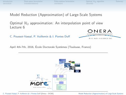
Introduction State-space formulation Poles-residues formulation Optimal H 2 algorithm Summary Model Reduction (Approximation) of Large-Scale Systems Optimal H 2 approximation: An interpolation point of view Lecture 6 C. Poussot-Vassal, P. Vuillemin & I. Pontes Duff April 4th-7th, 2016, École Doctorale Systèmes (Toulouse, France) more more Σ (A,B,C,D)i Σ ˆ Σ (ˆ A, ˆ B, ˆ C, ˆ D)i model reduction toolbox Kr(A, B) AP +PAT +BBT =0 WTV DAE/ODE State x(t) ∈Rn, n large or infinite Data Reduced DAE/ODE Reduced state ˆ x(t) ∈ Rr with r n (+) Simulation (+) Analysis (+) Control (+) Optimization Case 1 u(f)=[u(f1)...u(fi)] y(f)=[y(f1)...y(fi)] Case 2 E˙ x(t)=Ax(t)+Bu(t) y(t)=Cx(t)+Du(t) Case 3 H(s)=e-τs C. Poussot-Vassal, P. Vuillemin & I. Pontes Duff [Onera - DCSD] Model Reduction (Approximation) of Large-Scale Systems
Transcript of Model Reduction (Approximation) of Large-Scale Systems ...
Introduction State-space formulation Poles-residues formulation OptimalH2 algorithm Summary
Model Reduction (Approximation) of Large-Scale Systems
Optimal H2 approximation: An interpolation point of viewLecture 6
C. Poussot-Vassal, P. Vuillemin & I. Pontes Duff
April 4th-7th, 2016, École Doctorale Systèmes (Toulouse, France)
moremoreΣ
(A,B,C,D)i
Σ
Σ
(A, B, C, D)i
model reduction toolbox
Kr(A,B)
AP + PAT + BBT = 0
WTV
DAE/ODE
State x(t) ∈ Rn, n large orinfinite
Data
ReducedDAE/ODE
Reduced state x(t) ∈ Rrwith r � n(+) Simulation(+) Analysis(+) Control(+) Optimization
Case 1u(f) = [u(f1) . . . u(fi)]y(f) = [y(f1) . . . y(fi)]
Case 2Ex(t) = Ax(t) +Bu(t)y(t) = Cx(t) +Du(t)
Case 3H(s) = e−τs
C. Poussot-Vassal, P. Vuillemin & I. Pontes Duff [Onera - DCSD] Model Reduction (Approximation) of Large-Scale Systems
Introduction State-space formulation Poles-residues formulation OptimalH2 algorithm Summary
IntroductionThe projection-based frameworkObjectives of the lectureGeneral problem formulation
First-order optimality conditions: State-space approachProblem statementGradients of the errorLink with the projection framework
First-order optimality conditions: Poles-residues approachProblem statementGradients of the error
Fixed-point algorithm for optimal H2 reductionIdeaKey elements of the algorithmsIterative Tangential Interpolation Algorithm (ITIA)Example
Summary
C. Poussot-Vassal, P. Vuillemin & I. Pontes Duff [Onera - DCSD] Model Reduction (Approximation) of Large-Scale Systems
Introduction State-space formulation Poles-residues formulation OptimalH2 algorithm Summary
Outlines
IntroductionThe projection-based frameworkObjectives of the lectureGeneral problem formulation
First-order optimality conditions: State-space approach
First-order optimality conditions: Poles-residues approach
Fixed-point algorithm for optimal H2 reduction
Summary
C. Poussot-Vassal, P. Vuillemin & I. Pontes Duff [Onera - DCSD] Model Reduction (Approximation) of Large-Scale Systems
Introduction State-space formulation Poles-residues formulation OptimalH2 algorithm Summary
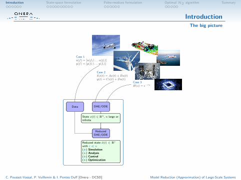
IntroductionThe big picture
C. Poussot-Vassal, P. Vuillemin & I. Pontes Duff [Onera - DCSD] Model Reduction (Approximation) of Large-Scale Systems
DAE/ODE
State x(t) ∈ Rn, n large orinfinite
Data
ReducedDAE/ODE
Reduced state x(t) ∈ Rrwith r � n(+) Simulation(+) Analysis(+) Control(+) Optimization
Case 1u(f) = [u(f1) . . . u(fi)]y(f) = [y(f1) . . . y(fi)]
Case 2Ex(t) = Ax(t) +Bu(t)y(t) = Cx(t) +Du(t)
Case 3H(s) = e−τs
Introduction State-space formulation Poles-residues formulation OptimalH2 algorithm Summary
IntroductionThe projection-based framework
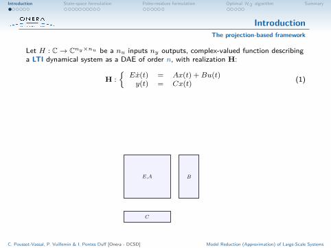
Let H : C→ Cny×nu be a nu inputs ny outputs, complex-valued function describinga LTI dynamical system as a DAE of order n, with realization H:
H :{
Ex(t) = Ax(t) +Bu(t)y(t) = Cx(t) (1)
C. Poussot-Vassal, P. Vuillemin & I. Pontes Duff [Onera - DCSD] Model Reduction (Approximation) of Large-Scale Systems
E,A B
C
Introduction State-space formulation Poles-residues formulation OptimalH2 algorithm Summary
IntroductionThe projection-based framework
Let H : C→ Cny×nu be a nu inputs ny outputs, complex-valued function describinga LTI dynamical system as a DAE of order n, with realization H:
H :{
Ex(t) = Ax(t) +Bu(t)y(t) = Cx(t) (1)
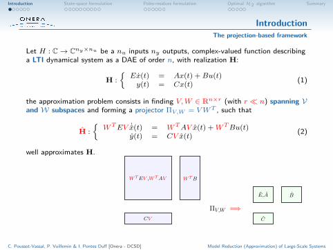
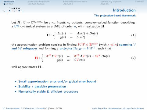
the approximation problem consists in finding V,W ∈ Rn×r (with r � n) spanning Vand W subspaces and forming a projector ΠV,W = VWT , such that
H :{
WTEV ˙x(t) = WTAV x(t) +WTBu(t)y(t) = CV x(t) (2)
well approximates H.
C. Poussot-Vassal, P. Vuillemin & I. Pontes Duff [Onera - DCSD] Model Reduction (Approximation) of Large-Scale Systems
WTEV ,WTAV WTB
CV
ΠV,W =⇒C
E,A B
Introduction State-space formulation Poles-residues formulation OptimalH2 algorithm Summary
IntroductionThe projection-based framework
Let H : C→ Cny×nu be a nu inputs ny outputs, complex-valued function describinga LTI dynamical system as a DAE of order n, with realization H:
H :{
Ex(t) = Ax(t) +Bu(t)y(t) = Cx(t) (1)
the approximation problem consists in finding V,W ∈ Rn×r (with r � n) spanning Vand W subspaces and forming a projector ΠV,W = VWT , such that
H :{
WTEV ˙x(t) = WTAV x(t) +WTBu(t)y(t) = CV x(t) (2)
well approximates H.
I Small approximation error and/or global error boundI Stability / passivity preservationI Numerically stable & efficient procedure
C. Poussot-Vassal, P. Vuillemin & I. Pontes Duff [Onera - DCSD] Model Reduction (Approximation) of Large-Scale Systems
Introduction State-space formulation Poles-residues formulation OptimalH2 algorithm Summary
IntroductionObjectives of the lecture
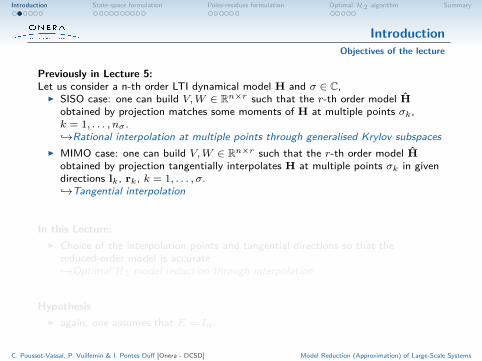
Previously in Lecture 5:Let us consider a n-th order LTI dynamical model H and σ ∈ C,
I SISO case: one can build V,W ∈ Rn×r such that the r-th order model Hobtained by projection matches some moments of H at multiple points σk,k = 1, . . . , nσ .↪→Rational interpolation at multiple points through generalised Krylov subspaces
I MIMO case: one can build V,W ∈ Rn×r such that the r-th order model Hobtained by projection tangentially interpolates H at multiple points σk in givendirections lk, rk, k = 1, . . . , σ.↪→Tangential interpolation
In this Lecture:I Choice of the interpolation points and tangential directions so that the
reduced-order model is accurate.↪→Optimal H2 model reduction through interpolation
HypothesisI again, one assumes that E = In.
C. Poussot-Vassal, P. Vuillemin & I. Pontes Duff [Onera - DCSD] Model Reduction (Approximation) of Large-Scale Systems
Introduction State-space formulation Poles-residues formulation OptimalH2 algorithm Summary
IntroductionObjectives of the lecture
Previously in Lecture 5:Let us consider a n-th order LTI dynamical model H and σ ∈ C,
I SISO case: one can build V,W ∈ Rn×r such that the r-th order model Hobtained by projection matches some moments of H at multiple points σk,k = 1, . . . , nσ .↪→Rational interpolation at multiple points through generalised Krylov subspaces
I MIMO case: one can build V,W ∈ Rn×r such that the r-th order model Hobtained by projection tangentially interpolates H at multiple points σk in givendirections lk, rk, k = 1, . . . , σ.↪→Tangential interpolation
In this Lecture:I Choice of the interpolation points and tangential directions so that the
reduced-order model is accurate.↪→Optimal H2 model reduction through interpolation
HypothesisI again, one assumes that E = In.
C. Poussot-Vassal, P. Vuillemin & I. Pontes Duff [Onera - DCSD] Model Reduction (Approximation) of Large-Scale Systems
Introduction State-space formulation Poles-residues formulation OptimalH2 algorithm Summary
IntroductionGeneral problem formulation
Reminder: H2-normGiven an asymptotically stable and strictly proper transfer matrix H(s) (i.e. H(s) ∈H2), its H2-norm is defined as
‖H‖H2 :=
√1
2π
∫ ∞−∞
trace (H(jω)H(−jω)T )) dω, (3)
in the frequency-domain.
Some interpretations:I output energy of the system when the input is a white noise,I output energy of the system when the input is an impulse,I integral of the squared gain of the transfer function along the imaginary axis,
C. Poussot-Vassal, P. Vuillemin & I. Pontes Duff [Onera - DCSD] Model Reduction (Approximation) of Large-Scale Systems
Introduction State-space formulation Poles-residues formulation OptimalH2 algorithm Summary
IntroductionGeneral problem formulation
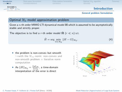
Optimal H2 model approximation problemGiven a n-th order MIMO LTI dynamical model H which is assumed to be asymptoticallystable and strictly proper.
The objective is to find a r-th order model H (r � n) s.t.
H = arg minG∈H2
‖H −G‖H2 . (4)
I the problem is non-convex but smooth↪→with the H∞-norm: non-convex andnon-smooth problem + iterative normcomputation
I As ‖H‖H2 = ‖y‖∞‖u‖2
, a time-domaininterpretation of the error is direct
−4
−3.5
−3
−2.5
−2
−1.5
−1
−0.5
0 05
1015
2025
3035
40
70
75
80
85
90
95
100
Im. partReal part
RelativeH
2error(%
)
C. Poussot-Vassal, P. Vuillemin & I. Pontes Duff [Onera - DCSD] Model Reduction (Approximation) of Large-Scale Systems
Introduction State-space formulation Poles-residues formulation OptimalH2 algorithm Summary
IntroductionGeneral problem formulation
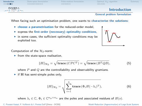
When facing such an optimisation problem, one wants to characterise the solutions:
I choose a parametrisation for the reduced-order model,I express the first-order (necessary) optimality conditions,I in some cases, the sufficient optimality conditions may be
exploited too.
Computation of the H2-norm:I from the state-space realisation,
‖H‖H2 =√
trace (CPCT ) =√
trace (BTQB), (5)
where P and Q are the controllability and observability gramians.I if H has semi-simple poles only,
‖H‖H2 =
√√√√ n∑i=1
trace (ΦiH(−λi)T ), (6)
where λi ∈ C, Φi ∈ Cny×nu are the poles and associated residues of H(s).
C. Poussot-Vassal, P. Vuillemin & I. Pontes Duff [Onera - DCSD] Model Reduction (Approximation) of Large-Scale Systems
Introduction State-space formulation Poles-residues formulation OptimalH2 algorithm Summary
IntroductionGeneral problem formulation
This suggest 2 different parametrisations for H:I the state-space realisation,
H = (A, B, C)I the poles-residues representation.
H(s) =r∑i=1
Φis− λi
=r∑i=1
cibTis− λi
where, if AX = Xdiag(λ1, . . . , λr
),
ci = CXei ∈ Cny , bi =(
eTi X−1B
)T∈ Cnu (7)
↪→assuming H(s) has semi-simple poles only
I they do not ensure stability of H,I both are over-parametrised (the minimal number of parameters is rny + rnu)↪→full state-space realisation: r2 + rnu + rny d.o.f.↪→poles-residues representation: r + rnu + rny d.o.f.
C. Poussot-Vassal, P. Vuillemin & I. Pontes Duff [Onera - DCSD] Model Reduction (Approximation) of Large-Scale Systems
Introduction State-space formulation Poles-residues formulation OptimalH2 algorithm Summary
Outlines
Introduction
First-order optimality conditions: State-space approachProblem statementGradients of the errorLink with the projection framework
First-order optimality conditions: Poles-residues approach
Fixed-point algorithm for optimal H2 reduction
Summary
C. Poussot-Vassal, P. Vuillemin & I. Pontes Duff [Onera - DCSD] Model Reduction (Approximation) of Large-Scale Systems
Introduction State-space formulation Poles-residues formulation OptimalH2 algorithm Summary
First-order optimality conditions: State-space approachProblem statement
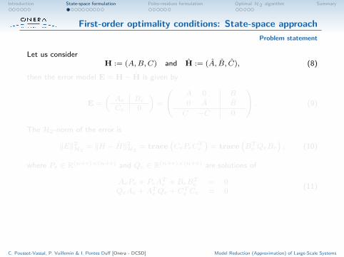
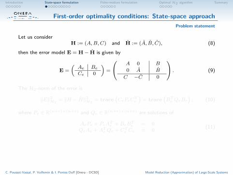
Let us considerH := (A,B,C) and H := (A, B, C), (8)
then the error model E = H− H is given by
E =(Ae BeCe 0
)=
(A 00 A
B
B
C −C 0
). (9)
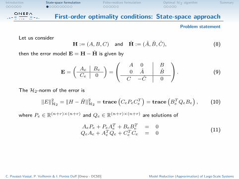
The H2-norm of the error is
‖E‖2H2
= ‖H − H‖2H2
= trace(CePeC
Te
)= trace
(BTe QeBe
), (10)
where Pe ∈ R(n+r)×(n+r) and Qe ∈ R(n+r)×(n+r) are solutions of
AePe + PeATe +BeBTe = 0QeAe +ATe Qe + CTe Ce = 0 (11)
C. Poussot-Vassal, P. Vuillemin & I. Pontes Duff [Onera - DCSD] Model Reduction (Approximation) of Large-Scale Systems
Introduction State-space formulation Poles-residues formulation OptimalH2 algorithm Summary
First-order optimality conditions: State-space approachProblem statement
Let us considerH := (A,B,C) and H := (A, B, C), (8)
then the error model E = H− H is given by
E =(Ae BeCe 0
)=
(A 00 A
B
B
C −C 0
). (9)
The H2-norm of the error is
‖E‖2H2
= ‖H − H‖2H2
= trace(CePeC
Te
)= trace
(BTe QeBe
), (10)
where Pe ∈ R(n+r)×(n+r) and Qe ∈ R(n+r)×(n+r) are solutions of
AePe + PeATe +BeBTe = 0QeAe +ATe Qe + CTe Ce = 0 (11)
C. Poussot-Vassal, P. Vuillemin & I. Pontes Duff [Onera - DCSD] Model Reduction (Approximation) of Large-Scale Systems
Introduction State-space formulation Poles-residues formulation OptimalH2 algorithm Summary
First-order optimality conditions: State-space approachGradients of the error
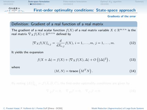
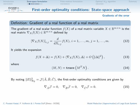
Definition: Gradient of a real function of a real matrixThe gradient of a real scalar function f(X) of a real matrix variable X ∈ Rm×n is thereal matrix ∇Xf(X) ∈ Rm×n defined by
[∇Xf(X)]i,j =d
dXi,jf(X), i = 1, . . . ,m, j = 1, . . . ,m. (12)
It yields the expansion
f(X + ∆) = f(X) + 〈∇Xf(X),∆〉+O(‖∆‖2
), (13)
where〈M,N〉 = trace
(MTN
). (14)
By noting ‖E‖2H2
= J (A, B, C), the first-order optimality conditions are given by
∇AJ = 0, ∇BJ = 0, ∇CJ = 0. (15)
C. Poussot-Vassal, P. Vuillemin & I. Pontes Duff [Onera - DCSD] Model Reduction (Approximation) of Large-Scale Systems
Introduction State-space formulation Poles-residues formulation OptimalH2 algorithm Summary
First-order optimality conditions: State-space approachGradients of the error
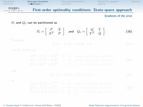
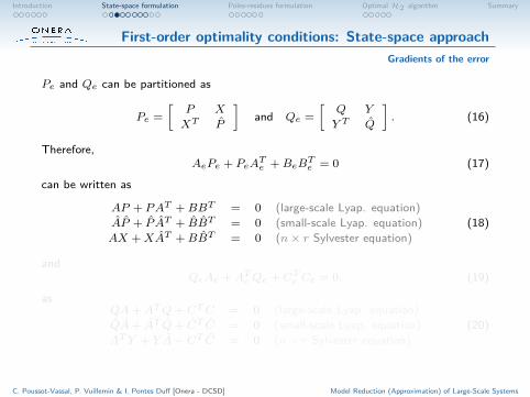
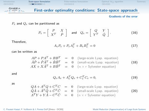
Pe and Qe can be partitioned as
Pe =[
P X
XT P
]and Qe =
[Q Y
Y T Q
]. (16)
Therefore,AePe + PeA
Te +BeB
Te = 0 (17)
can be written as
AP + PAT +BBT = 0 (large-scale Lyap. equation)AP + P AT + BBT = 0 (small-scale Lyap. equation)AX +XAT +BBT = 0 (n× r Sylvester equation)
(18)
andQeAe +ATe Qe + CTe Ce = 0, (19)
asQA+ATQ+ CTC = 0 (large-scale Lyap. equation)QA+ AT Q+ CT C = 0 (small-scale Lyap. equation)ATY + Y A− CT C = 0 (n× r Sylvester equation)
(20)
C. Poussot-Vassal, P. Vuillemin & I. Pontes Duff [Onera - DCSD] Model Reduction (Approximation) of Large-Scale Systems
Introduction State-space formulation Poles-residues formulation OptimalH2 algorithm Summary
First-order optimality conditions: State-space approachGradients of the error
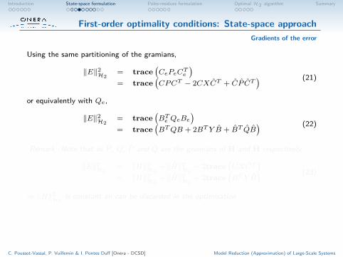
Using the same partitioning of the gramians,
‖E‖2H2
= trace(CePeCTe
)= trace
(CPCT − 2CXCT + CP CT
) (21)
or equivalently with Qe,
‖E‖2H2
= trace(BTe QeBe
)= trace
(BTQB + 2BTY B + BT QB
) (22)
Remark: Note that as P , Q, P and Q are the gramians of H and H respectively,
‖E‖2H2
= ‖H‖2H2
+ ‖H‖2H2− 2trace
(CXCT
)= ‖H‖2
H2+ ‖H‖2
H2+ 2trace
(BTY B
) (23)
⇒ ‖H‖2H2
is constant an can be discarded in the optimisation
C. Poussot-Vassal, P. Vuillemin & I. Pontes Duff [Onera - DCSD] Model Reduction (Approximation) of Large-Scale Systems
Introduction State-space formulation Poles-residues formulation OptimalH2 algorithm Summary
First-order optimality conditions: State-space approachGradients of the error
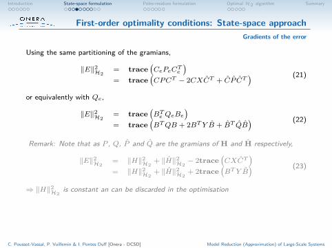
Using the same partitioning of the gramians,
‖E‖2H2
= trace(CePeCTe
)= trace
(CPCT − 2CXCT + CP CT
) (21)
or equivalently with Qe,
‖E‖2H2
= trace(BTe QeBe
)= trace
(BTQB + 2BTY B + BT QB
) (22)
Remark: Note that as P , Q, P and Q are the gramians of H and H respectively,
‖E‖2H2
= ‖H‖2H2
+ ‖H‖2H2− 2trace
(CXCT
)= ‖H‖2
H2+ ‖H‖2
H2+ 2trace
(BTY B
) (23)
⇒ ‖H‖2H2
is constant an can be discarded in the optimisation
C. Poussot-Vassal, P. Vuillemin & I. Pontes Duff [Onera - DCSD] Model Reduction (Approximation) of Large-Scale Systems
Introduction State-space formulation Poles-residues formulation OptimalH2 algorithm Summary
First-order optimality conditions: State-space approachGradients of the error
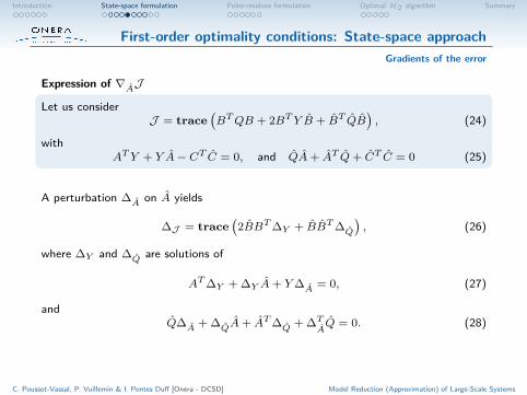
Expression of ∇AJ
Let us considerJ = trace
(BTQB + 2BTY B + BT QB
), (24)
withATY + Y A− CT C = 0, and QA+ AT Q+ CT C = 0 (25)
A perturbation ∆A on A yields
∆J = trace(2BBT∆Y + BBT∆Q
), (26)
where ∆Y and ∆Q are solutions of
AT∆Y + ∆Y A+ Y∆A = 0, (27)
andQ∆A + ∆QA+ AT∆Q + ∆T
AQ = 0. (28)
C. Poussot-Vassal, P. Vuillemin & I. Pontes Duff [Onera - DCSD] Model Reduction (Approximation) of Large-Scale Systems
Introduction State-space formulation Poles-residues formulation OptimalH2 algorithm Summary
First-order optimality conditions: State-space approachGradients of the error
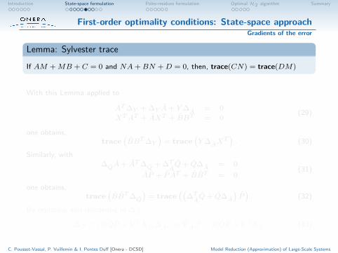
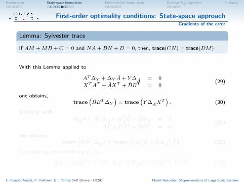
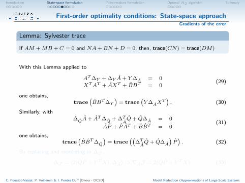
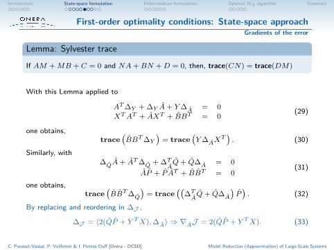
Lemma: Sylvester trace
If AM +MB + C = 0 and NA+BN +D = 0, then, trace(CN) = trace(DM)
With this Lemma applied to
AT∆Y + ∆Y A+ Y∆A = 0XTAT + AXT + BBT = 0
(29)
one obtains,trace
(BBT∆Y
)= trace
(Y∆AX
T). (30)
Similarly, with∆QA+ AT∆Q + ∆T
AQ+ Q∆A = 0
AP + P AT + BBT = 0(31)
one obtains,trace
(BBT∆Q
)= trace
((∆TAQ+ Q∆A
)P). (32)
By replacing and reordering in ∆J ,
∆J = 〈2(QP + Y TX),∆A〉 ⇒ ∇AJ = 2(QP + Y TX). (33)
C. Poussot-Vassal, P. Vuillemin & I. Pontes Duff [Onera - DCSD] Model Reduction (Approximation) of Large-Scale Systems
Introduction State-space formulation Poles-residues formulation OptimalH2 algorithm Summary
First-order optimality conditions: State-space approachGradients of the error
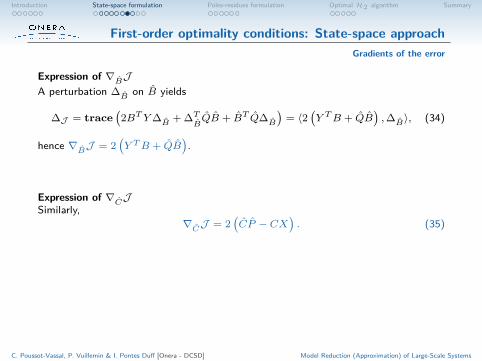
Expression of ∇BJA perturbation ∆B on B yields
∆J = trace(2BTY∆B + ∆T
BQB + BT Q∆B
)= 〈2
(Y TB + QB
),∆B〉, (34)
hence ∇BJ = 2(Y TB + QB
).
Expression of ∇CJSimilarly,
∇CJ = 2(CP − CX
). (35)
C. Poussot-Vassal, P. Vuillemin & I. Pontes Duff [Onera - DCSD] Model Reduction (Approximation) of Large-Scale Systems
Introduction State-space formulation Poles-residues formulation OptimalH2 algorithm Summary
First-order optimality conditions: State-space approachGradients of the error
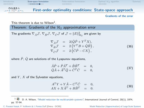
This theorem is due to Wilson1.Theorem: Gradients of the H2 approximation errorThe gradients ∇AJ , ∇BJ , ∇CJ of J = ‖E‖2
H2are given by
∇AJ = 2(QP + Y TX),∇BJ = 2
(Y TB + QB
),
∇CJ = 2(CP − CX
),
(36)
where P , Q are solutions of the Lyapunov equations,
AP + P AT + BBT = 0,QA+ AT Q+ CT C = 0,
(37)
and Y , X of the Sylvester equations,
ATY + Y A− CT C = 0,AX +XAT +BBT = 0.
(38)
1 D. A. Wilson, "Model reduction for multivariable systems", International Journal of Control, 20(1), 1974,pp. 57-64.
C. Poussot-Vassal, P. Vuillemin & I. Pontes Duff [Onera - DCSD] Model Reduction (Approximation) of Large-Scale Systems
Introduction State-space formulation Poles-residues formulation OptimalH2 algorithm Summary
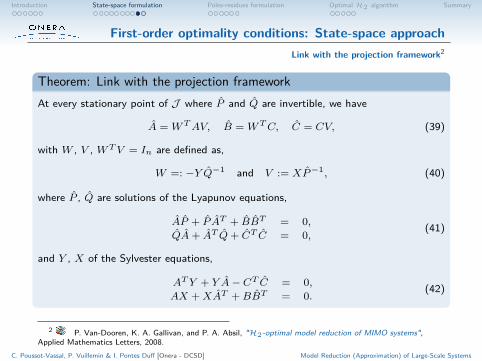
First-order optimality conditions: State-space approachLink with the projection framework2
Theorem: Link with the projection frameworkAt every stationary point of J where P and Q are invertible, we have
A = WTAV, B = WTC, C = CV, (39)
with W , V , WTV = In are defined as,
W =: −Y Q−1 and V := XP−1, (40)
where P , Q are solutions of the Lyapunov equations,
AP + P AT + BBT = 0,QA+ AT Q+ CT C = 0,
(41)
and Y , X of the Sylvester equations,
ATY + Y A− CT C = 0,AX +XAT +BBT = 0.
(42)
2 P. Van-Dooren, K. A. Gallivan, and P. A. Absil, "H2-optimal model reduction of MIMO systems",Applied Mathematics Letters, 2008.
C. Poussot-Vassal, P. Vuillemin & I. Pontes Duff [Onera - DCSD] Model Reduction (Approximation) of Large-Scale Systems
Introduction State-space formulation Poles-residues formulation OptimalH2 algorithm Summary
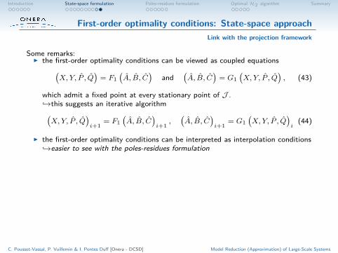
First-order optimality conditions: State-space approachLink with the projection framework
Some remarks:I the first-order optimality conditions can be viewed as coupled equations(
X,Y, P , Q)
= F1(A, B, C
)and
(A, B, C
)= G1
(X,Y, P , Q
), (43)
which admit a fixed point at every stationary point of J .↪→this suggests an iterative algorithm(X,Y, P , Q
)i+1
= F1(A, B, C
)i+1
,(A, B, C
)i+1
= G1(X,Y, P , Q
)i(44)
I the first-order optimality conditions can be interpreted as interpolation conditions↪→easier to see with the poles-residues formulation
C. Poussot-Vassal, P. Vuillemin & I. Pontes Duff [Onera - DCSD] Model Reduction (Approximation) of Large-Scale Systems
Introduction State-space formulation Poles-residues formulation OptimalH2 algorithm Summary
Outlines
Introduction
First-order optimality conditions: State-space approach
First-order optimality conditions: Poles-residues approachProblem statementGradients of the error
Fixed-point algorithm for optimal H2 reduction
Summary
C. Poussot-Vassal, P. Vuillemin & I. Pontes Duff [Onera - DCSD] Model Reduction (Approximation) of Large-Scale Systems
Introduction State-space formulation Poles-residues formulation OptimalH2 algorithm Summary
First-order optimality conditions: Poles-residues approachProblem statement
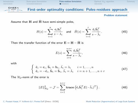
Assume that H and H have semi-simple poles,
H(s) =n∑i=1
cibTis− λi
and H(s) =r∑i=1
cibTis− λi
. (45)
Then the transfer function of the error E = H− H is
E(s) =n+r∑i=1
cibTis− λi
, (46)
with {ci = ci, bi = bi, λi = λi i = 1, . . . , nci = −ci, bi = bi, λi = λi i = n+ 1, . . . , n+ r
(47)
The H2-norm of the error is
‖E‖2H2
= J =n+r∑i=1
trace(
cibTi E(−λi)T). (48)
C. Poussot-Vassal, P. Vuillemin & I. Pontes Duff [Onera - DCSD] Model Reduction (Approximation) of Large-Scale Systems
Introduction State-space formulation Poles-residues formulation OptimalH2 algorithm Summary
First-order optimality conditions: Poles-residues approachGradients of the error
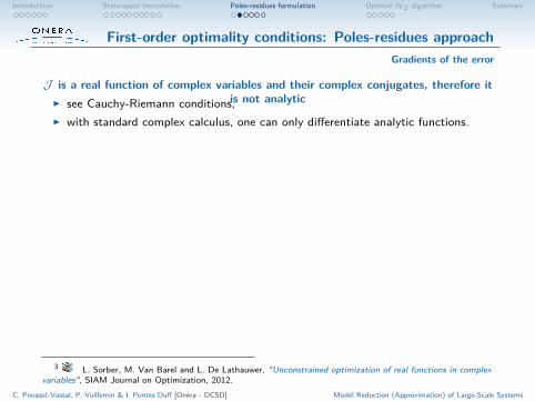
J is a real function of complex variables and their complex conjugates, therefore itis not analyticI see Cauchy-Riemann conditions,
I with standard complex calculus, one can only differentiate analytic functions.
How can we characterise the stationary points of J ?Wirtinger calculusLet f : Cn → R be a real-valued function of a complex vector z (and implicitly itsconjugate) and g : Cn × Cn → R an analytic function with respect to each of itsargument (by treating the other as a constant) such that
f(z) = g(z, z∗), (49)
then the stationary points of f are characterised by
∇zg = 0 or ∇z∗g = 0. (50)
I various implications for optimisation3,I differentiate J by treating conjugate variables as different variables.
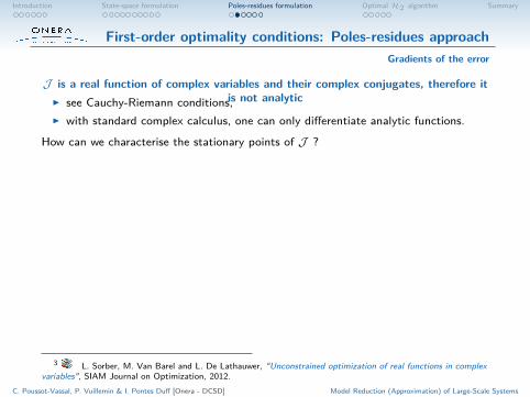
3 L. Sorber, M. Van Barel and L. De Lathauwer, "Unconstrained optimization of real functions in complexvariables", SIAM Journal on Optimization, 2012.
C. Poussot-Vassal, P. Vuillemin & I. Pontes Duff [Onera - DCSD] Model Reduction (Approximation) of Large-Scale Systems
Introduction State-space formulation Poles-residues formulation OptimalH2 algorithm Summary
First-order optimality conditions: Poles-residues approachGradients of the error
J is a real function of complex variables and their complex conjugates, therefore itis not analyticI see Cauchy-Riemann conditions,
I with standard complex calculus, one can only differentiate analytic functions.
How can we characterise the stationary points of J ?
Wirtinger calculusLet f : Cn → R be a real-valued function of a complex vector z (and implicitly itsconjugate) and g : Cn × Cn → R an analytic function with respect to each of itsargument (by treating the other as a constant) such that
f(z) = g(z, z∗), (49)
then the stationary points of f are characterised by
∇zg = 0 or ∇z∗g = 0. (50)
I various implications for optimisation3,I differentiate J by treating conjugate variables as different variables.
3 L. Sorber, M. Van Barel and L. De Lathauwer, "Unconstrained optimization of real functions in complexvariables", SIAM Journal on Optimization, 2012.
C. Poussot-Vassal, P. Vuillemin & I. Pontes Duff [Onera - DCSD] Model Reduction (Approximation) of Large-Scale Systems
Introduction State-space formulation Poles-residues formulation OptimalH2 algorithm Summary
First-order optimality conditions: Poles-residues approachGradients of the error
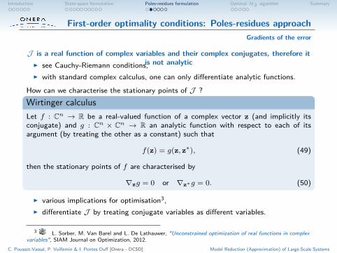
J is a real function of complex variables and their complex conjugates, therefore itis not analyticI see Cauchy-Riemann conditions,
I with standard complex calculus, one can only differentiate analytic functions.
How can we characterise the stationary points of J ?Wirtinger calculusLet f : Cn → R be a real-valued function of a complex vector z (and implicitly itsconjugate) and g : Cn × Cn → R an analytic function with respect to each of itsargument (by treating the other as a constant) such that
f(z) = g(z, z∗), (49)
then the stationary points of f are characterised by
∇zg = 0 or ∇z∗g = 0. (50)
I various implications for optimisation3,I differentiate J by treating conjugate variables as different variables.
3 L. Sorber, M. Van Barel and L. De Lathauwer, "Unconstrained optimization of real functions in complexvariables", SIAM Journal on Optimization, 2012.
C. Poussot-Vassal, P. Vuillemin & I. Pontes Duff [Onera - DCSD] Model Reduction (Approximation) of Large-Scale Systems
Introduction State-space formulation Poles-residues formulation OptimalH2 algorithm Summary
First-order optimality conditions: Poles-residues approachGradients of the error
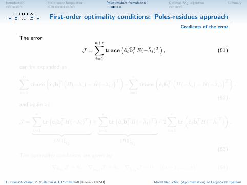
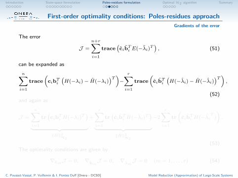
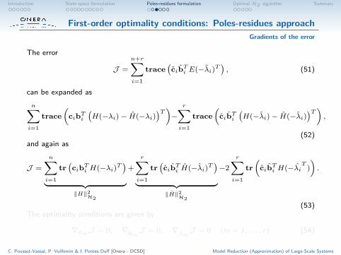
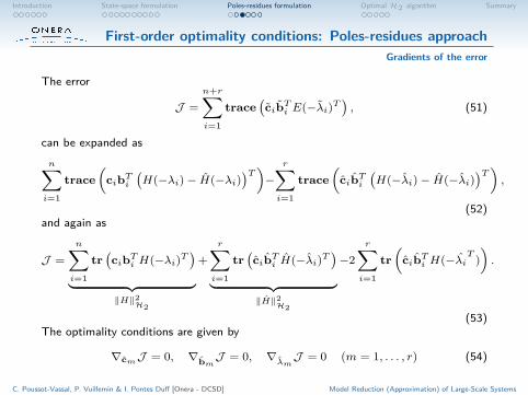
The error
J =n+r∑i=1
trace(
cibTi E(−λi)T), (51)
can be expanded asn∑i=1
trace(
cibTi(H(−λi)− H(−λi)
)T)−
r∑i=1
trace(
cibTi(H(−λi)− H(−λi)
)T),
(52)and again as
J =n∑i=1
tr(
cibTi H(−λi)T)
︸ ︷︷ ︸‖H‖2
H2
+r∑i=1
tr(
cibTi H(−λi)T)
︸ ︷︷ ︸‖H‖2
H2
−2r∑i=1
tr(
cibTi H(−λiT )).
(53)The optimality conditions are given by
∇cmJ = 0, ∇bmJ = 0, ∇λm
J = 0 (m = 1, . . . , r) (54)
C. Poussot-Vassal, P. Vuillemin & I. Pontes Duff [Onera - DCSD] Model Reduction (Approximation) of Large-Scale Systems
Introduction State-space formulation Poles-residues formulation OptimalH2 algorithm Summary
First-order optimality conditions: Poles-residues approachGradients of the error
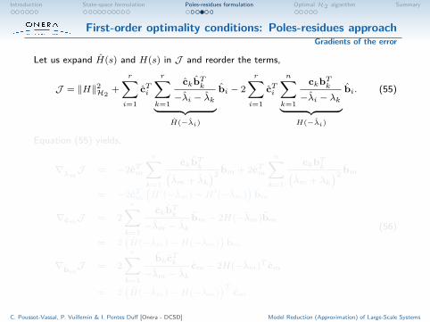
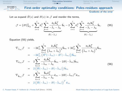
Let us expand H(s) and H(s) in J and reorder the terms,
J = ‖H‖2H2
+r∑i=1
cTi
r∑k=1
ckbTk−λi − λk︸ ︷︷ ︸H(−λi)
bi − 2r∑i=1
cTi
n∑k=1
ckbTk−λi − λk︸ ︷︷ ︸H(−λi)
bi. (55)
Equation (55) yields,
∇λmJ = −2cTm
r∑k=1
ckbTk(λm + λk
)2 bm + 2cTm
n∑k=1
ckbTk(λm + λk
)2 bm
= −2cTm(H′(−λm)−H′(−λm)
)bm
∇cmJ = 2r∑k=1
ckbTk−λm − λk
bm − 2H(−λm)bm
= 2(H(−λm)−H(−λm)
)bm
∇bmJ = 2
r∑k=1
bkcTk−λm − λk
cm − 2H(−λm)T cm
= 2(H(−λm)−H(−λm)
)Tcm
(56)
C. Poussot-Vassal, P. Vuillemin & I. Pontes Duff [Onera - DCSD] Model Reduction (Approximation) of Large-Scale Systems
Introduction State-space formulation Poles-residues formulation OptimalH2 algorithm Summary
First-order optimality conditions: Poles-residues approachGradients of the error
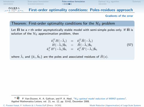
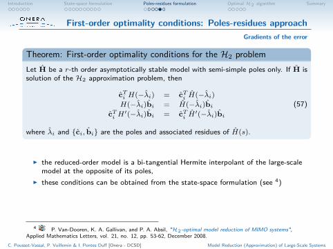
Theorem: First-order optimality conditions for the H2 problemLet H be a r-th order asymptotically stable model with semi-simple poles only. If H issolution of the H2 approximation problem, then
cTi H(−λi) = cTi H(−λi)H(−λi)bi = H(−λi)bi
cTi H′(−λi)bi = cTi H
′(−λi)bi(57)
where λi and {ci, bi} are the poles and associated residues of H(s).
I the reduced-order model is a bi-tangential Hermite interpolant of the large-scalemodel at the opposite of its poles,
I these conditions can be obtained from the state-space formulation (see 4)
4 P. Van-Dooren, K. A. Gallivan, and P. A. Absil, "H2-optimal model reduction of MIMO systems",Applied Mathematics Letters, vol. 21, no. 12, pp. 53-62, December 2008.
C. Poussot-Vassal, P. Vuillemin & I. Pontes Duff [Onera - DCSD] Model Reduction (Approximation) of Large-Scale Systems
Introduction State-space formulation Poles-residues formulation OptimalH2 algorithm Summary
First-order optimality conditions: Poles-residues approachGradients of the error
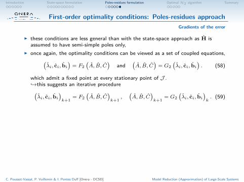
I these conditions are less general than with the state-space approach as H isassumed to have semi-simple poles only,
I once again, the optimality conditions can be viewed as a set of coupled equations,(λi, ci, bi
)= F2
(A, B, C
)and
(A, B, C
)= G2
(λi, ci, bi
). (58)
which admit a fixed point at every stationary point of J .↪→this suggests an iterative procedure(λi, ci, bi
)k+1
= F2(A, B, C
)k+1
,(A, B, C
)k+1
= G2(λi, ci, bi
)k. (59)
C. Poussot-Vassal, P. Vuillemin & I. Pontes Duff [Onera - DCSD] Model Reduction (Approximation) of Large-Scale Systems
Introduction State-space formulation Poles-residues formulation OptimalH2 algorithm Summary
Outlines
Introduction
First-order optimality conditions: State-space approach
First-order optimality conditions: Poles-residues approach
Fixed-point algorithm for optimal H2 reductionIdeaKey elements of the algorithmsIterative Tangential Interpolation Algorithm (ITIA)Example
Summary
C. Poussot-Vassal, P. Vuillemin & I. Pontes Duff [Onera - DCSD] Model Reduction (Approximation) of Large-Scale Systems
Introduction State-space formulation Poles-residues formulation OptimalH2 algorithm Summary
Fixed-point algorithm for optimal H2 reductionIdea
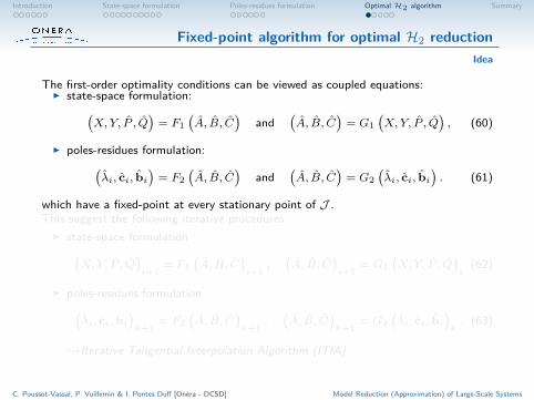
The first-order optimality conditions can be viewed as coupled equations:I state-space formulation:(
X,Y, P , Q)
= F1(A, B, C
)and
(A, B, C
)= G1
(X,Y, P , Q
), (60)
I poles-residues formulation:(λi, ci, bi
)= F2
(A, B, C
)and
(A, B, C
)= G2
(λi, ci, bi
). (61)
which have a fixed-point at every stationary point of J .This suggest the following iterative procedures
I state-space formulation(X,Y, P , Q
)i+1
= F1(A, B, C
)i+1
,(A, B, C
)i+1
= G1(X,Y, P , Q
)i(62)
I poles-residues formulation(λi, ci, bi
)k+1
= F2(A, B, C
)k+1
,(A, B, C
)k+1
= G2(λi, ci, bi
)k. (63)
↪→Iterative Tangential Interpolation Algorithm (ITIA)
C. Poussot-Vassal, P. Vuillemin & I. Pontes Duff [Onera - DCSD] Model Reduction (Approximation) of Large-Scale Systems
Introduction State-space formulation Poles-residues formulation OptimalH2 algorithm Summary
Fixed-point algorithm for optimal H2 reductionIdea
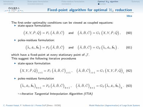
The first-order optimality conditions can be viewed as coupled equations:I state-space formulation:(
X,Y, P , Q)
= F1(A, B, C
)and
(A, B, C
)= G1
(X,Y, P , Q
), (60)
I poles-residues formulation:(λi, ci, bi
)= F2
(A, B, C
)and
(A, B, C
)= G2
(λi, ci, bi
). (61)
which have a fixed-point at every stationary point of J .This suggest the following iterative procedures
I state-space formulation(X,Y, P , Q
)i+1
= F1(A, B, C
)i+1
,(A, B, C
)i+1
= G1(X,Y, P , Q
)i(62)
I poles-residues formulation(λi, ci, bi
)k+1
= F2(A, B, C
)k+1
,(A, B, C
)k+1
= G2(λi, ci, bi
)k. (63)
↪→Iterative Tangential Interpolation Algorithm (ITIA)
C. Poussot-Vassal, P. Vuillemin & I. Pontes Duff [Onera - DCSD] Model Reduction (Approximation) of Large-Scale Systems
Introduction State-space formulation Poles-residues formulation OptimalH2 algorithm Summary
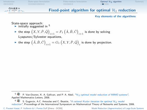
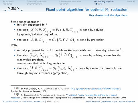
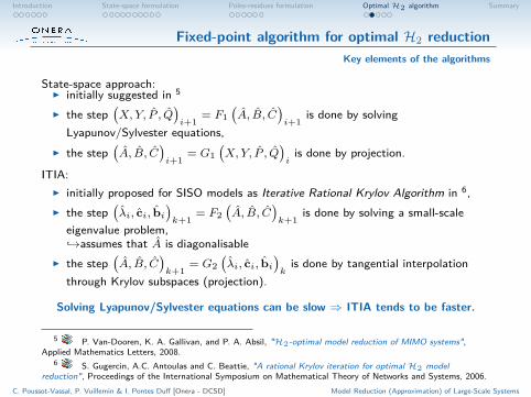
Fixed-point algorithm for optimal H2 reductionKey elements of the algorithms
State-space approach:I initially suggested in 5
I the step(X,Y, P , Q
)i+1
= F1(A, B, C
)i+1
is done by solvingLyapunov/Sylvester equations,
I the step(A, B, C
)i+1
= G1(X,Y, P , Q
)iis done by projection.
ITIA:I initially proposed for SISO models as Iterative Rational Krylov Algorithm in 6,I the step
(λi, ci, bi
)k+1
= F2(A, B, C
)k+1
is done by solving a small-scaleeigenvalue problem,↪→assumes that A is diagonalisable
I the step(A, B, C
)k+1
= G2(λi, ci, bi
)kis done by tangential interpolation
through Krylov subspaces (projection).
Solving Lyapunov/Sylvester equations can be slow ⇒ ITIA tends to be faster.
5 P. Van-Dooren, K. A. Gallivan, and P. A. Absil, "H2-optimal model reduction of MIMO systems",Applied Mathematics Letters, 2008.
6 S. Gugercin, A.C. Antoulas and C. Beattie, "A rational Krylov iteration for optimal H2 modelreduction", Proceedings of the International Symposium on Mathematical Theory of Networks and Systems, 2006.
C. Poussot-Vassal, P. Vuillemin & I. Pontes Duff [Onera - DCSD] Model Reduction (Approximation) of Large-Scale Systems
Introduction State-space formulation Poles-residues formulation OptimalH2 algorithm Summary
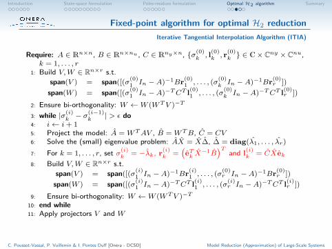
Fixed-point algorithm for optimal H2 reductionIterative Tangential Interpolation Algorithm (ITIA)
Require: A ∈ Rn×n, B ∈ Rn×nu , C ∈ Rny×n, {σ(0)k, l(0)k, r(0)k} ∈ C× Cny × Cnu,
k = 1, . . . , r1: Build V,W ∈ Rn×r s.t.
span(V ) = span([(σ(0)1 In −A)−1Br(0)
1 , . . . , (σ(0)kIn −A)−1Br(0)
r ])span(W ) = span([(σ(0)
1 In −A)−TCT l(0)1 , . . . , (σ(0)
kIn −A)−TCT l(0)
r ])2: Ensure bi-orthogonality: W ←W (WTV )−T
3: while |σ(i)k− σ(i−1)
k| > ε do
4: i← i+ 15: Project the model: A = WTAV , B = WTB, C = CV6: Solve the (small) eigenvalue problem: AX = X∆, ∆ = diag(λ1, . . . , λr)7: For k = 1, . . . , r, set σ(i)
k= −λk, r(i)
k=(
eTk X−1B
)T and l(i)k
= CXek8: Build V,W ∈ Rn×r s.t.
span(V ) = span([(σ(i)1 In −A)−1Br(i)
1 , . . . , (σ(0)r In −A)−1Br(0)
r ])span(W ) = span([(σ(i)
1 In −A)−TCT l(i)1 , . . . , (σ(i)
r In −A)−TCT l(i)r ])
9: Ensure bi-orthogonality: W ←W (WTV )−T10: end while11: Apply projectors V and W
C. Poussot-Vassal, P. Vuillemin & I. Pontes Duff [Onera - DCSD] Model Reduction (Approximation) of Large-Scale Systems
Introduction State-space formulation Poles-residues formulation OptimalH2 algorithm Summary
Fixed-point algorithm for optimal H2 reductionIterative Tangential Interpolation Algorithm (ITIA)
Some remarks,I convergence has been proven only in some specific cases,↪→in practice, it generally converges
I if the algorithm converges, it is not guaranteed to be a local minimum,↪→in practice, the H2-norm of the error generally decreases during the iteration(so its not a maximum) and the resulting reduced-order model are accurate
To summarize,√
leads to a stationary point (generally min.) of the H2 approximation problem,√
numerically very efficient,↪→has been applied to models with more than 700 000 states
√quite simple to implement,
× no control on the approximation error,× stability not always preserved↪→this can be alleviated in exchange for a loss of performance7
7 S. Gugercin, "Iterative SVD-Krylov based method for model reduction of large-scale dynamical systems",CDC, 2005.
C. Poussot-Vassal, P. Vuillemin & I. Pontes Duff [Onera - DCSD] Model Reduction (Approximation) of Large-Scale Systems
Introduction State-space formulation Poles-residues formulation OptimalH2 algorithm Summary
Fixed-point algorithm for optimal H2 reductionExample
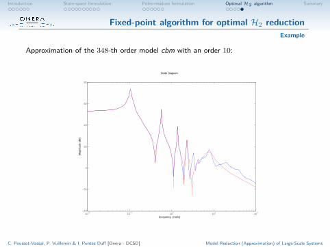
Approximation of the 348-th order model cbm with an order 10:
10−2
10−1
100
101
102
−40
−20
0
20
40
60
80M
agni
tude
(dB
)
Bode Diagram
Frequency (rad/s)
C. Poussot-Vassal, P. Vuillemin & I. Pontes Duff [Onera - DCSD] Model Reduction (Approximation) of Large-Scale Systems

Introduction State-space formulation Poles-residues formulation OptimalH2 algorithm Summary
Outlines
Introduction
First-order optimality conditions: State-space approach
First-order optimality conditions: Poles-residues approach
Fixed-point algorithm for optimal H2 reduction
Summary
C. Poussot-Vassal, P. Vuillemin & I. Pontes Duff [Onera - DCSD] Model Reduction (Approximation) of Large-Scale Systems
Introduction State-space formulation Poles-residues formulation OptimalH2 algorithm Summary
Summary
In this lecture:
I expression of the first-order optimality conditions for the optimal H2 modelreduction problem↪→state-space and poles-residues
I principle of fixed-point algorithms for optimal H2 reduction↪→Iterative Tangential Interpolation Algorithm
Can we have more control on the H2 error throughout iterations?
C. Poussot-Vassal, P. Vuillemin & I. Pontes Duff [Onera - DCSD] Model Reduction (Approximation) of Large-Scale Systems

Introduction State-space formulation Poles-residues formulation OptimalH2 algorithm Summary
Model Reduction (Approximation) of Large-Scale Systems
Optimal H2 approximation: An interpolation point of viewLecture 6
C. Poussot-Vassal, P. Vuillemin & I. Pontes Duff
April 4th-7th, 2016, École Doctorale Systèmes (Toulouse, France)
moremoreΣ
(A,B,C,D)i
Σ
Σ
(A, B, C, D)i
model reduction toolbox
Kr(A,B)
AP + PAT + BBT = 0
WTV
DAE/ODE
State x(t) ∈ Rn, n large orinfinite
Data
ReducedDAE/ODE
Reduced state x(t) ∈ Rrwith r � n(+) Simulation(+) Analysis(+) Control(+) Optimization
Case 1u(f) = [u(f1) . . . u(fi)]y(f) = [y(f1) . . . y(fi)]
Case 2Ex(t) = Ax(t) +Bu(t)y(t) = Cx(t) +Du(t)
Case 3H(s) = e−τs
C. Poussot-Vassal, P. Vuillemin & I. Pontes Duff [Onera - DCSD] Model Reduction (Approximation) of Large-Scale Systems


![Scale Spaces on a Bounded Domainrduits/bdss.pdf · 2013-02-12 · α Scale Spaces on a Bounded Domain 495 parameterized (α ∈ (0,1]) class of scale spaces, the so-called α scale](https://static.fdocument.org/doc/165x107/5f0a8f077e708231d42c39ac/scale-spaces-on-a-bounded-domain-rduitsbdsspdf-2013-02-12-scale-spaces.jpg)


![arXiv:1911.10172v1 [cs.GT] 22 Nov 2019 · through, Cai et al. [12,13,14,15] show that there is a polynomial-time approximation-preserving black-box reduction from multi-dimensional](https://static.fdocument.org/doc/165x107/5f08a02d7e708231d422ef51/arxiv191110172v1-csgt-22-nov-through-cai-et-al-12131415-show-that-there.jpg)