MICROBIAL GROWTH MODELS: A GENERAL … · growth rate (µ max) and the lag phase (λ) are...

Brazilian Journalof ChemicalEngineering

ISSN 0104-6632Printed in Brazil

www.abeq.org.br/bjche

Vol. 34, No. 02, pp. 369 - 375, April - June, 2017dx.doi.org/10.1590/0104-6632.20170342s20150533

*To whom correspondence should be addressed

MICROBIAL GROWTH MODELS: A GENERAL MATHEMATICAL APPROACH TO OBTAIN μmax AND

λ PARAMETERS FROM SIGMOIDAL EMPIRICAL PRIMARY MODELS

D. A. Longhi1*, F. Dalcanton2, G. M. F. de Aragão2, B. A. M. Carciofi2 and J. B. Laurindo2

1Food Engineering, Federal University of Paraná, Jandaia do Sul, PR, Brazil.E-mail: [email protected]

2Department of Chemical and Food Engineering, Federal University of Santa Catarina, Florianópolis, SC, Brazil.

E-mail: [email protected], [email protected], [email protected], [email protected]

(Submitted: August 24, 2015; Revised: December 1, 2015; Accepted: January 14, 2016)

Abstract – Empirical sigmoidal models have been widely applied as primary models to describe microbial growth in foods. In predictive microbiology, the maximum specific growth rate (µmax) and the lag phase (λ) are the parameters of some models and have been considered as biological parameters. The objective of the current study was to propose mathematical equations to obtain the parameters μmax and λ for any sigmoidal empirical growth model. In a case study, the performance was compared of two models based on empirical parameters and two models based on biological parameters. These models were fitted to experimental data for Lactobacillus plantarum in six isothermal conditions. Some advantages of the proposed approach were the practical and biological interpretation of these parameters, and the useful information of the secondary modeling describing the dependence of µmax and λ with the temperature.Keywords: predictive microbiology; mathematical modelling; secondary models; food safety.

INTRODUCTION

In predictive microbiology, the maximum specific growth rate (µmax) and the lag phase (λ) are parameters present in some models and are supposed to have biological meaning (Zwietering et al., 1990). A microbial growth curve is usually expressed as the natural logarithm of the microbial count (y(t) = ln(N)) against time (t). In this curve, the parameter μmax is defined as the slope of the tangent line at the inflection point and the parameter λ is defined as the intercept of this tangent line with the value of the initial microbial count (Pirt, 1975; Zwietering et al., 1990). Both are the main parameters of the mathematical models used to describe microbial growth over time for a single set of environmental conditions, and such models are called

primary models (Whiting and Buchanan, 1993).The temperature is an important variable in food

microbiology, since it varies during the production and distribution chain modifying the microbial growth rate and suitability. In this context, the estimation of the primary model parameters must be done with exactness, for each growth temperature, leading to secondary models that represent well the influence of the temperature on the primary models parameters (Whiting and Buchanan, 1993). The relative errors in the prediction of microbial specific growth rates have been estimated as 20-50% for secondary models and 7-10% for primary models (Masana, 1999). Thus, obtaining great fits for the secondary models can be considered as important as obtaining great fits for primary models.

Brazilian Journal of Chemical Engineering

D. A. Longhi, F. Dalcanton, G. M. F. de Aragão, B. A. M. Carciofi and J. B. Laurindo370

The literature reports a large number of empirical sigmoidal equations that can be applied to describe microbial growth in foods (primary models). Some authors (Tsoularis and Wallace, 2002; Baty and Delignette-Muller, 2004; Peleg and Corradini, 2011; Vázquez et al., 2012; Longhi et al., 2013) have assessed general and specific aspects of some of these models. In general, the mathematical models with biological parameters are interesting because microbiologists can validate them (Baty and Delignette-Muller, 2004).

Zwietering et al. (1990) reparametrized five empirical sigmoidal growth models (Gompertz, Logistic, Richards, Stannard, and Schnute models), generating models with the μmax and λ parameters. Since then, modified Logistic and modified Gompertz models have been used in the reparametrized form (Gospavic et al., 2008; Pal et al., 2008; Slongo et al., 2009; Kreyenschmidt et al., 2010; Longhi et al., 2013). Vázquez et al. (2012) reparametrized two other sigmoidal models (Bertalanffy and Weibull models). However, parameter rearrangements can modify the accuracy of the estimates, making the model fit differ from the original (Zwietering and den Besten, 2011). Therefore, equations transforming one parameter (empirical) to another (with biological meaning) allow comparing different primary models.

The objective of the current study was to propose a generalized mathematical approach to obtain the biological parameters μmax and λ from any sigmoidal empirical equation fitted as a primary model.

THEORETICAL BACKGROUND

Sigmoidal functions frequently applied as primary models to describe microbial growth have one inflection point. The time at the inflection point (tifx) is the root in the Equation (1), and the model response at the inflection point (yifx) is obtained by substituting tifx in the original model equation, as shown in Equation (2).

The maximum specific growth rate (μmax) is obtained by substituting tifx into the first derivative of the sigmoid model, as shown in Equation (3).

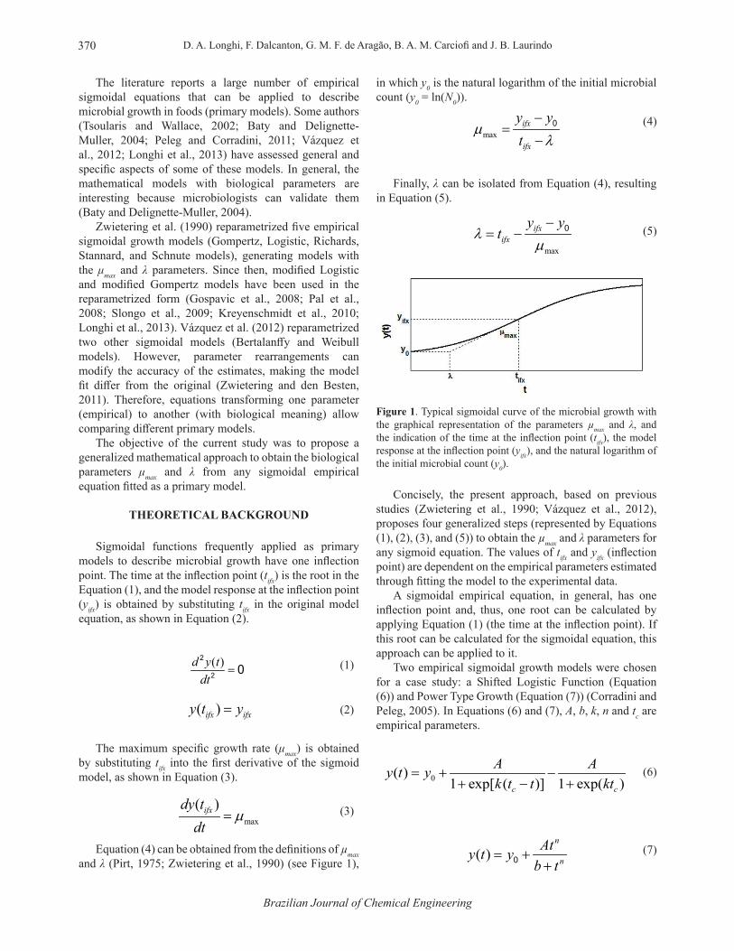
Equation (4) can be obtained from the definitions of µmax and λ (Pirt, 1975; Zwietering et al., 1990) (see Figure 1),

in which y0 is the natural logarithm of the initial microbial count (y0 = ln(N0)).

Finally, λ can be isolated from Equation (4), resulting in Equation (5).

Figure 1. Typical sigmoidal curve of the microbial growth with the graphical representation of the parameters µmax and λ, and the indication of the time at the inflection point (tifx), the model response at the inflection point (yifx), and the natural logarithm of the initial microbial count (y0).

Concisely, the present approach, based on previous studies (Zwietering et al., 1990; Vázquez et al., 2012), proposes four generalized steps (represented by Equations (1), (2), (3), and (5)) to obtain the µmax and λ parameters for any sigmoid equation. The values of tifx and yifx (inflection point) are dependent on the empirical parameters estimated through fitting the model to the experimental data.

A sigmoidal empirical equation, in general, has one inflection point and, thus, one root can be calculated by applying Equation (1) (the time at the inflection point). If this root can be calculated for the sigmoidal equation, this approach can be applied to it.

Two empirical sigmoidal growth models were chosen for a case study: a Shifted Logistic Function (Equation (6)) and Power Type Growth (Equation (7)) (Corradini and Peleg, 2005). In Equations (6) and (7), A, b, k, n and tc are empirical parameters.

( )d y tdt

=2

2 0

( )ifx ifxy t y=

max

( )ifxdy tdt

µ=

maxifx

ifx

y yt

µλ

−=

−0

max

ifxifx

y ytλ

µ−

= − 0

0( )1 exp[ ( )] 1 exp( )c c

A Ay t yk t t kt

= + −+ − +

( )n

n

Aty t yb t

= ++0

(1)

(2)

(3)

(4)

(5)

(6)

(7)

Brazilian Journal of Chemical Engineering Vol 34, No 02, pp. 369 - 375, April - June, 2017

Microbial Growth Models: a General Mathematical Approach to Obtain μmax and λ Parameters from Sigmoidal Empirical Primary Models

371

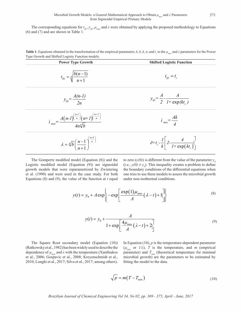
Table 1. Equations obtained in the transformation of the empirical parameters A, b, k, n, and tc to the µmax and λ parameters for the Power Type Growth and Shifted Logistic Function models.

Power Type Growth Shifted Logistic Function

( ) ( )max0

exp 1( ) exp exp 1y t y A t

Aµ

λ = + − − +

( )0

max

( )41 exp 2

Ay t yμ λ tA

= + + − +

The corresponding equations for tifx, yifx, μmax and λ were obtained by applying the proposed methodology to Equations (6) and (7) and are shown in Table 1.

The Gompertz modified model (Equation (8)) and the Logistic modified model (Equation (9)) are sigmoidal growth models that were reparametrized by Zwietering et al. (1990) and were used in the case study. For both Equations (8) and (9), the value of the function at t equal

to zero (y(0)) is different from the value of the parameter y0 (i.e., y(0) ≠ y0). This inequality creates a problem to define the boundary conditions of the differential equations when one tries to use these models to assess the microbial growth under non-isothermal conditions.

(8)

(9)

( 1)1

nifx

b ntn−

=+

ifxA(n-1)y =

2n

( ) ( )n-1 n+1n n

max n

A n-1 n+1ì =

4n b

1

11

nnn nb

nλ

+ − = +

ifx ct t=

expifxc

A Ay = -2 1+ (kt )

maxAkì =4

( )expcc

1 4ë=t - 2-k 1+ kt

The Square Root secondary model (Equation (10)) (Ratkowsky et al., 1982) has been widely used to describe the dependence of µmax and λ with the temperature (Xanthiakos et al., 2006; Gospavic et al., 2008; Kreyenschmidt et al., 2010; Longhi et al., 2017; Silva et al., 2017; among others).

In Equation (10), p is the temperature-dependent parameter (µmax or 1/λ), T is the temperature, and m (empirical parameter) and Tmin (theoretical temperature for minimal microbial growth) are the parameters to be estimated by fitting the model to the data.

( )minp m T T= − (10)



CASE STUDY

Material and methods

Shifted Logistic Function, Power Type Growth, Gompertz Modified, and Logistic Modified primary models were fitted to the growth experimental data of Lactobacillus plantarum in MRS (Man, Rugosa and Sharp) culture medium at six isothermal conditions (4, 8, 12, 16, 20, and 30 °C) (data published by Longhi et al., 2013). The Shifted Logistic Function and Power Type Growth models were fitted in their original forms and the values of the empirical parameters A, b, k, n, and tc were obtained. After that, the biological parameters μmax and λ were obtained by the equations shown in Table 1. Then, the Square Root secondary model (Equation (10)) was fitted to the μmax and λ values, obtained from the Shifted Logistic Function and Power Type Growth models, as dependent on the environmental temperature. The values of μmax and λ for the Gompertz Modified and Logistic Modified models, as well as the fit of the Square Root secondary model, were obtained by Longhi et al. (2013).

The fitting of the mathematical models to the experimental data was performed by the Curve Fitting Tool (cftool) available in the MATLAB R2011b software, version 7.13 (MathWorks, Natick, USA), using a non-linear least squares method and the trust-region reflective Newton algorithm. The value of the initial try of each parameter was selected from the observation of the experimental data. The 95% confidence intervals of the model parameters were obtained in the fitting procedure. The statistical indexes Root-Mean-Square Error (RMSE) and the Adjusted Coefficient of Determination (R2

adj) (standard outputs of the Curve Fitting Tool) were used to assess the ability of the primary and secondary models to describe the experimental data.

Results and discussion

The values of the empirical parameters (A, b, k, n, and tc) and the 95% confidence intervals, estimated by fitting the Power Type Growth and Shifted Logistic Function models to the experimental data, are shown in Table 2. In the same table, the values of µmax and λ obtained for the Power Type Growth and Shifted Logistic Function models with the Equations of Table 1 are shown, as well as the values of µmax and λ from the Gompertz Modified and Logistic Modified models obtained by Longhi et al. (2013).

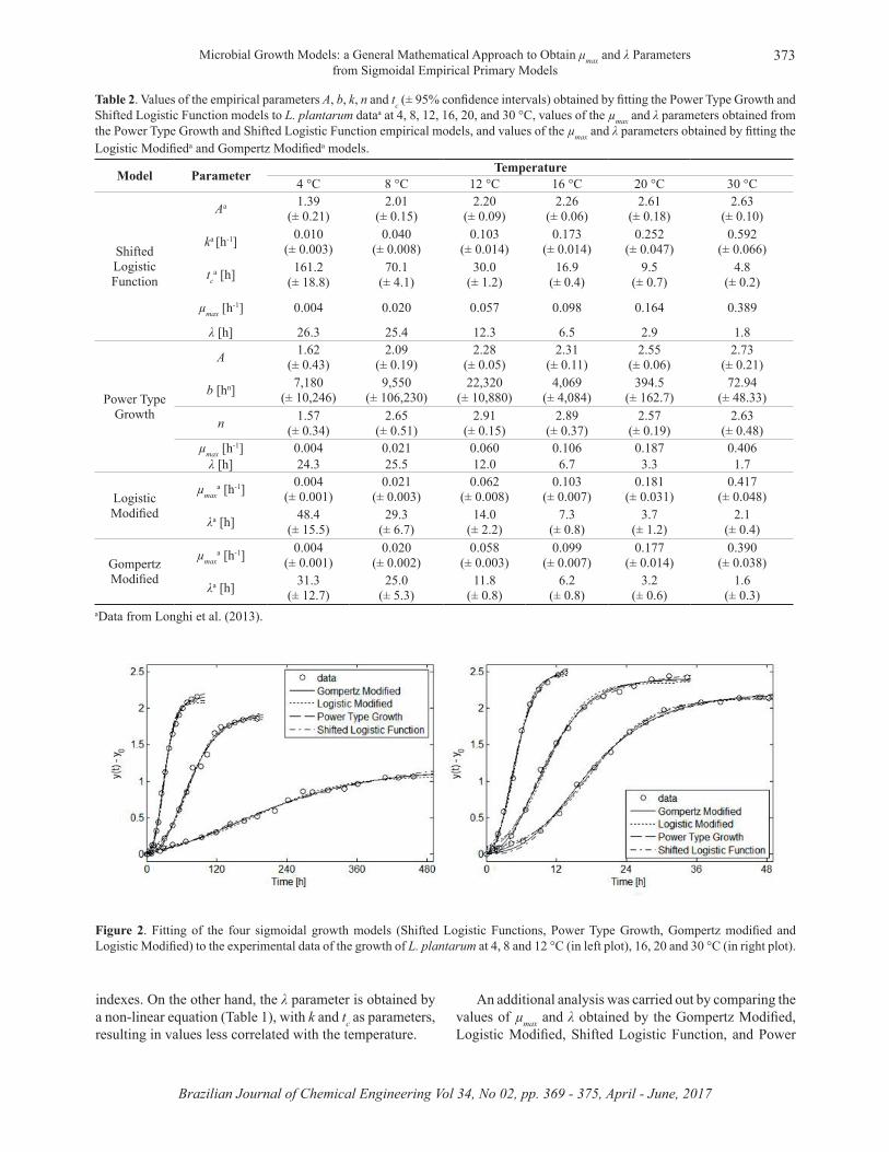
The fitting of the four sigmoidal models (Shifted Logistic Functions, Power Type Growth, Gompertz modified and Logistic Modified) to the experimental data of the growth of L. plantarum at 4, 8, 12, 16, 20 and 30 °C are shown in Figure 2. One important issue to be observed is the availability of experimental data in the stationary growth phase because the parameter related to

the asymptote (the A parameter in the four models) affects the value of the other parameters.

It can be seen in Table 2 that it is difficult to interpret and compare the values of the empirical parameters. On the other hand, the values of the µmax and λ parameters have the same biological meaning and units (µmax [1/h] and λ [h]) for all assessed models (Power Type Growth, Shifted Logistic Function, Logistic Modified and Gompertz Modified), facilitating the interpretation and comparison of these results. Furthermore, the empirical parameters of the Shifted Logistic Function and Power Type Growth models, shown in Table 2, showed larger 95% confidence intervals in relation to µmax and λ for the Gompertz Modified and Logistic Modified models, which can be considered to be another disadvantage of the models built with empirical parameters.

A high uncertainty can be observed for the λ parameter of the sigmoidal models. In general, this uncertainty increases at lower temperatures (as can be seen by the confidence intervals in Table 2) because the distance between the inflection point and the interception with the value of the initial microbial count also increases. At 4 °C, the uncertainty in the value of the λ parameter is greater than 32%, while for the higher temperatures, the uncertainty is lower than 23%.

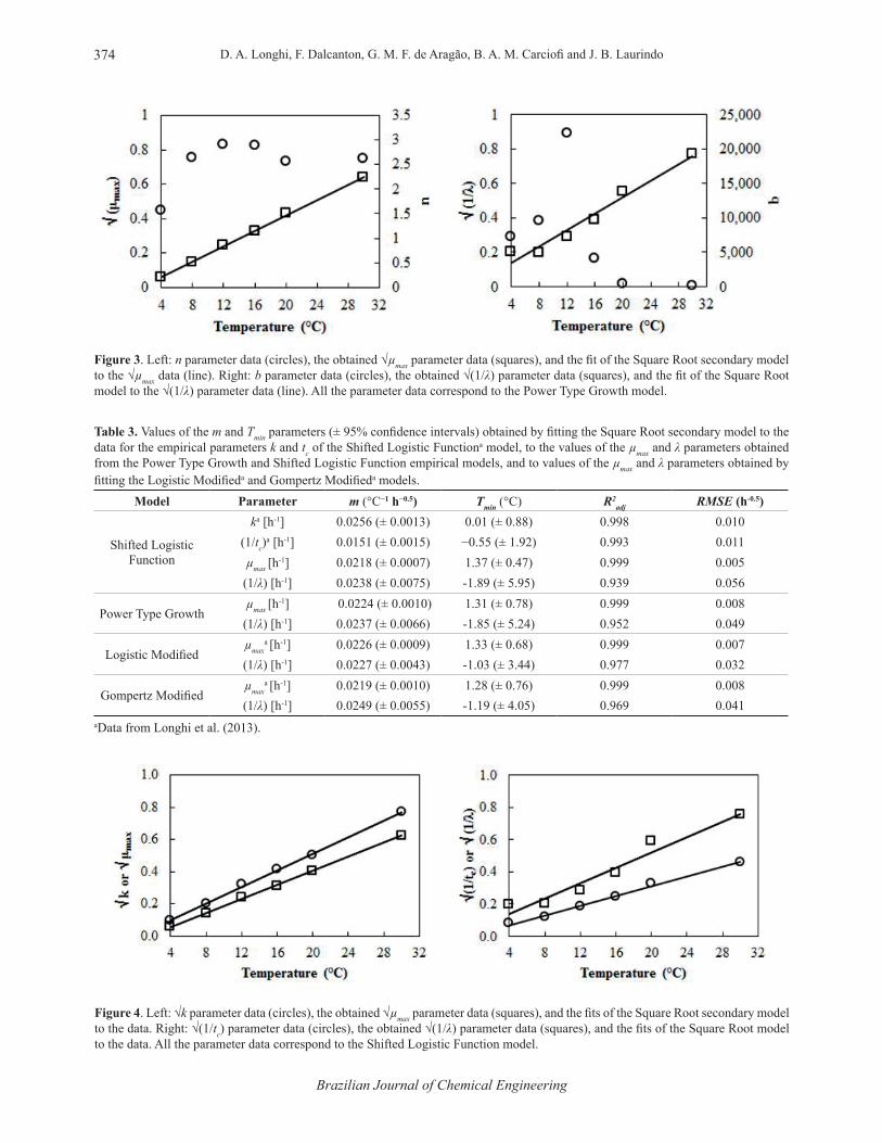
The values of the empirical b and n parameters of the Power Type Growth model and the values of λ and µmax transformed with Equations (1) to (5) are shown in Figure 3 as a function of the temperature. It can be seen that the values of the empirical parameters (b and n) have no clear correlation with the temperature, mainly the b parameter, which presented intermediate values at 4, 8, and 16 °C, a high value at 12 °C, and lower values at 20 and 30 °C. For the n parameter, a rapid increase in their value from 4 to 8 °C can be observed, but from 8 to 30 °C it remains at a conservative value, which even the exponential or power model cannot fit well to the data. Therefore, it becomes difficult to find an appropriate secondary model for these data. On the other hand, the µmax and λ values transformed from the empirical parameters presented clear temperature dependences, which can be described by the Square Root secondary model, resulting in good statistical indexes, as shown in Table 3.

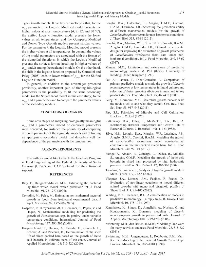
The values of the empirical k and tc parameters of the Shifted Logistic Function model and the values of λ and µmax transformed with Equations (1) to (5) are shown in Figure 4. For the Shifted Logistic Function model, it can be seen that all parameters presented a linear dependence with the temperature, which could be described by the Square Root secondary model, resulting in good statistical indexes, as shown in Table 3. In this case, the statistical indexes of the Square Root secondary model were better for the k and tc empirical parameters than for µmax and λ. As µmax is a linear transformation of k (which is multiplied by (A/4), as shown in Table 1), they have similar statistical



373

Table 2. Values of the empirical parameters A, b, k, n and tc (± 95% confidence intervals) obtained by fitting the Power Type Growth and Shifted Logistic Function models to L. plantarum dataa at 4, 8, 12, 16, 20, and 30 °C, values of the µmax and λ parameters obtained from the Power Type Growth and Shifted Logistic Function empirical models, and values of the µmax and λ parameters obtained by fitting the Logistic Modifieda and Gompertz Modifieda models.

Model Parameter Temperature4 °C 8 °C 12 °C 16 °C 20 °C 30 °C

Shifted Logistic Function

Aa 1.39(± 0.21)

2.01(± 0.15)

2.20(± 0.09)

2.26(± 0.06)

2.61(± 0.18)

2.63(± 0.10)

ka [h-1] 0.010(± 0.003)

0.040(± 0.008)

0.103(± 0.014)

0.173(± 0.014)

0.252(± 0.047)

0.592(± 0.066)

tca [h] 161.2

(± 18.8)70.1

(± 4.1)30.0

(± 1.2)16.9

(± 0.4)9.5

(± 0.7)4.8

(± 0.2)

µmax [h-1] 0.004 0.020 0.057 0.098 0.164 0.389

λ [h] 26.3 25.4 12.3 6.5 2.9 1.8

Power Type Growth

A 1.62(± 0.43)

2.09(± 0.19)

2.28(± 0.05)

2.31(± 0.11)

2.55(± 0.06)

2.73(± 0.21)

b [hn] 7,180(± 10,246)

9,550(± 106,230)

22,320(± 10,880)

4,069(± 4,084)

394.5(± 162.7)

72.94(± 48.33)

n 1.57(± 0.34)

2.65(± 0.51)

2.91(± 0.15)

2.89(± 0.37)

2.57(± 0.19)

2.63(± 0.48)

µmax [h-1] 0.004 0.021 0.060 0.106 0.187 0.406

λ [h] 24.3 25.5 12.0 6.7 3.3 1.7

Logistic Modified

µmaxa [h-1] 0.004

(± 0.001)0.021

(± 0.003)0.062

(± 0.008)0.103

(± 0.007)0.181

(± 0.031)0.417

(± 0.048)

λa [h] 48.4(± 15.5)

29.3(± 6.7)

14.0(± 2.2)

7.3(± 0.8)

3.7(± 1.2)

2.1(± 0.4)

Gompertz Modified

µmaxa [h-1] 0.004

(± 0.001) 0.020

(± 0.002)0.058

(± 0.003)0.099

(± 0.007)0.177

(± 0.014)0.390

(± 0.038)

λa [h] 31.3(± 12.7)

25.0(± 5.3)

11.8(± 0.8)

6.2(± 0.8)

3.2(± 0.6)

1.6(± 0.3)

aData from Longhi et al. (2013).

Figure 2. Fitting of the four sigmoidal growth models (Shifted Logistic Functions, Power Type Growth, Gompertz modified and Logistic Modified) to the experimental data of the growth of L. plantarum at 4, 8 and 12 °C (in left plot), 16, 20 and 30 °C (in right plot).

indexes. On the other hand, the λ parameter is obtained by a non-linear equation (Table 1), with k and tc as parameters, resulting in values less correlated with the temperature.

An additional analysis was carried out by comparing the values of µmax and λ obtained by the Gompertz Modified, Logistic Modified, Shifted Logistic Function, and Power



Figure 3. Left: n parameter data (circles), the obtained √µmax parameter data (squares), and the fit of the Square Root secondary model to the √µmax data (line). Right: b parameter data (circles), the obtained √(1/λ) parameter data (squares), and the fit of the Square Root model to the √(1/λ) parameter data (line). All the parameter data correspond to the Power Type Growth model.

Table 3. Values of the m and Tmin parameters (± 95% confidence intervals) obtained by fitting the Square Root secondary model to the data for the empirical parameters k and tc of the Shifted Logistic Functiona model, to the values of the µmax and λ parameters obtained from the Power Type Growth and Shifted Logistic Function empirical models, and to values of the µmax and λ parameters obtained by fitting the Logistic Modifieda and Gompertz Modifieda models.

Model Parameter m (°C−1 h−0.5) Tmin (°C) R2adj RMSE (h-0.5)

Shifted Logistic Function

ka [h-1] 0.0256 (± 0.0013) 0.01 (± 0.88) 0.998 0.010(1/tc)

a [h-1] 0.0151 (± 0.0015) −0.55 (± 1.92) 0.993 0.011µmax [h

-1] 0.0218 (± 0.0007) 1.37 (± 0.47) 0.999 0.005(1/λ) [h-1] 0.0238 (± 0.0075) -1.89 (± 5.95) 0.939 0.056

Power Type Growthµmax [h

-1] 0.0224 (± 0.0010) 1.31 (± 0.78) 0.999 0.008(1/λ) [h-1] 0.0237 (± 0.0066) -1.85 (± 5.24) 0.952 0.049

Logistic Modifiedµmax

a [h-1] 0.0226 (± 0.0009) 1.33 (± 0.68) 0.999 0.007(1/λ) [h-1] 0.0227 (± 0.0043) -1.03 (± 3.44) 0.977 0.032

Gompertz Modifiedµmax

a [h-1] 0.0219 (± 0.0010) 1.28 (± 0.76) 0.999 0.008(1/λ) [h-1] 0.0249 (± 0.0055) -1.19 (± 4.05) 0.969 0.041

aData from Longhi et al. (2013).

Figure 4. Left: √k parameter data (circles), the obtained √µmax parameter data (squares), and the fits of the Square Root secondary model to the data. Right: √(1/tc) parameter data (circles), the obtained √(1/λ) parameter data (squares), and the fits of the Square Root model to the data. All the parameter data correspond to the Shifted Logistic Function model.



375

Type Growth models. It can be seen in Table 2 that, for the µmax parameter, the Logistic Modified model presents the higher values at most temperatures (4, 8, 12, and 30 °C), the Shifted Logistic Function model presents the lower values at all temperatures, and the Gompertz Modified and Power Type Growth models present similar values. For the parameter λ, the Logistic Modified model presents the higher values at all temperatures. In general, the values of the model parameters are associated with the format of the sigmoidal functions, in which the Logistic Modified presents the strictest format (resulting in higher values of µmax and λ) among the evaluated models. On the other hand, the shift in the logistic function proposed by Corradini and Peleg (2005) leads to lower values of µmax for the Shifted Logistic Function model.

In general, in addition to the advantages presented previously, another important gain of finding biological parameters is the possibility to fit the same secondary model (as the Square Root model in this case study) to the µmax and λ parameters and to compare the parameter values of the secondary models.

CONCLUDING REMARKS

Some advantages of analyzing biologically meaningful µmax and λ parameters instead of empirical parameters were observed, for instance the possibility of comparing different parameter of the sigmoidal models and of finding an appropriate secondary model that describes well the dependence of the parameters with the temperature.

ACKNOWLEDGEMENTS

The authors would like to thank the Graduate Program in Food Engineering of the Federal University of Santa Catarina (UFSC) and CAPES-Brazil for their financial support.

REFERENCES

Baty, F., Delignette-Muller, M.L., Estimating the bacterial lag time: which model, which precision? Int. J. Food Microbiol. 91, 261-277 (2004).

Corradini, M., Peleg, M., Estimating non-isothermal bacterial growth in foods from isothermal experimental data. J Appl. Microbiol. 99, 187-200 (2005).

Gospavic, R., Kreyenschmidt, J., Bruckner, S., Popov, V. and Haque, N., Mathematical modelling for predicting the growth of Pseudomonas spp. in poultry under variable temperature conditions. International Journal of Food Microbiology 127: 290-297 (2008).

Kreyenschmidt, J., Hubner, A., Beierle, E., Chonsch, L., Scherer, A. and Petersen, B., Determination of the shelf life of sliced cooked ham based on the growth of lactic acid bacteria in different steps of the chain. Journal of Applied Microbiology 108: 510-520 (2010).

Longhi, D.A., Dalcanton, F., Aragão, G.M.F., Carciofi, B.A.M., Laurindo, J.B., Assessing the prediction ability of different mathematical models for the growth of Lactobacillus plantarum under non-isothermal conditions. J. Theor. Biol. 335, 88-96 (2013).

Longhi, D.A., Martins, W.F., Silva, N.B., Carciofi, B.A.M., Aragão, G.M.F., Laurindo, J.B., Optimal experimental design for improving the estimation of growth parameters of Lactobacillus viridescens from data under non-isothermal conditions. Int. J. Food Microbiol. 240, 57-62 (2017).

Masana, M.O., Limitations and extensions of predictive microbiology models, M. Phil (thesis), University of Reading, United Kingdom (1999).

Pal, A., Labuza, T., Diez-Gonzalez, F., Comparison of primary predictive models to study the growth of Listeria monocytogenes at low temperatures in liquid cultures and selection of fastest growing ribotypes in meat and turkey product slurries. Food Microbiol. 25, 460-470 (2008).

Peleg, M., Corradini, M.G., Microbial growth curves: what the models tell us and what they cannot. Crit. Rev. Food Sci. Nutr. 51, 917–945 (2011).

Pirt, S.J., Principles of Microbe and Cell Cultivation. Blackwell, Oxford (1975).

Ratkowsky, D.A., Olley, J., McMeekin, T.A., Ball, A. Relationship Between Temperature and Growth Rate of Bacterial Cultures. J. Bacteriol. 149(1), 1-5 (1982).

Silva, N.B., Longhi, D.A., Martins, W.F., Laurindo, J.B., Aragão, G.M.F., Carciofi, B.A.M., Modeling the growth of Lactobacillus viridescens under non-isothermal conditions in vacuum-packed sliced ham. Int. J. Food Microbiol. 240, 97-101 (2017).

Slongo, A., Amauri, R., Camargo, L., Deliza, R., Mathias, S., Aragão, G.M.F., Modeling the growth of lactic acid bacteria in sliced ham processed by high hydrostatic pressure. Lwt-Food Sci. Technol. 42, 303-306 (2009).

Tsoularis, A., Wallace, J., Analysis of logistic growth models. Math. Biosci. 179, 21-55 (2002).

Vázquez, J.A., Lorenzo, J.M., Fuciños, P., Franco, D., Evaluation of non-linear equations to model different animal growths with mono and bisigmoid profiles. J. Theor. Biol. 314, 95–105 (2012).

Whiting, R.C., Buchanan, R.L., A classification of models in predictive microbiology – a reply to K. R. Davey. Food. Microbiol. 10, 175-177 (1993).

Xanthiakos, K., Simos, D., Angelidis, A., Nychas, G. and Koutsoumanis, K., Dynamic modeling of Listeria monocytogenes growth in pasteurized milk. Journal of Applied Microbiology 100: 1289-1298 (2006).

Zwietering, M.H., den Besten, H.M.W., Modelling: One word for many activities and uses. Food Microbiol. 28, 818-822 (2011).

Zwietering, M.H., Jongenburger, I., Rombouts, F.M., Van’t Riet, K., Modeling of the Bacterial Growth Curve. Appl. Environ. Microbiol. 56, 1875-1881 (1990).

MICROBIAL GROWTH MODELS: A GENERAL … · growth rate (µ max) and the lag phase (λ) are...

Documents

Transcript of MICROBIAL GROWTH MODELS: A GENERAL … · growth rate (µ max) and the lag phase (λ) are...