MestRe-C v3 - Από τον πρόεδρο · 4.1 Manual phase correction ... MestRe-C...
135
MestRe-C v3.0
Transcript of MestRe-C v3 - Από τον πρόεδρο · 4.1 Manual phase correction ... MestRe-C...
MestRe-C v3.0

MestRe-C Contents • iii
Contents
Getting Started 1D: A tutorial for beginners. 1 1 Introduction ............................................................................................................................ 1 2 Importing the data set ............................................................................................................. 1 3 Basic graphical manipulation of the FID/Spectrum................................................................ 3
3. 1 How to change the vertical offset of the spectrum on the screen ......................... 3 3.2 How to scroll the spectrum right and left .............................................................. 4 3.3 How to expand (and shrink) selected areas ........................................................... 5 3.4 How to change the appearance of the spectrum: colours, line styles, etc .............. 6
3 Weighting and Fourier Transform .......................................................................................... 7 4 Phase Correction................................................................................................................... 11
4.1 Manual phase correction...................................................................................... 11 4.2 Automatic phase correction ................................................................................. 13
5 Baseline Correction .............................................................................................................. 14 6 Referencing the spectrum ..................................................................................................... 15 7 Integration............................................................................................................................. 16
7.1 Manual Integration .............................................................................................. 16 7.2 Automatic Integration.......................................................................................... 17 7.3 Manipulating the integrals ................................................................................... 17 7.4 Integration manager............................................................................................. 18 7.5 List integrals ........................................................................................................ 18
Quick guide to 2D NMR data processing with MestRe-C 21 1 Introduction .......................................................................................................................... 21 2 Basic steps to process a magnitude 2D spectrum.................................................................. 22 3 Phase Correction................................................................................................................... 25 4 Phase-sensitive 2D spectra.................................................................................................... 25
4.1 Real time 2D phase-correction ............................................................................ 25 5 Baseplane correction............................................................................................................. 29 6 Basic Graphical manipulations. ............................................................................................ 29
Zooming and Scrolling 33 Introduction ............................................................................................................................. 33 Zooming in/out ........................................................................................................................ 33
Zoom-in .......................................................................................................... 33
Manual Zoom .................................................................................................. 34
Expand – Collapse ................................................................................ 35
Zoom-Out ........................................................................................................ 35 Scrolling and Panning.............................................................................................................. 35
iv • Contents Doc-To-Help Standard Template
More Navigation Options... ..................................................................................................... 36
Fourier Transform (FT) and related functions 39 Introduction ............................................................................................................................. 39 FFT and MestRe-C .................................................................................................................. 40
Fourier Transform Dialog.......................................................................................... 40
Window Functions - Apodization 49 Introduction ............................................................................................................................. 49 Exponential multiplication....................................................................................................... 50 Gaussian multiplication ........................................................................................................... 51 Lorentz-to-Gauss for resolution enhancement ......................................................................... 52 Sine bell multiplication............................................................................................................ 53 Sine bell Squared ..................................................................................................................... 54 Hanning function ..................................................................................................................... 54 First point multiplication. ........................................................................................................ 55 TRAF function......................................................................................................................... 55 Trapezoidal .............................................................................................................................. 55 Parabolic multiplication........................................................................................................... 56 Convolution difference ............................................................................................................ 56 Interactive Apodization............................................................................................................ 57
Interactive Weighting in the time domain ................................................................. 57 Interactive Weighting in the frequency domain ........................................................ 58
Phase Correction 61 Introduction ............................................................................................................................. 61 Phase correction of 1D spectra ................................................................................................ 61 Phase correction of 2D spectra ................................................................................................ 63
2D Phase Correction with individual traces .............................................................. 64 Real time 2D phase correction: ................................................................................. 68
Automatic phase correction ..................................................................................................... 68
Baseline/plane Correction 71 Introduction ............................................................................................................................. 71 Polynomial baseline correction................................................................................................ 71 Advanced baseline correction .................................................................................................. 72 Zero-frequency Glitch (Drift Correction): ............................................................................... 74
Integration 77 Introduction ............................................................................................................................. 77 1D Integration.......................................................................................................................... 77
Manual Integration .................................................................................................... 77 Automatic Integration................................................................................................ 79
2D Integration.......................................................................................................................... 80 Calibration of Integrals (Normalization).................................................................................. 80 Integrals list ............................................................................................................................. 81 Integration Manager................................................................................................................. 82 Integral correction.................................................................................................................... 84 Customizing integrals appearance ........................................................................................... 84
Peak Picking 87

MestRe-C Contents • v
Introduction ............................................................................................................................. 87 Semi-Automatic Peak Picking ................................................................................................. 87 Manual Peak Picking (Peak by Peak) ...................................................................................... 88 Peak List .................................................................................................................................. 89
Analysis of arrayed experiments 93 Introduction ............................................................................................................................. 93 Analysis of a DOSY experiment.............................................................................................. 93 Fourier Transform.................................................................................................................... 95 Phase Correction...................................................................................................................... 96 Baseline/plane Correction........................................................................................................ 97 Analysis ................................................................................................................................... 97
Picking points ............................................................................................................ 99
Deconvolution – Line Fitting 105 Introduction ........................................................................................................................... 105 Using the Line Fitting module ............................................................................................... 105 Line fitting options ................................................................................................................ 108
Opening multiple spectra 111 Introduction ........................................................................................................................... 111 Importing multiple spectra.....................................................................................................111
Adding files one-by-one .......................................................................................... 111 Adding a group of files............................................................................................ 114
Automatic processing ............................................................................................................ 116
2D Line approximation: Douglas-Peucker Algorithm 121 Introduction ........................................................................................................................... 121 MestRe-C implementation..................................................................................................... 122
Running MestRe-C from the command line 125 Introduction ........................................................................................................................... 125 Loading an FID/spectrum ...................................................................................................... 125

MestRe-C Getting Started 1D: A tutorial for beginners. • 1
Getting Started 1D: A tutorial for beginners.
1 Introduction This tutorial is designed to help you to become familiar with MestRe-C’s features and capabilities. It is designed to get you quickly into the basics of MestRe-C without an extensive description of every feature. It will show you how to load the data that you have acquired in your spectrometer and the steps you have to follow to get a completed processed spectrum ready to be printed or exported to your favourite word processing program. Bear in mind though, that this tutorial is not intended to show you all the potential of MestRe-C nor we do intend to include an exhaustive survey of NMR data processing techniques
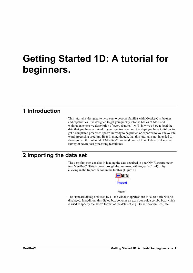
2 Importing the data set The very first step consists in loading the data acquired in your NMR spectrometer into MestRe-C. This is done through the command File/Import (Ctrl–I) or by clicking in the Import button in the toolbar (Figure 1).
Figure 1
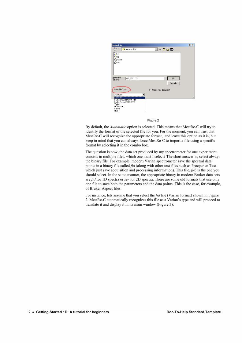
The standard dialog box used by all the window applications to select a file will be displayed. In addition, this dialog box contains an extra control, a combo box, which is used to specify the native format of the data set, e.g. Bruker, Varian, Jeol, etc.
2 • Getting Started 1D: A tutorial for beginners. Doc-To-Help Standard Template
Figure 2
By default, the Automatic option is selected. This means that MestRe-C will try to identify the format of the selected file for you. For the moment, you can trust that MestRe-C will recognize the appropriate format, and leave this option as it is, but keep in mind that you can always force MestRe-C to import a file using a specific format by selecting it in the combo box.
The question is now, the data set produced by my spectrometer for one experiment consists in multiple files: which one must I select? The short answer is, select always the binary file. For example, modern Varian spectrometer save the spectral data points in a binary file called fid (along with other text files such as Procpar or Text which just save acquisition and processing information). This file, fid, is the one you should select. In the same manner, the appropriate binary in modern Bruker data sets are fid for 1D spectra or ser for 2D spectra. There are some old formats that use only one file to save both the parameters and the data points. This is the case, for example, of Bruker Aspect files.
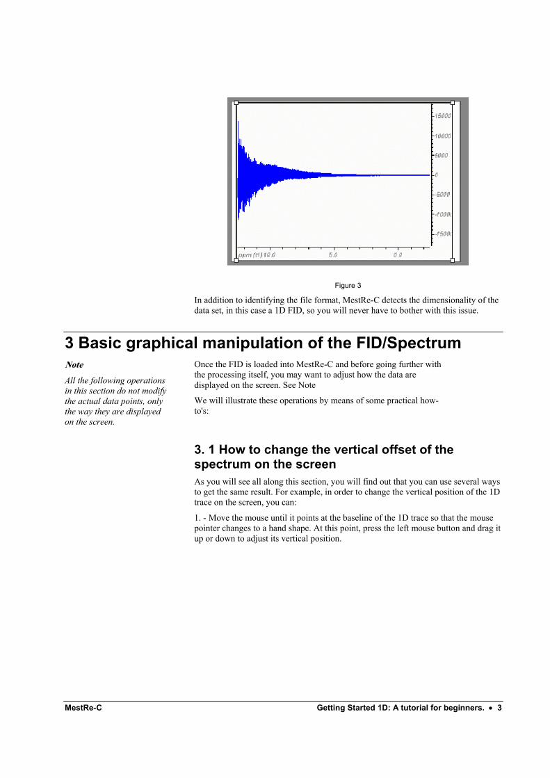
For instance, lets assume that you select the fid file (Varian format) shown in Figure 2. MestRe-C automatically recognizes this file as a Varian’s type and will proceed to translate it and display it in its main window (Figure 3):
MestRe-C Getting Started 1D: A tutorial for beginners. • 3
Figure 3
In addition to identifying the file format, MestRe-C detects the dimensionality of the data set, in this case a 1D FID, so you will never have to bother with this issue.
3 Basic graphical manipulation of the FID/Spectrum Note
All the following operations in this section do not modify the actual data points, only the way they are displayed on the screen.
Once the FID is loaded into MestRe-C and before going further with the processing itself, you may want to adjust how the data are displayed on the screen. See Note
We will illustrate these operations by means of some practical how-to's:
3. 1 How to change the vertical offset of the spectrum on the screen As you will see all along this section, you will find out that you can use several ways to get the same result. For example, in order to change the vertical position of the 1D trace on the screen, you can:
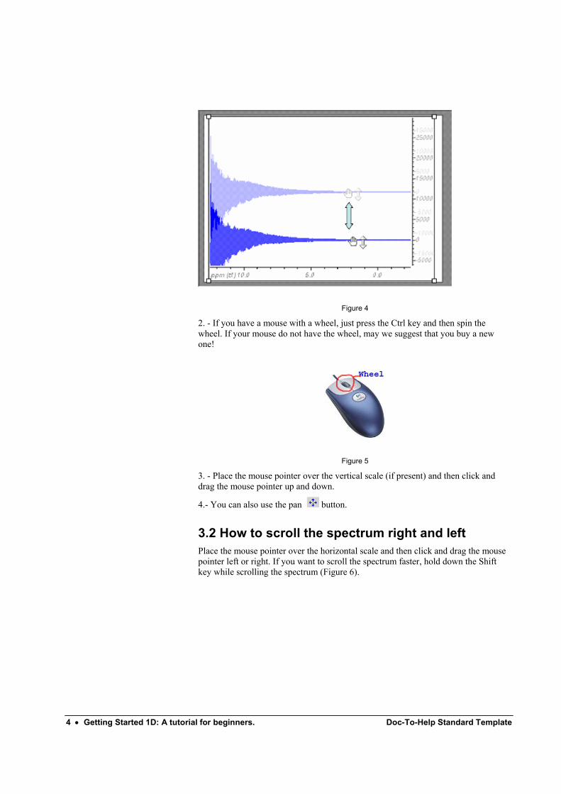
1. - Move the mouse until it points at the baseline of the 1D trace so that the mouse pointer changes to a hand shape. At this point, press the left mouse button and drag it up or down to adjust its vertical position.
4 • Getting Started 1D: A tutorial for beginners. Doc-To-Help Standard Template
Figure 4
2. - If you have a mouse with a wheel, just press the Ctrl key and then spin the wheel. If your mouse do not have the wheel, may we suggest that you buy a new one!
Figure 5
3. - Place the mouse pointer over the vertical scale (if present) and then click and drag the mouse pointer up and down.
4.- You can also use the pan button.
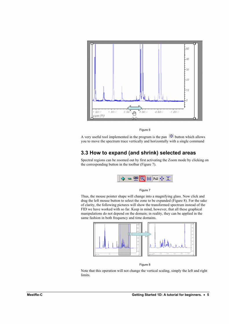
3.2 How to scroll the spectrum right and left Place the mouse pointer over the horizontal scale and then click and drag the mouse pointer left or right. If you want to scroll the spectrum faster, hold down the Shift key while scrolling the spectrum (Figure 6).
MestRe-C Getting Started 1D: A tutorial for beginners. • 5
Figure 6
A very useful tool implemented in the program is the pan button which allows you to move the spectrum trace vertically and horizontally with a single command
3.3 How to expand (and shrink) selected areas Spectral regions can be zoomed out by first activating the Zoom mode by clicking on the corresponding button in the toolbar (Figure 7).
Figure 7
Thus, the mouse pointer shape will change into a magnifying glass. Now click and drag the left mouse button to select the zone to be expanded (Figure 8). For the sake of clarity, the following pictures will show the transformed spectrum instead of the FID we have worked with so far. Keep in mind, however, that all these graphical manipulations do not depend on the domain; in reality, they can be applied in the same fashion in both frequency and time domains.
Figure 8
Note that this operation will not change the vertical scaling, simply the left and right limits.
6 • Getting Started 1D: A tutorial for beginners. Doc-To-Help Standard Template
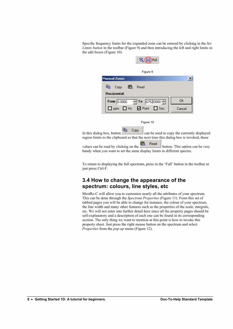
Specific frequency limits for the expanded zone can be entered by clicking in the Set Limits button in the toolbar (Figure 9) and then introducing the left and right limits in the edit boxes (Figure 10).
Figure 9
Figure 10
In this dialog box, button can be used to copy the currently displayed region limits to the clipboard so that the next time this dialog box is invoked, these
values can be read by clicking on the button. This option can be very handy when you want to set the same display limits in different spectra.
To return to displaying the full spectrum, press in the ‘Full’ button in the toolbar or just press Ctrl-F.
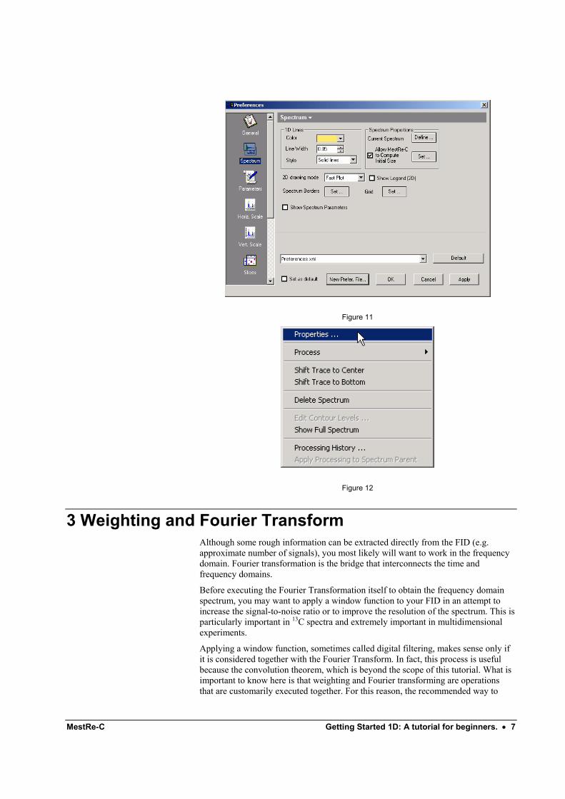
3.4 How to change the appearance of the spectrum: colours, line styles, etc MestRe-C will allow you to customize nearly all the attributes of your spectrum. This can be done through the Spectrum Properties (Figure 11). From this set of tabbed pages you will be able to change for instance, the colour of your spectrum, the line width and many other features such as the properties of the scale, integrals, etc. We will not enter into further detail here since all the property pages should be self-explanatory and a description of each one can be found in its corresponding section. The only thing we want to mention at this point is how to invoke this property sheet. Just press the right mouse button on the spectrum and select Properties from the pop-up menu (Figure 12).
MestRe-C Getting Started 1D: A tutorial for beginners. • 7
Figure 11
Figure 12
3 Weighting and Fourier Transform Although some rough information can be extracted directly from the FID (e.g. approximate number of signals), you most likely will want to work in the frequency domain. Fourier transformation is the bridge that interconnects the time and frequency domains.
Before executing the Fourier Transformation itself to obtain the frequency domain spectrum, you may want to apply a window function to your FID in an attempt to increase the signal-to-noise ratio or to improve the resolution of the spectrum. This is particularly important in 13C spectra and extremely important in multidimensional experiments.
Applying a window function, sometimes called digital filtering, makes sense only if it is considered together with the Fourier Transform. In fact, this process is useful because the convolution theorem, which is beyond the scope of this tutorial. What is important to know here is that weighting and Fourier transforming are operations that are customarily executed together. For this reason, the recommended way to
8 • Getting Started 1D: A tutorial for beginners. Doc-To-Help Standard Template
proceed would be to set the weighting function from within the Fourier Transform dialog box. Typically, you will proceed as follows:
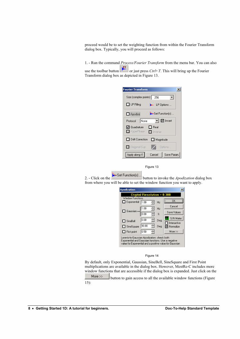
1. - Run the command Process/Fourier Transform from the menu bar. You can also
use the toolbar button or just press Ctrl+T. This will bring up the Fourier Transform dialog box as depicted in Figure 13.
Figure 13
2. - Click on the button to invoke the Apodization dialog box from where you will be able to set the window function you want to apply.
Figure 14
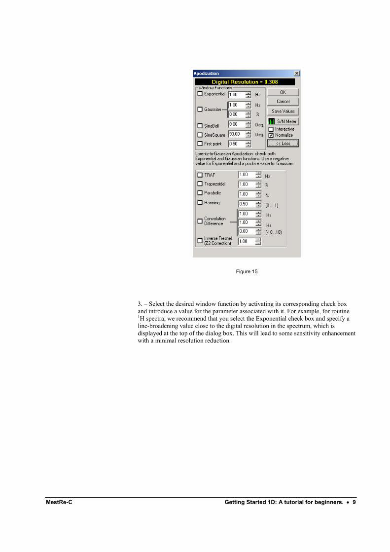
By default, only Exponential, Gaussian, SineBell, SineSquare and First Point multiplications are available in the dialog box. However, MestRe-C includes more window functions that are accessible if the dialog box is expanded. Just click on the
button to gain access to all the available window functions (Figure 15):
MestRe-C Getting Started 1D: A tutorial for beginners. • 9
Figure 15
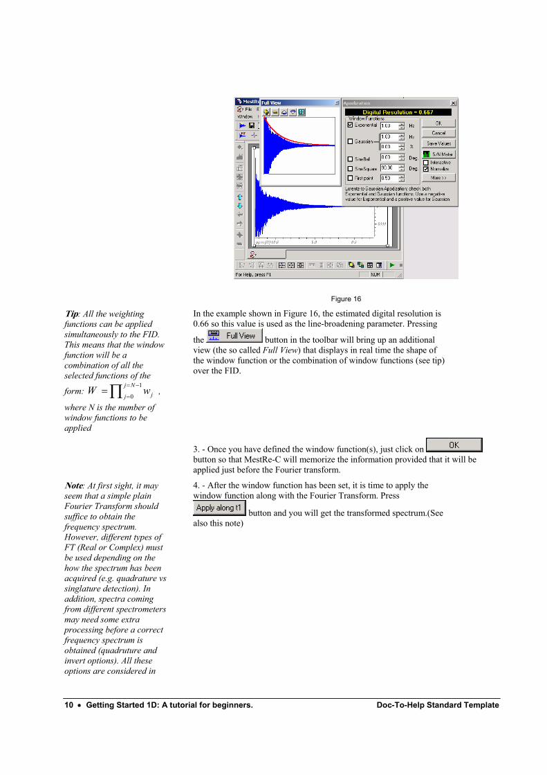
3. – Select the desired window function by activating its corresponding check box and introduce a value for the parameter associated with it. For example, for routine 1H spectra, we recommend that you select the Exponential check box and specify a line-broadening value close to the digital resolution in the spectrum, which is displayed at the top of the dialog box. This will lead to some sensitivity enhancement with a minimal resolution reduction.
10 • Getting Started 1D: A tutorial for beginners. Doc-To-Help Standard Template
Figure 16
Tip: All the weighting functions can be applied simultaneously to the FID. This means that the window function will be a combination of all the selected functions of the
form: ∏ −=
==
1
0
Nj
j jwW ,
where N is the number of window functions to be applied
In the example shown in Figure 16, the estimated digital resolution is 0.66 so this value is used as the line-broadening parameter. Pressing
the button in the toolbar will bring up an additional view (the so called Full View) that displays in real time the shape of the window function or the combination of window functions (see tip) over the FID.
3. - Once you have defined the window function(s), just click on button so that MestRe-C will memorize the information provided that it will be applied just before the Fourier transform.
Note: At first sight, it may seem that a simple plain Fourier Transform should suffice to obtain the frequency spectrum. However, different types of FT (Real or Complex) must be used depending on the how the spectrum has been acquired (e.g. quadrature vs singlature detection). In addition, spectra coming from different spectrometers may need some extra processing before a correct frequency spectrum is obtained (quadruture and invert options). All these options are considered in
4. - After the window function has been set, it is time to apply the window function along with the Fourier Transform. Press
button and you will get the transformed spectrum.(See also this note)
MestRe-C Getting Started 1D: A tutorial for beginners. • 11
the Fourier Transform Dialog Box. If you don’t know how to set all these options, we recommend that you use the default values that MestRe-C will set for you.
Caution: If you follow this scheme, note that when the FT dialog box is called, the apodization check box will be checked. You will have to uncheck it if you don’t want to apodize your spectrum twice!
There is even an alternative way to proceed. You may want to apply the apodization window and see the effect directly on the FID without the Fourier transformation. In order to do this, just select the command Process/Apodize or press Ctrl+W. Now you will get the Apodization dialog box, the same as you got from the FT dialog, but now if you select a window function and press the OK button, the window function will be applied to the FID so you will see how the FID gets modified (Caution).
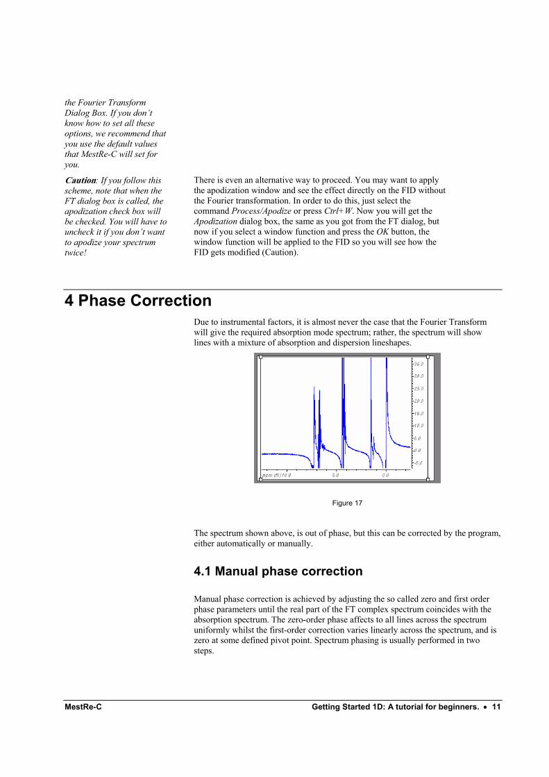
4 Phase Correction Due to instrumental factors, it is almost never the case that the Fourier Transform will give the required absorption mode spectrum; rather, the spectrum will show lines with a mixture of absorption and dispersion lineshapes.
Figure 17
The spectrum shown above, is out of phase, but this can be corrected by the program, either automatically or manually.
4.1 Manual phase correction
Manual phase correction is achieved by adjusting the so called zero and first order phase parameters until the real part of the FT complex spectrum coincides with the absorption spectrum. The zero-order phase affects to all lines across the spectrum uniformly whilst the first-order correction varies linearly across the spectrum, and is zero at some defined pivot point. Spectrum phasing is usually performed in two steps.
12 • Getting Started 1D: A tutorial for beginners. Doc-To-Help Standard Template
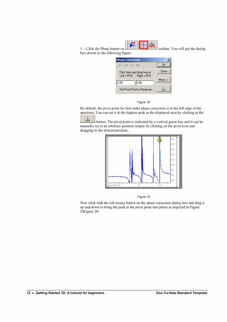
1. - Click the Phase button on toolbar. You will get the dialog box shown in the following figure.
Figure 18
By default, the pivot point for first order phase correction is at the left edge of the spectrum. You can set it to the highest peak in the displayed area by clicking in the
button. The pivot point is indicated by a vertical green line and it can be manually set to an arbitrary position simply by clicking on the pivot icon and dragging to the desired position..
Figure 19
Now click with the left mouse button on the phase correction dialog box and drag it up and down to bring the peak at the pivot point into phase as depicted in Figure 20Figure 20:
MestRe-C Getting Started 1D: A tutorial for beginners. • 13
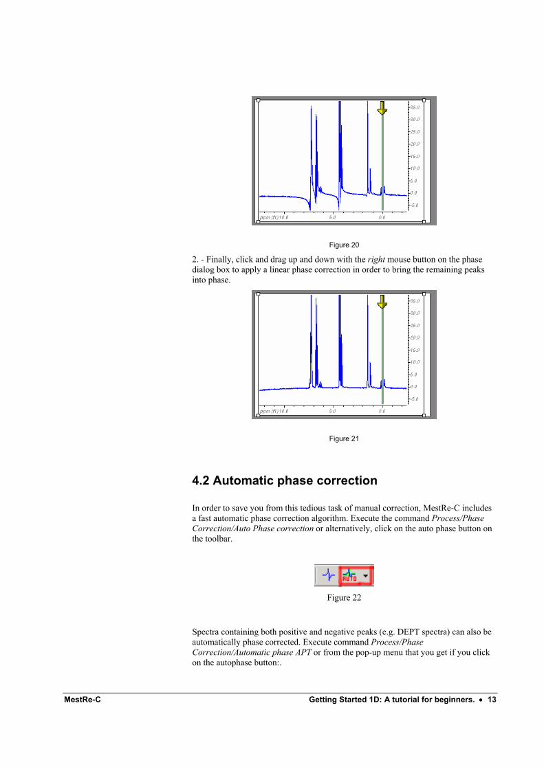
Figure 20
2. - Finally, click and drag up and down with the right mouse button on the phase dialog box to apply a linear phase correction in order to bring the remaining peaks into phase.
Figure 21
4.2 Automatic phase correction
In order to save you from this tedious task of manual correction, MestRe-C includes a fast automatic phase correction algorithm. Execute the command Process/Phase Correction/Auto Phase correction or alternatively, click on the auto phase button on the toolbar.
Figure 22
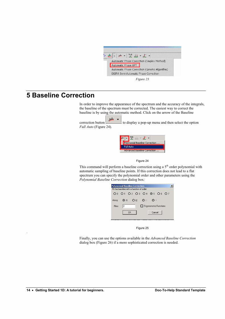
Spectra containing both positive and negative peaks (e.g. DEPT spectra) can also be automatically phase corrected. Execute command Process/Phase Correction/Automatic phase APT or from the pop-up menu that you get if you click on the autophase button:.
14 • Getting Started 1D: A tutorial for beginners. Doc-To-Help Standard Template
Figure 23
5 Baseline Correction In order to improve the appearance of the spectrum and the accuracy of the integrals, the baseline of the spectrum must be corrected. The easiest way to correct the baseline is by using the automatic method. Click on the arrow of the Baseline
correction button to display a pop-up menu and then select the option Full Auto (Figure 24).
Figure 24
This command will perform a baseline correction using a 5th order polynomial with automatic sampling of baseline points. If this correction does not lead to a flat spectrum you can specify the polynomial order and other parameters using the Polynomial Baseline Correction dialog box:
Figure 25 .
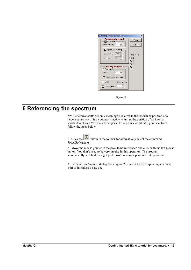
Finally, you can use the options available in the Advanced Baseline Correction dialog box (Figure 26) if a more sophisticated correction is needed.
MestRe-C Getting Started 1D: A tutorial for beginners. • 15
Figure 26
6 Referencing the spectrum NMR chemical shifts are only meaningful relative to the resonance position of a known substance. It is a common practice to assign the position of an internal standard such as TMS or a solvent peak. To reference (calibrate) your spectrum, follow the steps below:
1. Click the button in the toolbar (or alternatively select the command Tools/Reference).
2. Move the mouse pointer to the peak to be referenced and click with the left mouse button. You don’t need to be very precise in this operation. The program automatically will find the right peak position using a parabolic interpolation.
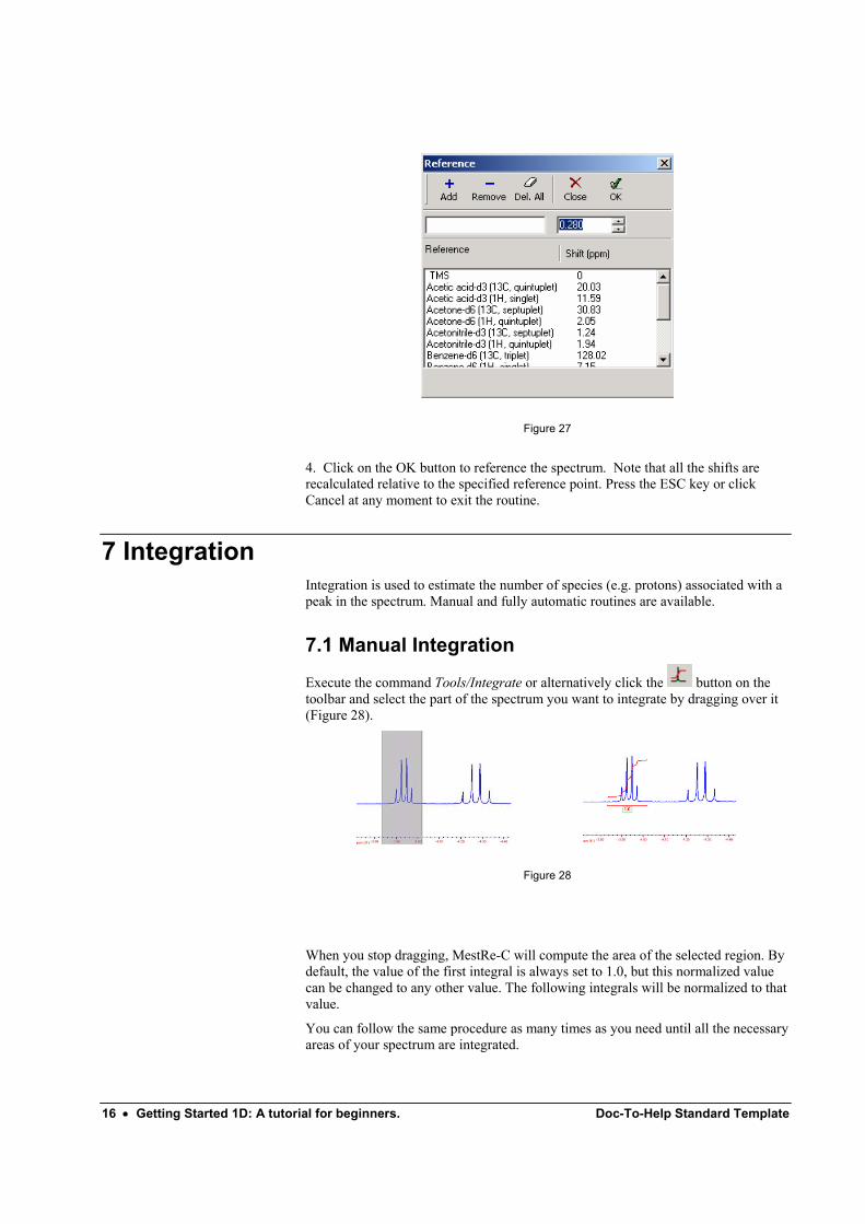
3. In the Solvent Signals dialog box (Figure 27), select the corresponding chemical shift or introduce a new one.
16 • Getting Started 1D: A tutorial for beginners. Doc-To-Help Standard Template
Figure 27
4. Click on the OK button to reference the spectrum. Note that all the shifts are recalculated relative to the specified reference point. Press the ESC key or click Cancel at any moment to exit the routine.
7 Integration Integration is used to estimate the number of species (e.g. protons) associated with a peak in the spectrum. Manual and fully automatic routines are available.
7.1 Manual Integration
Execute the command Tools/Integrate or alternatively click the button on the toolbar and select the part of the spectrum you want to integrate by dragging over it (Figure 28).
Figure 28
When you stop dragging, MestRe-C will compute the area of the selected region. By default, the value of the first integral is always set to 1.0, but this normalized value can be changed to any other value. The following integrals will be normalized to that value.
You can follow the same procedure as many times as you need until all the necessary areas of your spectrum are integrated.
MestRe-C Getting Started 1D: A tutorial for beginners. • 17
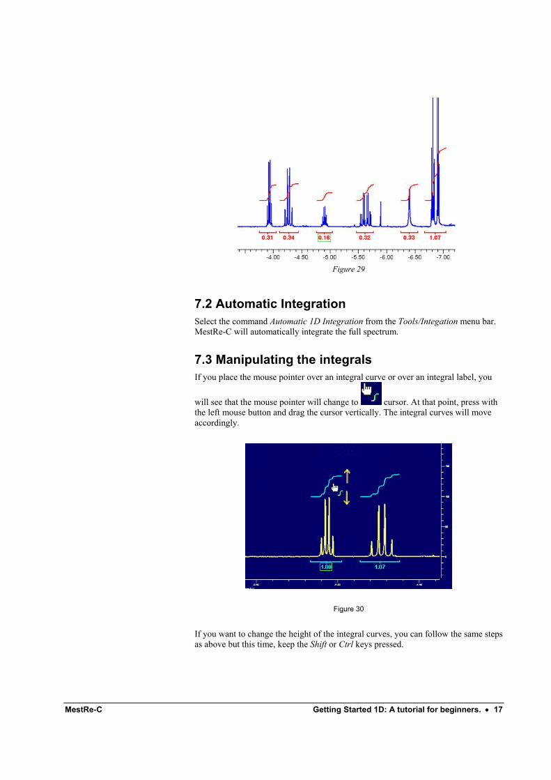
Figure 29
7.2 Automatic Integration Select the command Automatic 1D Integration from the Tools/Integation menu bar. MestRe-C will automatically integrate the full spectrum.
7.3 Manipulating the integrals If you place the mouse pointer over an integral curve or over an integral label, you
will see that the mouse pointer will change to cursor. At that point, press with the left mouse button and drag the cursor vertically. The integral curves will move accordingly.
Figure 30
If you want to change the height of the integral curves, you can follow the same steps as above but this time, keep the Shift or Ctrl keys pressed.
18 • Getting Started 1D: A tutorial for beginners. Doc-To-Help Standard Template
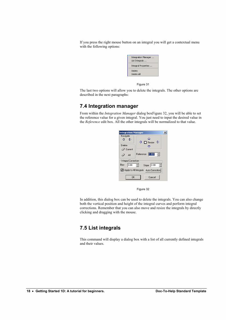
If you press the right mouse button on an integral you will get a contextual menu with the following options:
Figure 31
The last two options will allow you to delete the integrals. The other options are described in the next paragraphs:
7.4 Integration manager From within the Integration Manager dialog boxFigure 32, you will be able to set the reference value for a given integral. You just need to input the desired value in the Reference edit box. All the other integrals will be normalized to that value.
Figure 32
In addition, this dialog box can be used to delete the integrals. You can also change both the vertical position and height of the integral curves and perform integral corrections. Remember that you can also move and resize the integrals by directly clicking and dragging with the mouse.
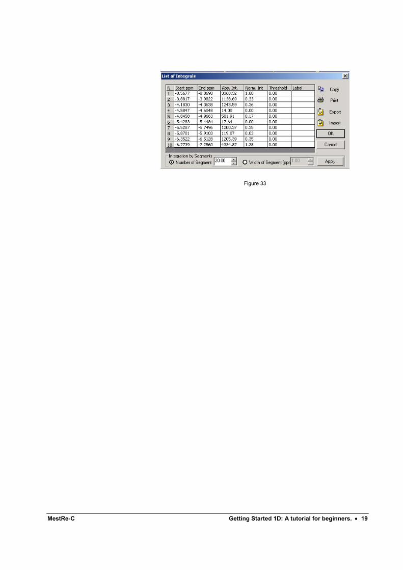
7.5 List integrals
This command will display a dialog box with a list of all currently defined integrals and their values.
MestRe-C Getting Started 1D: A tutorial for beginners. • 19
Figure 33

MestRe-C Quick guide to 2D NMR data processing with MestRe-C • 21
Quick guide to 2D NMR data processing with MestRe-C
1 Introduction
This document will guide you through all the necessary steps to process, display, and print out two-dimensional spectrum sets with MestRe-C. It is assumed that you have read Getting Started: A tutorial for Beginners. By the end of this tutorial you should be able to process magnitude and phase-sensitive 2D NMR spectra.
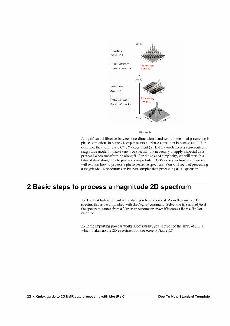
Multidimensional data processing requires only a few new concepts compared to 1D NMR data processing. One important point is that all the processing operations must now be performed along each dimension. For instance, when processing a two-dimensional spectrum you usually follow the flow chart in Figure 34. In MestRe-C, the processing is always started along the acquisition dimension, and finished in the most indirect dimension.
22 • Quick guide to 2D NMR data processing with MestRe-C Doc-To-Help Standard Template
Figure 34
A significant difference between one-dimensional and two-dimensional processing is phase correction. In some 2D experiments no phase correction is needed at all. For example, the useful basic COSY experiment (a 1H-1H correlation) is represented in magnitude mode. In phase sensitive spectra, it is necessary to apply a special data protocol when transforming along f1. For the sake of simplicity, we will start this tutorial describing how to process a magnitude, COSY-type spectrum and then we will explain how to process a phase sensitive spectrum. You will see that processing a magnitude 2D spectrum can be even simpler than processing a 1D spectrum!
2 Basic steps to process a magnitude 2D spectrum
1.- The first task is to read in the data you have acquired. As in the case of 1D spectra, this is accomplished with the Import command. Select the file named fid if the spectrum comes from a Varian spectrometer or ser if it comes from a Bruker machine.
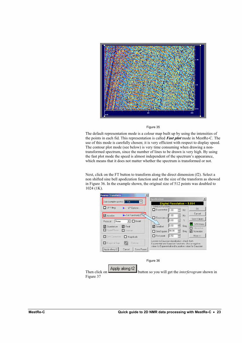
2.- If the importing process works successfully, you should see the array of FIDs which makes up the 2D experiment on the screen (Figure 35)
MestRe-C Quick guide to 2D NMR data processing with MestRe-C • 23
Figure 35
The default representation mode is a colour map built up by using the intensities of the points in each fid. This representation is called Fast plot mode in MestRe-C. The use of this mode is carefully chosen; it is very efficient with respect to display speed. The contour plot mode (see below) is very time consuming when drawing a non-transformed spectrum, since the number of lines to be drawn is very high. By using the fast plot mode the speed is almost independent of the spectrum’s appearance, which means that it does not matter whether the spectrum is transformed or not.
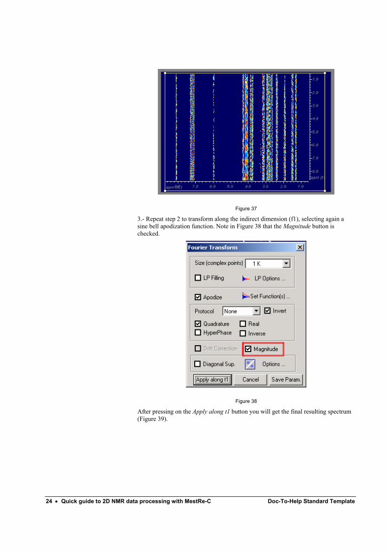
Next, click on the FT button to transform along the direct dimension (f2). Select a non shifted sine bell apodization function and set the size of the transform as showed in Figure 36. In the example shown, the original size of 512 points was doubled to 1024 (1K).
Figure 36
Then click on button so you will get the interferogram shown in Figure 37
24 • Quick guide to 2D NMR data processing with MestRe-C Doc-To-Help Standard Template
Figure 37
3.- Repeat step 2 to transform along the indirect dimension (f1), selecting again a sine bell apodization function. Note in Figure 38 that the Magnitude button is checked.
Figure 38
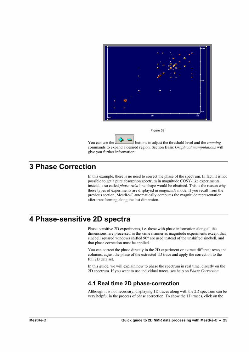
After pressing on the Apply along t1 button you will get the final resulting spectrum (Figure 39).
MestRe-C Quick guide to 2D NMR data processing with MestRe-C • 25
Figure 39
You can use the buttons to adjust the threshold level and the zooming commands to expand a desired region. Section Basic Graphical manipulations will give you further information.
3 Phase Correction In this example, there is no need to correct the phase of the spectrum. In fact, it is not possible to get a pure absorption spectrum in magnitude COSY-like experiments, instead, a so called phase-twist line-shape would be obtained. This is the reason why these types of experiments are displayed in magnitude mode. If you recall from the previous section, MestRe-C automatically computes the magnitude representation after transforming along the last dimension.
4 Phase-sensitive 2D spectra Phase-sensitive 2D experiments, i.e. those with phase information along all the dimensions, are processed in the same manner as magnitude experiments except that sinebell squared windows shifted 90° are used instead of the unshifted sinebell, and that phase correction must be applied.
You can correct the phase directly in the 2D experiment or extract different rows and columns, adjust the phase of the extracted 1D trace and apply the correction to the full 2D data set.
In this guide, we will explain how to phase the spectrum in real time, directly on the 2D spectrum. If you want to use individual traces, see help on Phase Correction.
4.1 Real time 2D phase-correction Although it is not necessary, displaying 1D traces along with the 2D spectrum can be very helpful in the process of phase correction. To show the 1D traces, click on the
26 • Quick guide to 2D NMR data processing with MestRe-C Doc-To-Help Standard Template
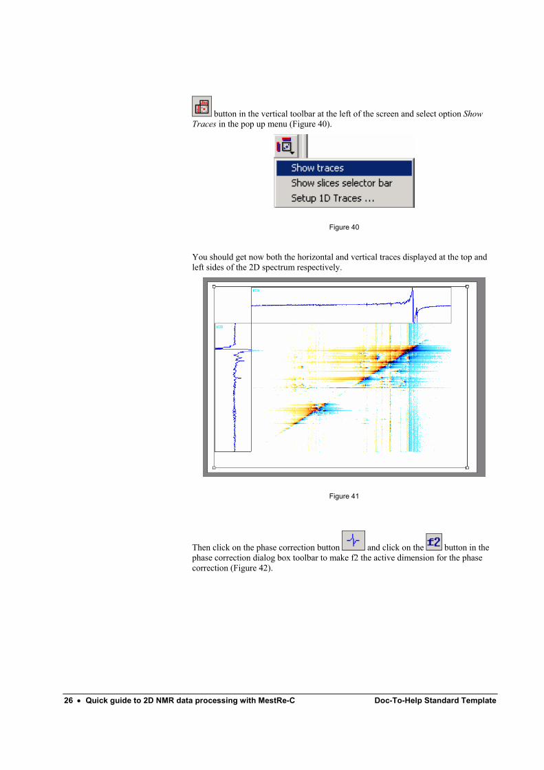
button in the vertical toolbar at the left of the screen and select option Show Traces in the pop up menu (Figure 40).
Figure 40
You should get now both the horizontal and vertical traces displayed at the top and left sides of the 2D spectrum respectively.
Figure 41
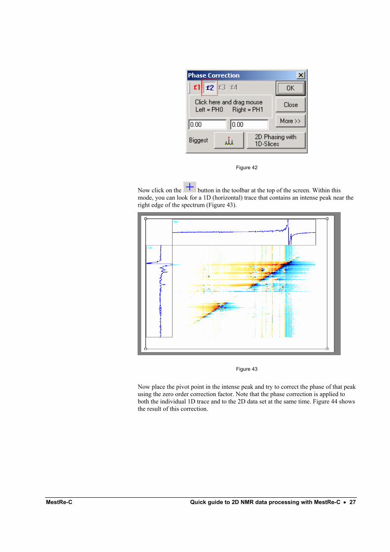
Then click on the phase correction button and click on the button in the phase correction dialog box toolbar to make f2 the active dimension for the phase correction (Figure 42).
MestRe-C Quick guide to 2D NMR data processing with MestRe-C • 27
Figure 42
Now click on the button in the toolbar at the top of the screen. Within this mode, you can look for a 1D (horizontal) trace that contains an intense peak near the right edge of the spectrum (Figure 43).
Figure 43
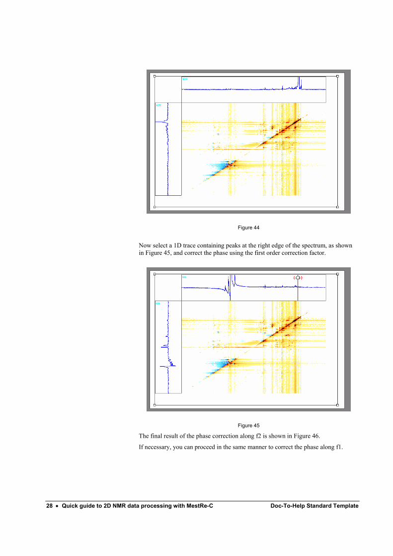
Now place the pivot point in the intense peak and try to correct the phase of that peak using the zero order correction factor. Note that the phase correction is applied to both the individual 1D trace and to the 2D data set at the same time. Figure 44 shows the result of this correction.
28 • Quick guide to 2D NMR data processing with MestRe-C Doc-To-Help Standard Template
Figure 44
Now select a 1D trace containing peaks at the right edge of the spectrum, as shown in Figure 45, and correct the phase using the first order correction factor.
Figure 45
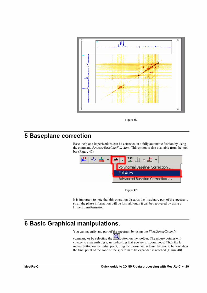
The final result of the phase correction along f2 is shown in Figure 46.
If necessary, you can proceed in the same manner to correct the phase along f1.
MestRe-C Quick guide to 2D NMR data processing with MestRe-C • 29
Figure 46
5 Baseplane correction Baseline/plane imperfections can be corrected in a fully automatic fashion by using the command Process/Baseline/Full Auto. This option is also available from the tool bar (Figure 47):
Figure 47
It is important to note that this operation discards the imaginary part of the spectrum, so all the phase information will be lost, although it can be recovered by using a Hilbert transformation.
6 Basic Graphical manipulations. You can magnify any part of the spectrum by using the View/Zoom/Zoom In
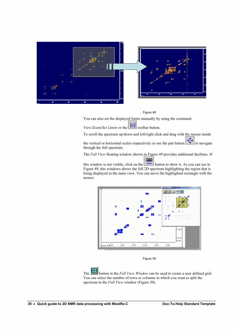
command or by selecting the button on the toolbar. The mouse pointer will change to a magnifying glass indicating that you are in zoom mode. Click the left mouse button on the initial point, drag the mouse and release the mouse button when the final point of the zone of the spectrum to be expanded is reached (Figure 48).
30 • Quick guide to 2D NMR data processing with MestRe-C Doc-To-Help Standard Template
Figure 48
You can also set the displayed limits manually by using the command
View/Zoom/Set Limits or the toolbar button.
To scroll the spectrum up/down and left/right click and drag with the mouse inside
the vertical or horizontal scales respectively or use the pan button to navigate through the full spectrum.
The Full View floating window shown in Figure 49 provides additional facilities. If
this window is not visible, click on the button to show it. As you can see in Figure 49, this windows shows the full 2D spectrum highlighting the region that is being displayed in the main view. You can move the highlighted rectangle with the mouse.
Figure 49
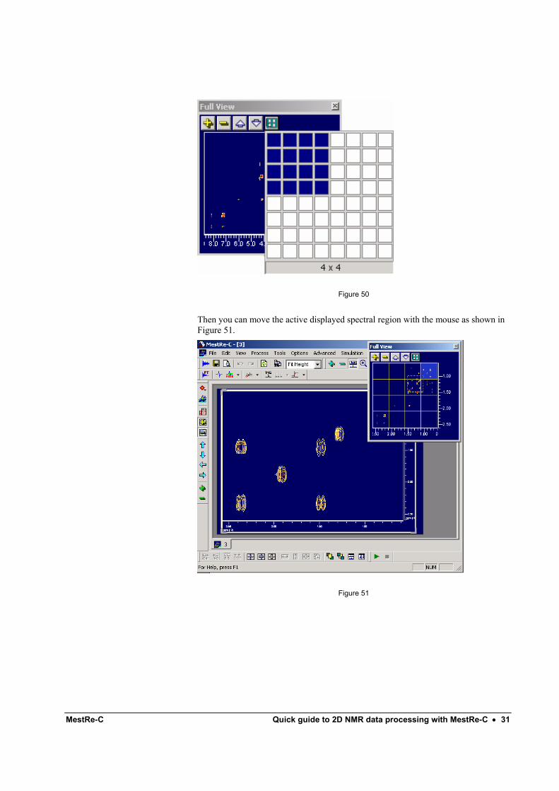
The button in the Full View Window can be used to create a user defined grid. You can select the number of rows or columns in which you want to split the spectrum in the Full View window (Figure 50).
MestRe-C Quick guide to 2D NMR data processing with MestRe-C • 31
Figure 50
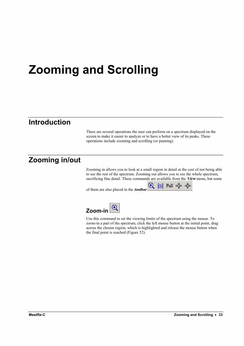
Then you can move the active displayed spectral region with the mouse as shown in Figure 51.
Figure 51

MestRe-C Zooming and Scrolling • 33
Zooming and Scrolling
Introduction There are several operations the user can perform on a spectrum displayed on the screen to make it easier to analyze or to have a better view of its peaks. These operations include zooming and scrolling (or panning).
Zooming in/out Zooming in allows you to look at a small region in detail at the cost of not being able to see the rest of the spectrum. Zooming out allows you to see the whole spectrum, sacrificing fine detail. These commands are available from the View menu, but some
of them are also placed in the toolbar
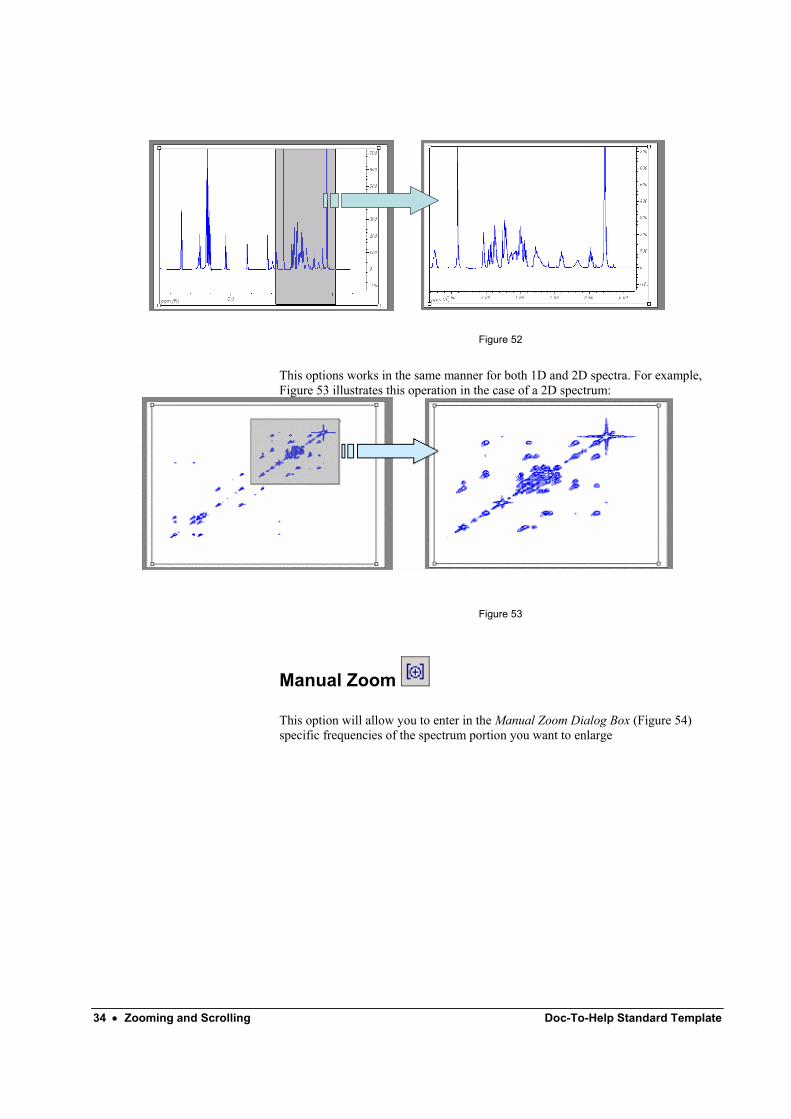
Zoom-in Use this command to set the viewing limits of the spectrum using the mouse. To zoom-in a part of the spectrum, click the left mouse button at the initial point, drag across the chosen region, which is highlighted and release the mouse button when the final point is reached (Figure 52).
34 • Zooming and Scrolling Doc-To-Help Standard Template
Figure 52
This options works in the same manner for both 1D and 2D spectra. For example, Figure 53 illustrates this operation in the case of a 2D spectrum:
Figure 53
Manual Zoom
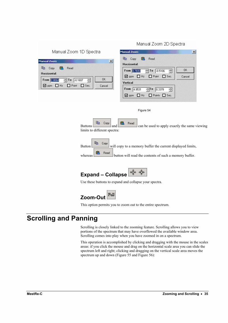
This option will allow you to enter in the Manual Zoom Dialog Box (Figure 54) specific frequencies of the spectrum portion you want to enlarge
MestRe-C Zooming and Scrolling • 35
Figure 54
Buttons and can be used to apply exactly the same viewing limits to different spectra:
Button will copy to a memory buffer the current displayed limits,
whereas button will read the contents of such a memory buffer.
Expand – Collapse Use these buttons to expand and collapse your spectra.
Zoom-Out This option permits you to zoom out to the entire spectrum.
Scrolling and Panning Scrolling is closely linked to the zooming feature. Scrolling allows you to view portions of the spectrum that may have overflowed the available window area. Scrolling comes into play when you have zoomed in on a spectrum.
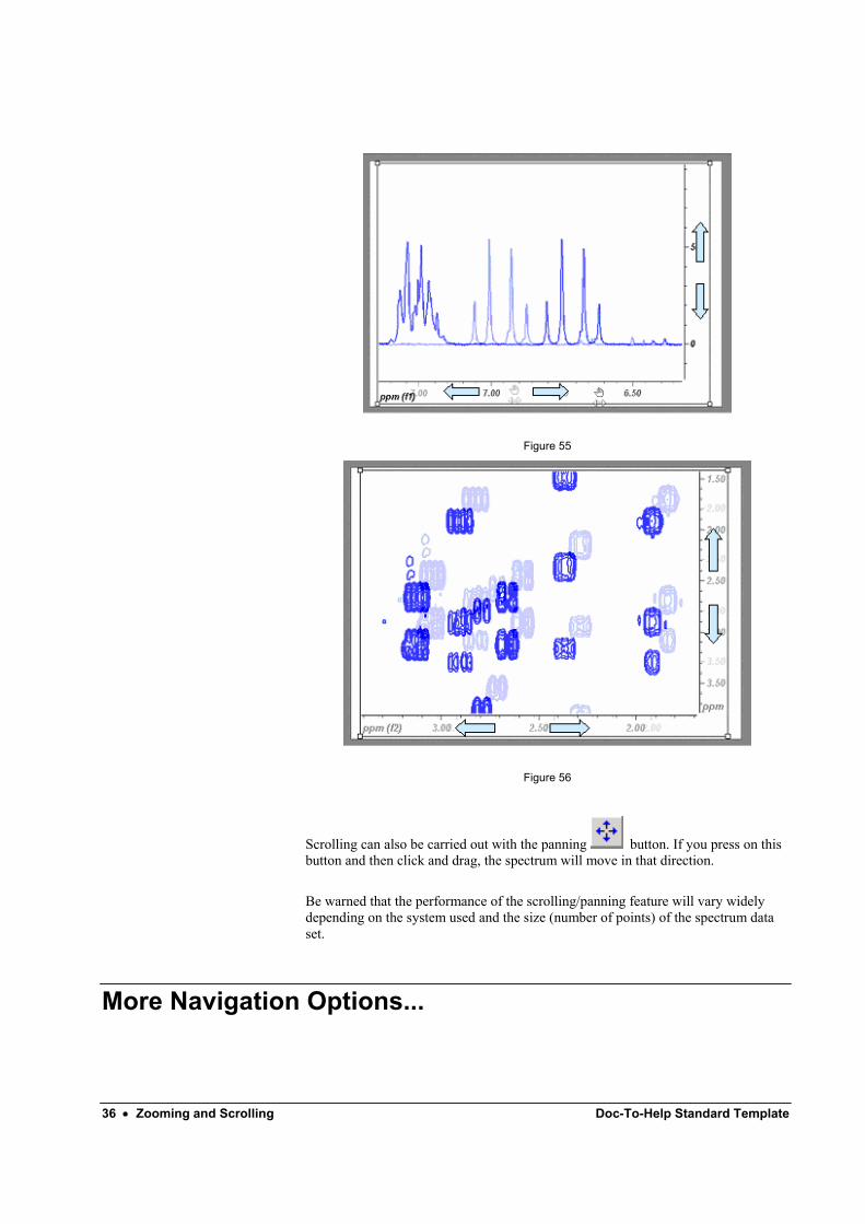
This operation is accomplished by clicking and dragging with the mouse in the scales areas: if you click the mouse and drag on the horizontal scale area you can slide the spectrum left and right; clicking and dragging on the vertical scale area moves the spectrum up and down (Figure 55 and Figure 56):
36 • Zooming and Scrolling Doc-To-Help Standard Template
Figure 55
Figure 56
Scrolling can also be carried out with the panning button. If you press on this button and then click and drag, the spectrum will move in that direction.
Be warned that the performance of the scrolling/panning feature will vary widely depending on the system used and the size (number of points) of the spectrum data set.
More Navigation Options...
MestRe-C Zooming and Scrolling • 37
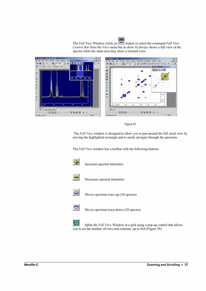
The Full View Window (click on button or select the command Full View Control Bar from the View menu bar to show it) always shows a full view of the spectra while the main area may show a zoomed view.
Figure 57
The Full View window is designed to allow you to pan around the full sized view by moving the highlighted rectangle and to easily navigate through the spectrum.
The Full View window has a toolbar with the following buttons:
Increases spectral intensities
Decreases spectral intensities
Moves spectrum trace up (1D spectra)
Moves spectrum trace down (1D spectra)
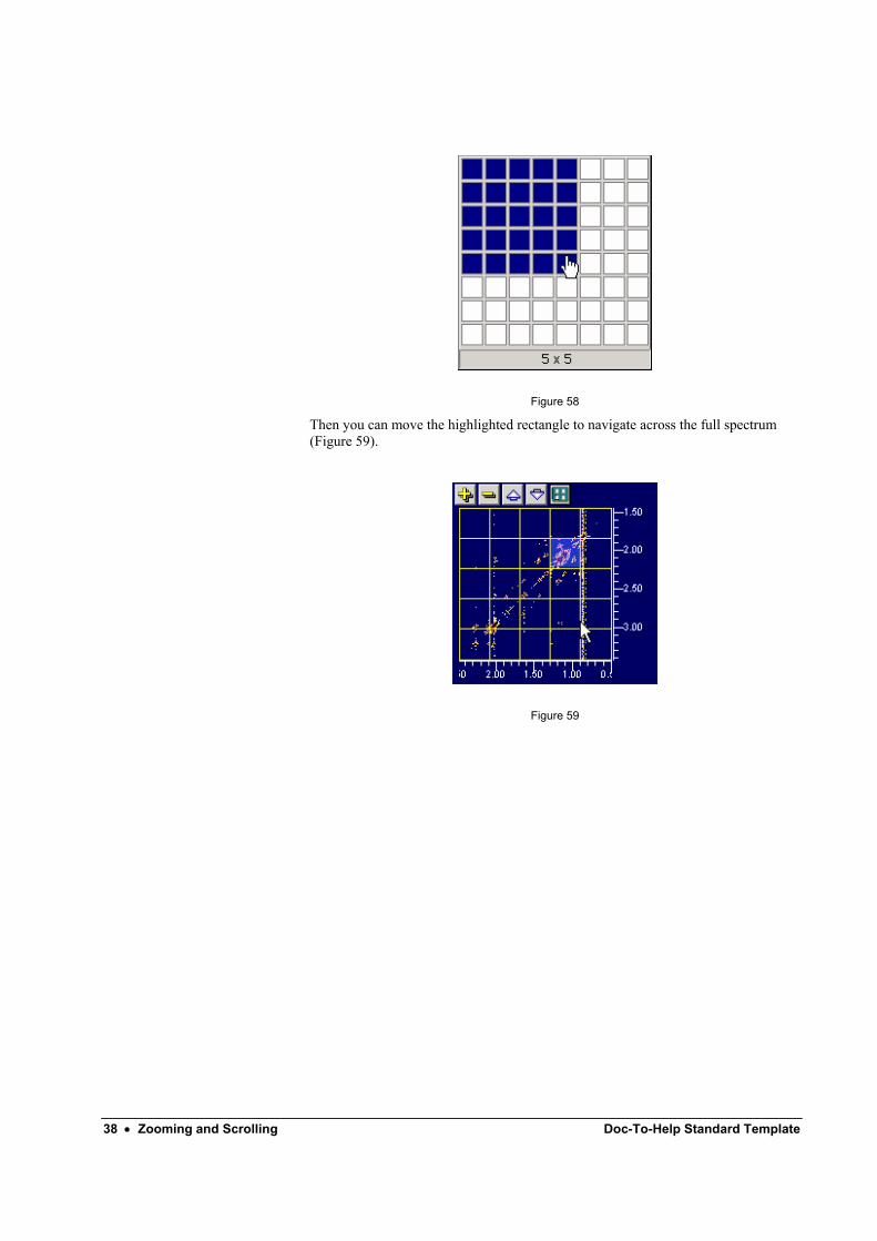
Splits the Full View Window in a grid using a pop-up control that allows you to set the number of rows and columns, up to 8x8 (Figure 58).
38 • Zooming and Scrolling Doc-To-Help Standard Template
Figure 58
Then you can move the highlighted rectangle to navigate across the full spectrum (Figure 59).
Figure 59
MestRe-C Fourier Transform (FT) and related functions • 39
Fourier Transform (FT) and related functions
Introduction
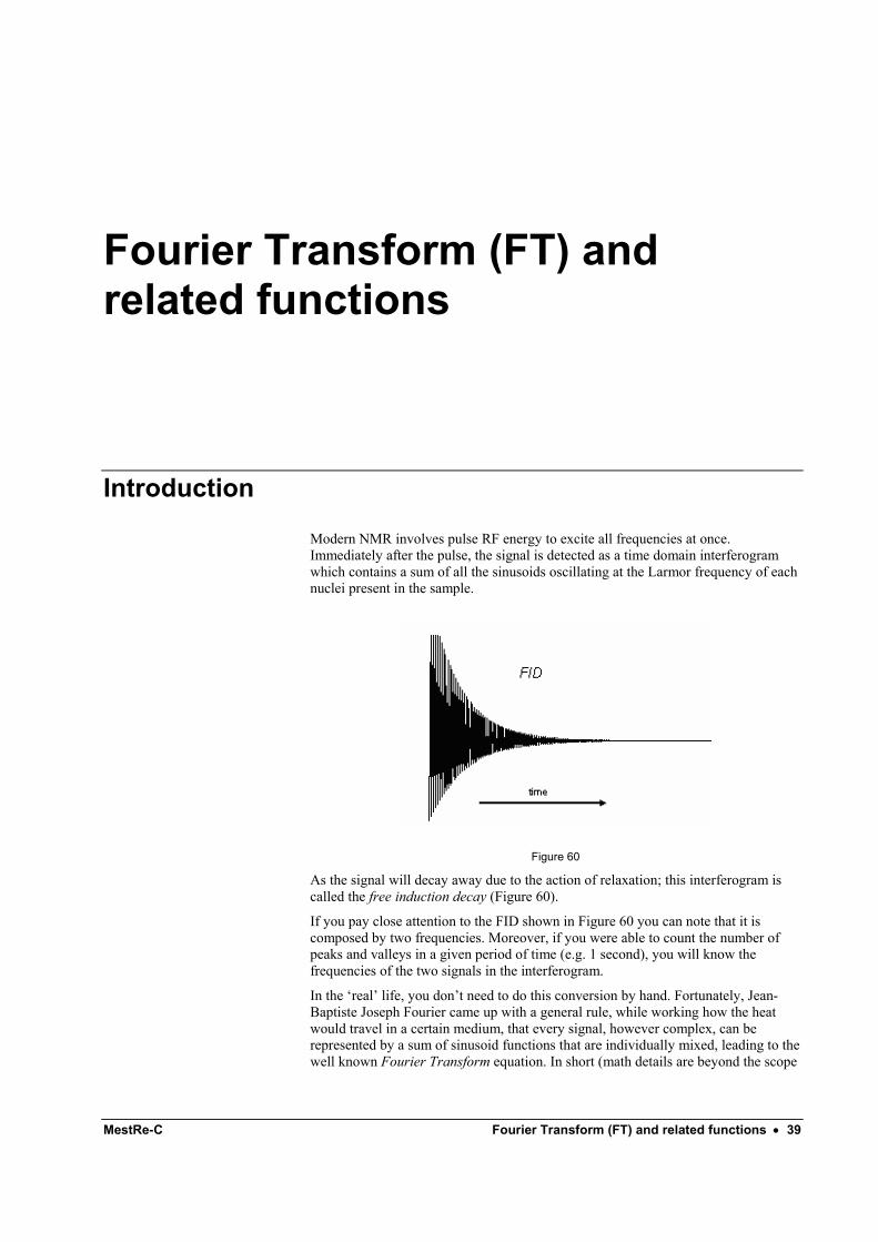
Modern NMR involves pulse RF energy to excite all frequencies at once. Immediately after the pulse, the signal is detected as a time domain interferogram which contains a sum of all the sinusoids oscillating at the Larmor frequency of each nuclei present in the sample.
Figure 60
As the signal will decay away due to the action of relaxation; this interferogram is called the free induction decay (Figure 60).
If you pay close attention to the FID shown in Figure 60 you can note that it is composed by two frequencies. Moreover, if you were able to count the number of peaks and valleys in a given period of time (e.g. 1 second), you will know the frequencies of the two signals in the interferogram.
In the ‘real’ life, you don’t need to do this conversion by hand. Fortunately, Jean-Baptiste Joseph Fourier came up with a general rule, while working how the heat would travel in a certain medium, that every signal, however complex, can be represented by a sum of sinusoid functions that are individually mixed, leading to the well known Fourier Transform equation. In short (math details are beyond the scope
40 • Fourier Transform (FT) and related functions Doc-To-Help Standard Template
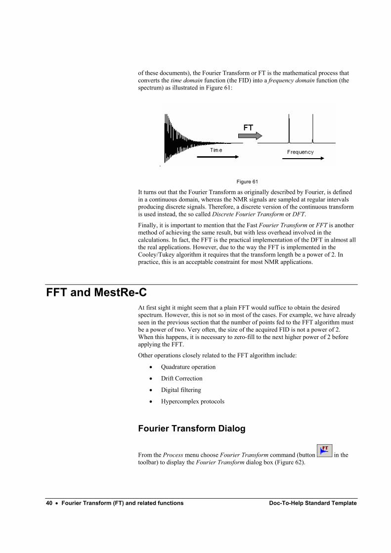
of these documents), the Fourier Transform or FT is the mathematical process that converts the time domain function (the FID) into a frequency domain function (the spectrum) as illustrated in Figure 61:
.
Figure 61
It turns out that the Fourier Transform as originally described by Fourier, is defined in a continuous domain, whereas the NMR signals are sampled at regular intervals producing discrete signals. Therefore, a discrete version of the continuous transform is used instead, the so called Discrete Fourier Transform or DFT.
Finally, it is important to mention that the Fast Fourier Transform or FFT is another method of achieving the same result, but with less overhead involved in the calculations. In fact, the FFT is the practical implementation of the DFT in almost all the real applications. However, due to the way the FFT is implemented in the Cooley/Tukey algorithm it requires that the transform length be a power of 2. In practice, this is an acceptable constraint for most NMR applications.
FFT and MestRe-C At first sight it might seem that a plain FFT would suffice to obtain the desired spectrum. However, this is not so in most of the cases. For example, we have already seen in the previous section that the number of points fed to the FFT algorithm must be a power of two. Very often, the size of the acquired FID is not a power of 2. When this happens, it is necessary to zero-fill to the next higher power of 2 before applying the FFT.
Other operations closely related to the FFT algorithm include:
• Quadrature operation
• Drift Correction
• Digital filtering
• Hypercomplex protocols
Fourier Transform Dialog
From the Process menu choose Fourier Transform command (button in the toolbar) to display the Fourier Transform dialog box (Figure 62).
MestRe-C Fourier Transform (FT) and related functions • 41
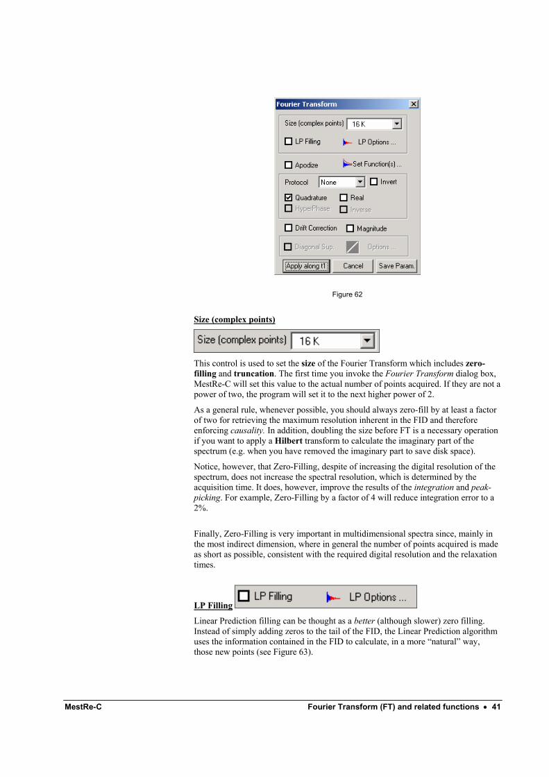
Figure 62
Size (complex points)
This control is used to set the size of the Fourier Transform which includes zero-filling and truncation. The first time you invoke the Fourier Transform dialog box, MestRe-C will set this value to the actual number of points acquired. If they are not a power of two, the program will set it to the next higher power of 2.
As a general rule, whenever possible, you should always zero-fill by at least a factor of two for retrieving the maximum resolution inherent in the FID and therefore enforcing causality. In addition, doubling the size before FT is a necessary operation if you want to apply a Hilbert transform to calculate the imaginary part of the spectrum (e.g. when you have removed the imaginary part to save disk space).
Notice, however, that Zero-Filling, despite of increasing the digital resolution of the spectrum, does not increase the spectral resolution, which is determined by the acquisition time. It does, however, improve the results of the integration and peak-picking. For example, Zero-Filling by a factor of 4 will reduce integration error to a 2%.
Finally, Zero-Filling is very important in multidimensional spectra since, mainly in the most indirect dimension, where in general the number of points acquired is made as short as possible, consistent with the required digital resolution and the relaxation times.
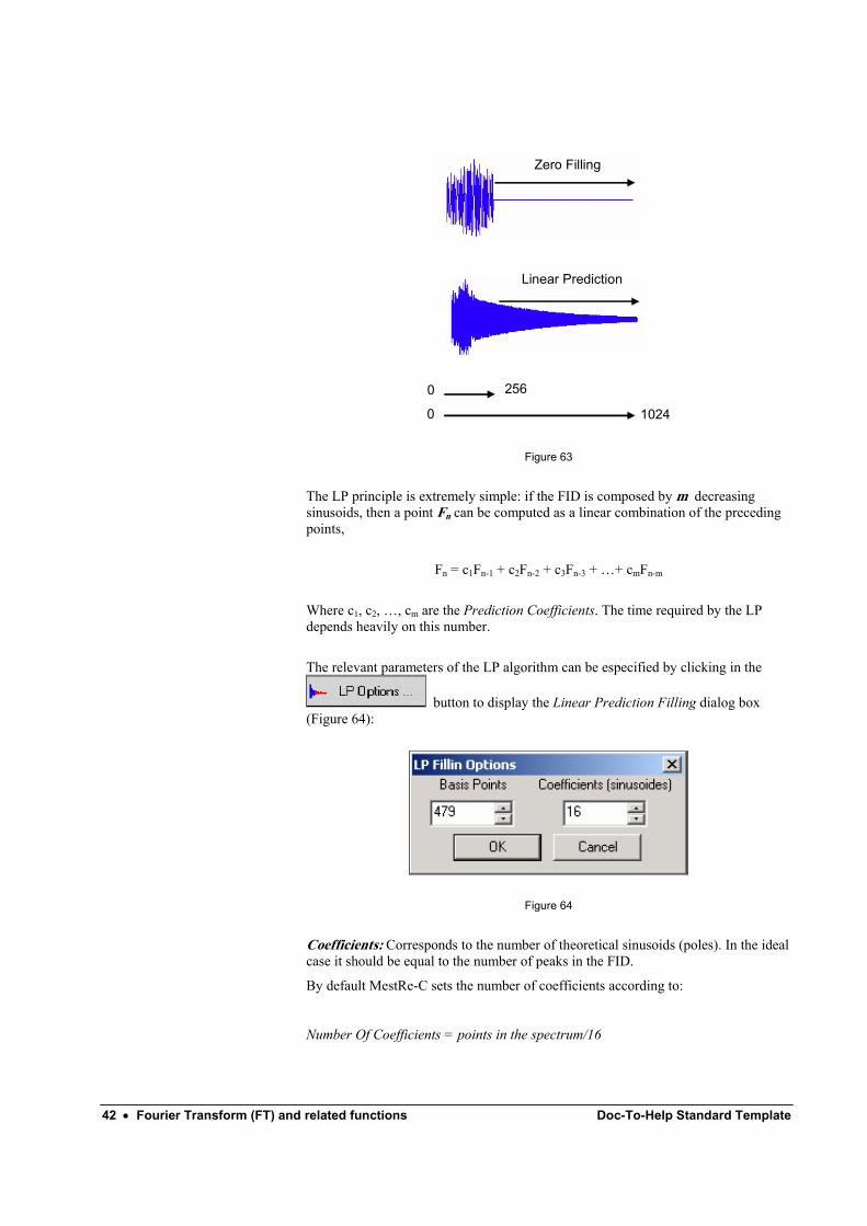
LP Filling
Linear Prediction filling can be thought as a better (although slower) zero filling. Instead of simply adding zeros to the tail of the FID, the Linear Prediction algorithm uses the information contained in the FID to calculate, in a more “natural” way, those new points (see Figure 63).
42 • Fourier Transform (FT) and related functions Doc-To-Help Standard Template
0
0
256
1024
Zero Filling
Linear Prediction
Figure 63
The LP principle is extremely simple: if the FID is composed by m decreasing sinusoids, then a point Fn can be computed as a linear combination of the preceding points,
Fn = c1Fn-1 + c2Fn-2 + c3Fn-3 + …+ cmFn-m
Where c1, c2, …, cm are the Prediction Coefficients. The time required by the LP depends heavily on this number.
The relevant parameters of the LP algorithm can be especified by clicking in the
button to display the Linear Prediction Filling dialog box (Figure 64):
Figure 64
Coefficients: Corresponds to the number of theoretical sinusoids (poles). In the ideal case it should be equal to the number of peaks in the FID.
By default MestRe-C sets the number of coefficients according to:
Number Of Coefficients = points in the spectrum/16

MestRe-C Fourier Transform (FT) and related functions • 43
And if this number is higher than 16, then it will be truncated to this value. You can enter any other value but take into account that the time required by the LP depends heavily on this number so use less coefficients if you want to save time.
Basis Points: Corresponds to the number of ‘good’ experimental points to be entered in the calculations. Their number should be at least two or three times greater than the number of coefficients. In this case of Linear Prediction Filling, MestRe-C computes this number according to the following formula:
Number Of Basis Points = points in the spectrum - coefficients – 1
44 • Fourier Transform (FT) and related functions Doc-To-Help Standard Template
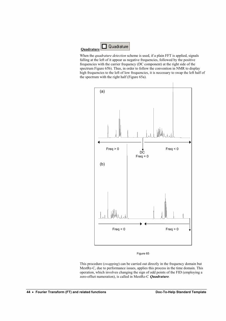
Quadrature
When the quadrature detection scheme is used, if a plain FFT is applied, signals falling at the left of it appear as negative frequencies, followed by the positive frequencies with the carrier frequency (DC component) at the right side of the spectrum Figure 65b). Thus, in order to follow the convention in NMR to display high frequencies to the left of low frequencies, it is necessary to swap the left half of the spectrum with the right half (Figure 65a).
Freq > 0 Freq < 0 DC
Freq = 0
Freq < 0 Freq > 0
(a)
(b)
Figure 65
This procedure (swapping) can be carried out directly in the frequency domain but MestRe-C, due to performance issues, applies this process in the time domain. This operation, which involves changing the sign of odd points of the FID (employing a zero-offset numeration), is called in MestRe-C Quadrature.
MestRe-C Fourier Transform (FT) and related functions • 45
The Quadrature option should always be checked in most NMR experiments. A exception to this rule is for the f1 dimension of spectra acquired in TPPI mode. In addition, it is possible that this operation had been already performed in the spectrometer; in this case don’t do it a second time!.
Protocol
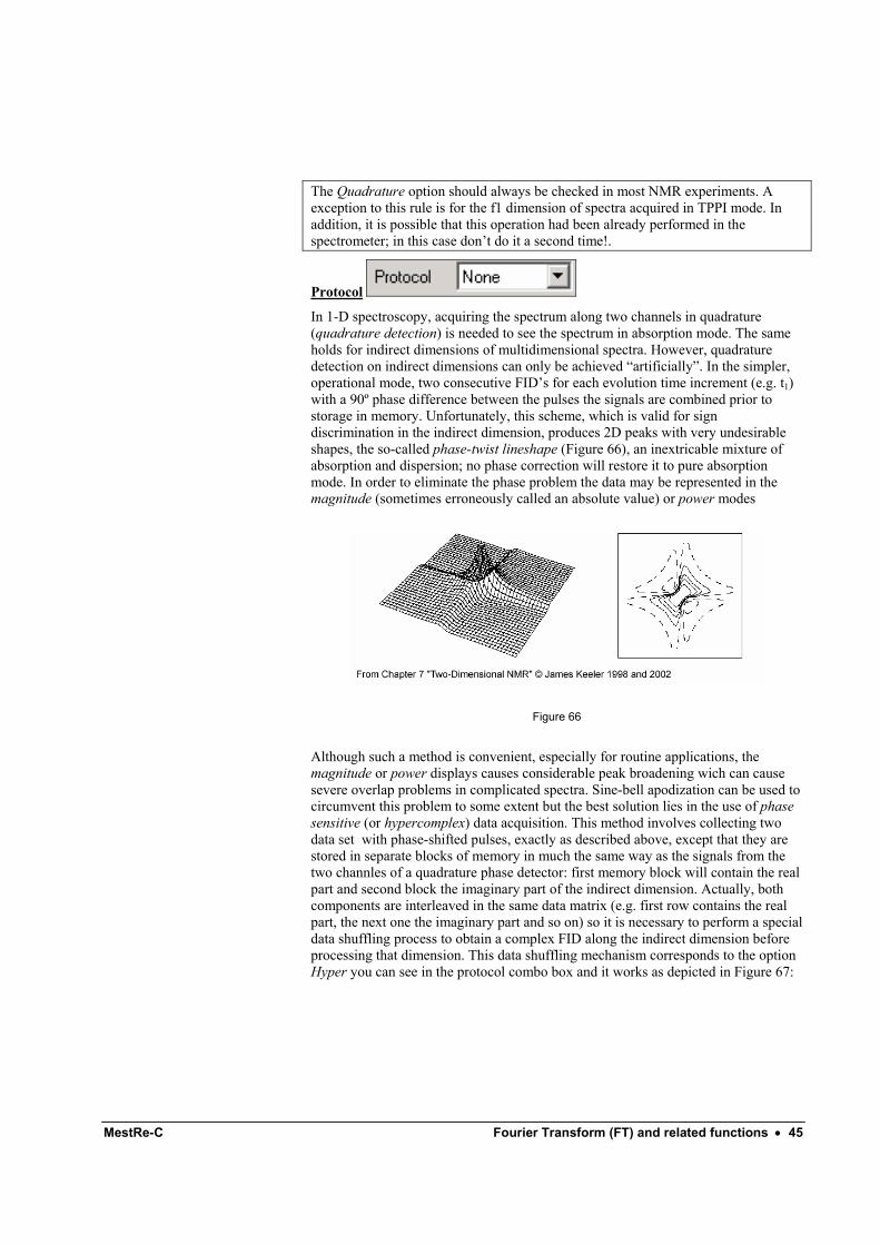
In 1-D spectroscopy, acquiring the spectrum along two channels in quadrature (quadrature detection) is needed to see the spectrum in absorption mode. The same holds for indirect dimensions of multidimensional spectra. However, quadrature detection on indirect dimensions can only be achieved “artificially”. In the simpler, operational mode, two consecutive FID’s for each evolution time increment (e.g. t1) with a 90º phase difference between the pulses the signals are combined prior to storage in memory. Unfortunately, this scheme, which is valid for sign discrimination in the indirect dimension, produces 2D peaks with very undesirable shapes, the so-called phase-twist lineshape (Figure 66), an inextricable mixture of absorption and dispersion; no phase correction will restore it to pure absorption mode. In order to eliminate the phase problem the data may be represented in the magnitude (sometimes erroneously called an absolute value) or power modes
Figure 66
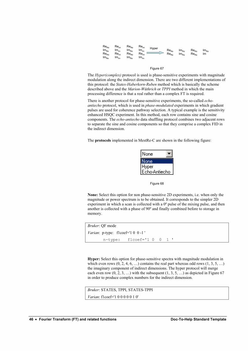
Although such a method is convenient, especially for routine applications, the magnitude or power displays causes considerable peak broadening wich can cause severe overlap problems in complicated spectra. Sine-bell apodization can be used to circumvent this problem to some extent but the best solution lies in the use of phase sensitive (or hypercomplex) data acquisition. This method involves collecting two data set with phase-shifted pulses, exactly as described above, except that they are stored in separate blocks of memory in much the same way as the signals from the two channles of a quadrature phase detector: first memory block will contain the real part and second block the imaginary part of the indirect dimension. Actually, both components are interleaved in the same data matrix (e.g. first row contains the real part, the next one the imaginary part and so on) so it is necessary to perform a special data shuffling process to obtain a complex FID along the indirect dimension before processing that dimension. This data shuffling mechanism corresponds to the option Hyper you can see in the protocol combo box and it works as depicted in Figure 67:
46 • Fourier Transform (FT) and related functions Doc-To-Help Standard Template
ReRe ReIm ReRe ReImImRe ImIm ImRe ImImReRe ReIm ReRe ReImImRe ImIm ImRe ImIm
ReRe ImRe ReRe ImReReRe ImRe ReRe Im
Hyper
Figure 67
The Hyper(complex) protocol is used is phase-sensitive experiments with magnitude modulation along the indirect dimension. There are two different implementations of this protocol: the States-Haberkorn-Ruben method which is basically the scheme described above and the Marion-Wüthrich or TPPI method in which the main processing difference is that a real rather than a complex FT is required.
There is another protocol for phase-sensitive experiments, the so-called echo-antiecho protocol, which is used in phase-modulated experiments in which gradient pulses are used for coherence pathway selection. A typical example is the sensitivity enhanced HSQC experiment. In this method, each row contains sine and cosine components. The echo-antiecho data shuffling protocol combines two adjacent rows to separate the sine and cosine components so that they comprise a complex FID in the indirect dimension.
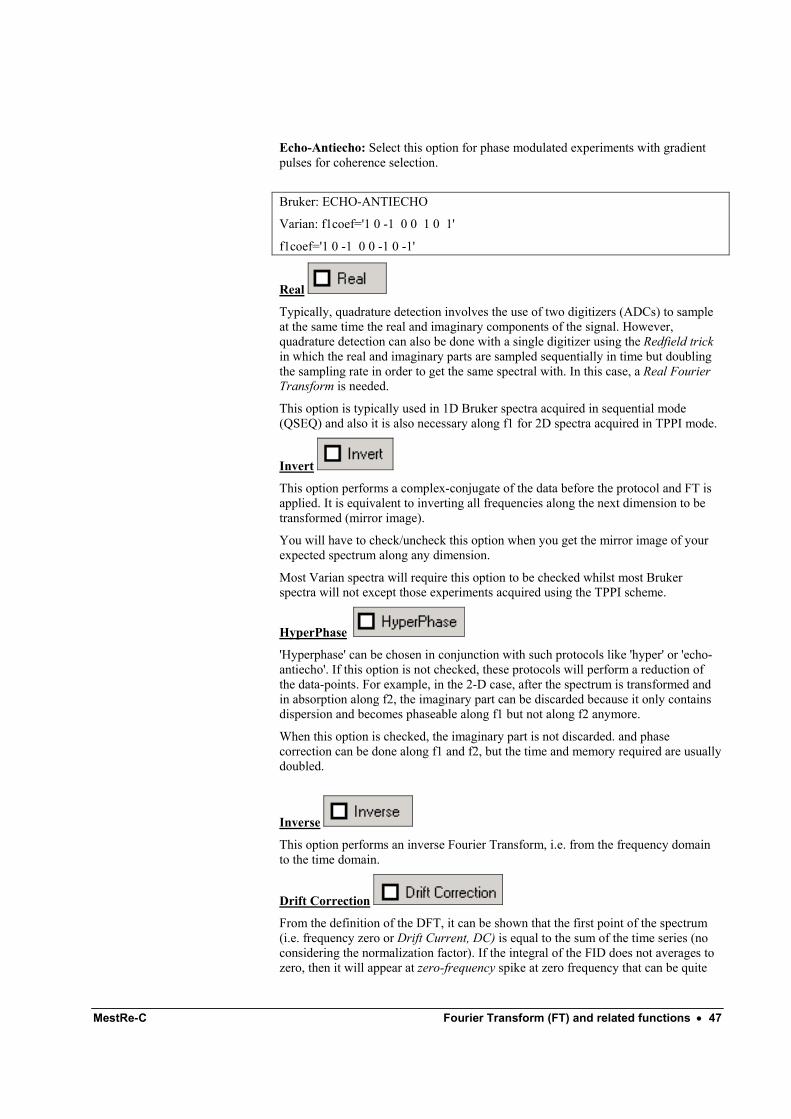
The protocols implemented in MestRe-C are shown in the following figure:
Figure 68
None: Select this option for non phase-sensitive 2D experiments, i.e. when only the magnitude or power spectrum is to be obtained. It corresponds to the simpler 2D experiment in which a scan is collected with a 0º pulse of the mixing pulse, and then another is collected with a phase of 90º and finally combined before to storage in memory.
Bruker: QF mode
Varian: p-type: f1coef='1 0 0 -1 '
n-type: f1coef='1 0 0 1 '
Hyper: Select this option for phase-sensitive spectra with magnitude modulation in which even rows (0, 2, 4, 6, …) contains the real part whereas odd rows (1, 3, 5, …) the imaginary component of indirect dimensions. The hyper protocol will merge each even row (0, 2, 3, …) with the subsequent (1, 3, 5, …) as depicted in Figure 67 in order to produce complex numbers for the indirect dimension.
Bruker: STATES, TPPI, STATES-TPPI
Varian: f1coef='1 0 0 0 0 0 1 0'
MestRe-C Fourier Transform (FT) and related functions • 47
Echo-Antiecho: Select this option for phase modulated experiments with gradient pulses for coherence selection.
Bruker: ECHO-ANTIECHO
Varian: f1coef='1 0 -1 0 0 1 0 1'
f1coef='1 0 -1 0 0 -1 0 -1'
Real
Typically, quadrature detection involves the use of two digitizers (ADCs) to sample at the same time the real and imaginary components of the signal. However, quadrature detection can also be done with a single digitizer using the Redfield trick in which the real and imaginary parts are sampled sequentially in time but doubling the sampling rate in order to get the same spectral with. In this case, a Real Fourier Transform is needed.
This option is typically used in 1D Bruker spectra acquired in sequential mode (QSEQ) and also it is also necessary along f1 for 2D spectra acquired in TPPI mode.
Invert
This option performs a complex-conjugate of the data before the protocol and FT is applied. It is equivalent to inverting all frequencies along the next dimension to be transformed (mirror image).
You will have to check/uncheck this option when you get the mirror image of your expected spectrum along any dimension.
Most Varian spectra will require this option to be checked whilst most Bruker spectra will not except those experiments acquired using the TPPI scheme.
HyperPhase
'Hyperphase' can be chosen in conjunction with such protocols like 'hyper' or 'echo-antiecho'. If this option is not checked, these protocols will perform a reduction of the data-points. For example, in the 2-D case, after the spectrum is transformed and in absorption along f2, the imaginary part can be discarded because it only contains dispersion and becomes phaseable along f1 but not along f2 anymore.
When this option is checked, the imaginary part is not discarded. and phase correction can be done along f1 and f2, but the time and memory required are usually doubled.
Inverse
This option performs an inverse Fourier Transform, i.e. from the frequency domain to the time domain.
Drift Correction
From the definition of the DFT, it can be shown that the first point of the spectrum (i.e. frequency zero or Drift Current, DC) is equal to the sum of the time series (no considering the normalization factor). If the integral of the FID does not averages to zero, then it will appear at zero-frequency spike at zero frequency that can be quite
48 • Fourier Transform (FT) and related functions Doc-To-Help Standard Template
annoying. In order to remove such a spurious peak it is necessary to bring the FID level offset to zero. This is done by averaging the last part (e.g. last 5%) of the FID to determine a mean DC level –the real and imaginary averages are computed separately- which is then subtracted from the full FID.
DC correction is disabled in 2D experiments because this method is accurate only when the FID is long enough and the signal decays, which is not the case in most of the 2D NMR spectra.
Magnitude
The 'Magnitude' determines the representation of the final spectrum. If checked you will see the absolute part of the spectrum; if unchecked you will see the real part. You are free to perform or to undo the choice afterwards. (It is unrelated to the FT).
Diagonal Suppression
MestRe-C Window Functions - Apodization • 49
Window Functions - Apodization
Introduction Window functions are used to enhance the resolution or the sensitivity (S/N ratio) in the spectrum or to remove truncation artefacts. They can also be useful to change the lineshape into a more desirable form.
Typically, in 1D spectroscopy you will be interested in improving resolution and/or sensitivity.
In the case of nD spectroscopy in which the FID may be highly truncated, specially along the indirect dimensions, you will be interested in apodizing to avoid the wiggles typical of the truncation problem (literally “chopping off the feet” in Greek).
In MestRe-C is possible to choose among several window functions which can also be applied simultaneously.
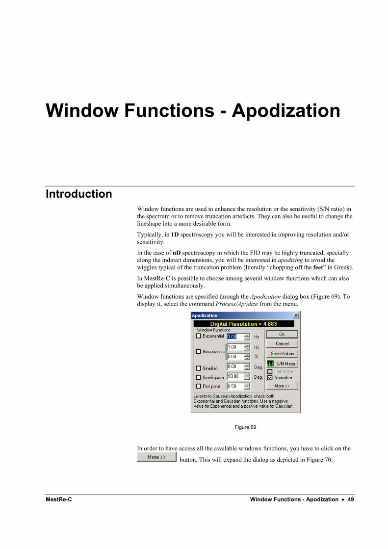
Window functions are specified through the Apodization dialog box (Figure 69). To display it, select the command Process/Apodize from the menu.
Figure 69
In order to have access all the available windows functions, you have to click on the
button. This will expand the dialog as depicted in Figure 70:
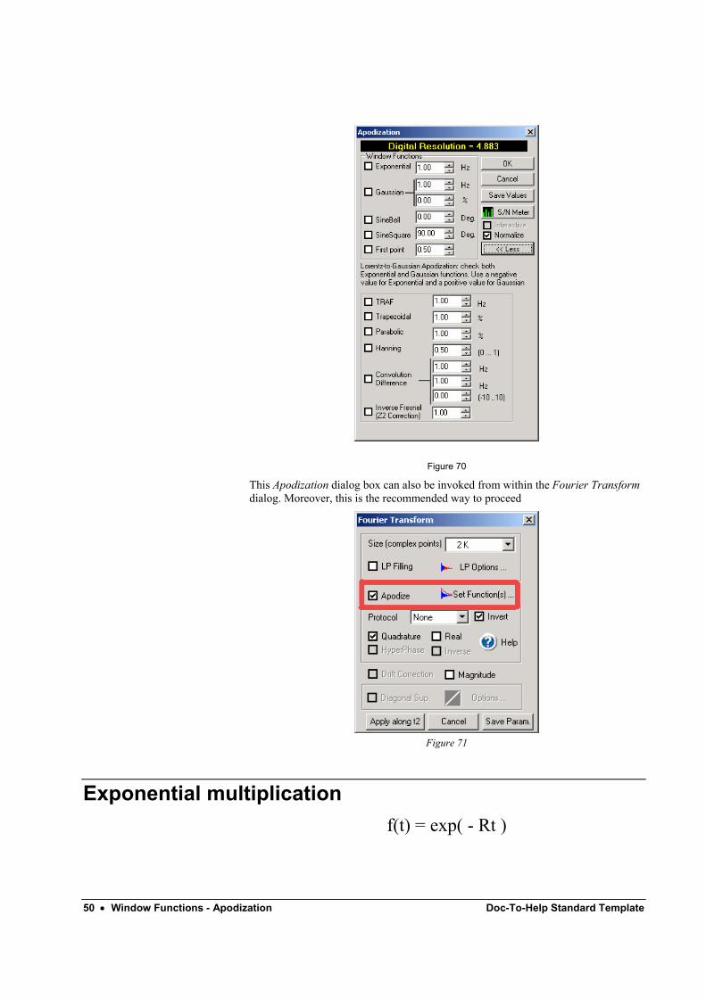
50 • Window Functions - Apodization Doc-To-Help Standard Template
Figure 70
This Apodization dialog box can also be invoked from within the Fourier Transform dialog. Moreover, this is the recommended way to proceed
Figure 71
Exponential multiplication f(t) = exp( - Rt )
MestRe-C Window Functions - Apodization • 51
This function needs only one parameter that corresponds to the line broadening in Hz (R in the equation).
The line in the corresponding transformed spectrum is of width (R/π) Hz.
A positive value will increase the sensitivity (i.e. S/N) but it will increase the linewidth (i.e. it will reduce the resolution). For example, a value of 1.0 Hz will increase the linewidth of the spectrum by 1 Hz.
A negative value has the opposite effect: it will reduce the linewidth (i.e. it will increase the resolution) but at the expense of decreasing the sensitivity. However, this may lead to a seriously enhanced noise component and to truncation artifacts when zero filling is used. For this reason, it is normally used in combination with some other function (like the gaussian).
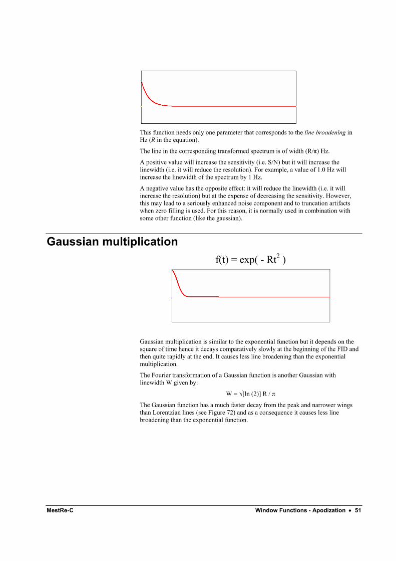
Gaussian multiplication f(t) = exp( - Rt2 )
Gaussian multiplication is similar to the exponential function but it depends on the square of time hence it decays comparatively slowly at the beginning of the FID and then quite rapidly at the end. It causes less line broadening than the exponential multiplication.
The Fourier transformation of a Gaussian function is another Gaussian with linewidth W given by:
W = √[ln (2)] R / π
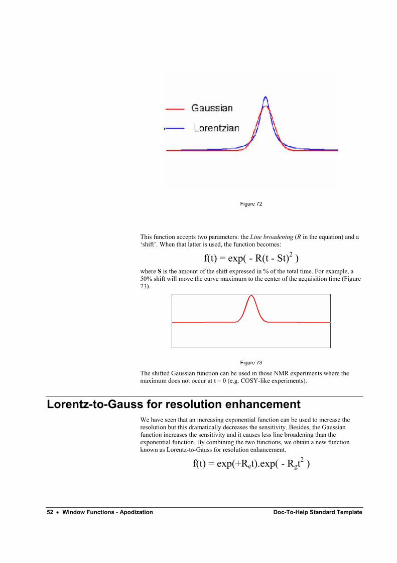
The Gaussian function has a much faster decay from the peak and narrower wings than Lorentzian lines (see Figure 72) and as a consequence it causes less line broadening than the exponential function.
52 • Window Functions - Apodization Doc-To-Help Standard Template
Figure 72
This function accepts two parameters: the Line broadening (R in the equation) and a ‘shift’. When that latter is used, the function becomes:
f(t) = exp( - R(t - St)2 ) where S is the amount of the shift expressed in % of the total time. For example, a 50% shift will move the curve maximum to the center of the acquisition time (Figure 73).
Figure 73
The shifted Gaussian function can be used in those NMR experiments where the maximum does not occur at t = 0 (e.g. COSY-like experiments).
Lorentz-to-Gauss for resolution enhancement We have seen that an increasing exponential function can be used to increase the resolution but this dramatically decreases the sensitivity. Besides, the Gaussian function increases the sensitivity and it causes less line broadening than the exponential function. By combining the two functions, we obtain a new function known as Lorentz-to-Gauss for resolution enhancement.
f(t) = exp(+Ret).exp( - Rgt2 )
MestRe-C Window Functions - Apodization • 53
This function is not directly implemented in MestRe-C but you can apply it by checking both the Exponential and Gaussian multiplication functions and introducing a negative value for the Exponential line broadening (Re) and a positive value for the Gaussian parameter (Rg).
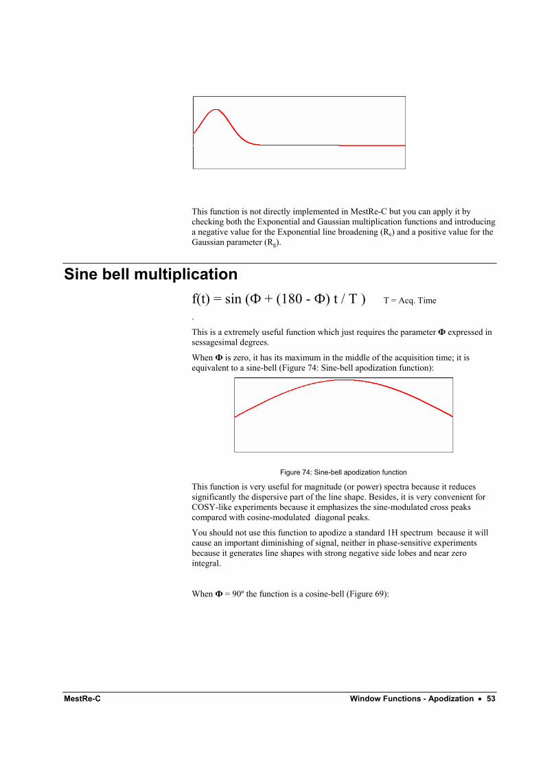
Sine bell multiplication f(t) = sin (Ф + (180 - Ф) t / T ) T = Acq. Time
.
This is a extremely useful function which just requires the parameter Ф expressed in sessagesimal degrees.
When Ф is zero, it has its maximum in the middle of the acquisition time; it is equivalent to a sine-bell (Figure 74: Sine-bell apodization function):
Figure 74: Sine-bell apodization function
This function is very useful for magnitude (or power) spectra because it reduces significantly the dispersive part of the line shape. Besides, it is very convenient for COSY-like experiments because it emphasizes the sine-modulated cross peaks compared with cosine-modulated diagonal peaks.
You should not use this function to apodize a standard 1H spectrum because it will cause an important diminishing of signal, neither in phase-sensitive experiments because it generates line shapes with strong negative side lobes and near zero integral.
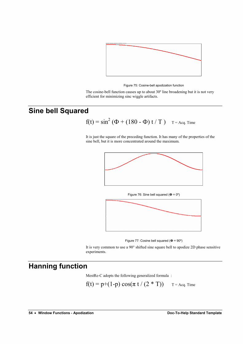
When Ф = 90º the function is a cosine-bell (Figure 69):
54 • Window Functions - Apodization Doc-To-Help Standard Template
Figure 75: Cosine-bell apodization function
The cosine-bell function causes up to about 30º line broadening but it is not very efficient for minimizing sinc wiggle artifacts.
Sine bell Squared f(t) = sin2 (Ф + (180 - Ф) t / T ) T = Acq. Time
It is just the square of the preceding function. It has many of the properties of the sine bell, but it is more concentrated around the maximum.
Figure 76: Sine bell squared (Ф = 0º)
Figure 77: Cosine bell squared (Ф = 90º)
It is very common to use a 90° shifted sine square bell to apodize 2D phase sensitive experiments.
Hanning function MestRe-C adopts the following generalized formula :
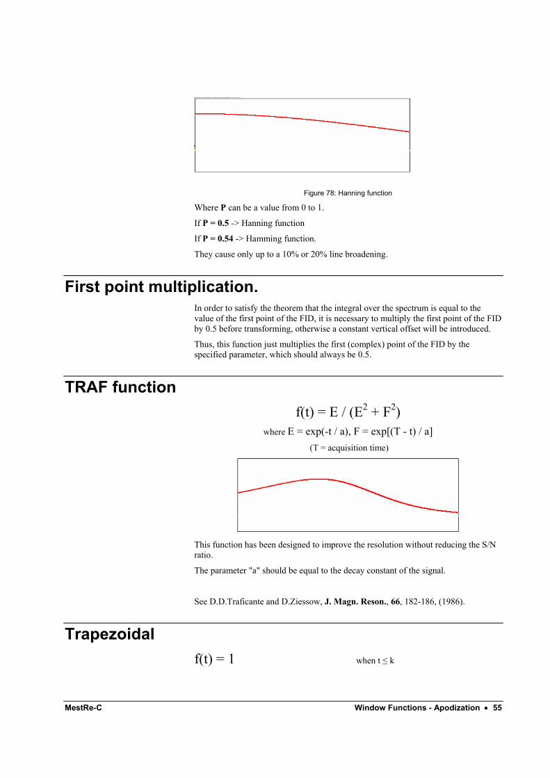
f(t) = p+(1-p) cos(π t / (2 * T)) T = Acq. Time
MestRe-C Window Functions - Apodization • 55
Figure 78: Hanning function
Where P can be a value from 0 to 1.
If P = 0.5 -> Hanning function
If P = 0.54 -> Hamming function.
They cause only up to a 10% or 20% line broadening.
First point multiplication. In order to satisfy the theorem that the integral over the spectrum is equal to the value of the first point of the FID, it is necessary to multiply the first point of the FID by 0.5 before transforming, otherwise a constant vertical offset will be introduced.
Thus, this function just multiplies the first (complex) point of the FID by the specified parameter, which should always be 0.5.
TRAF function f(t) = E / (E2 + F2)
where E = exp(-t / a), F = exp[(T - t) / a]
(T = acquisition time)
This function has been designed to improve the resolution without reducing the S/N ratio.
The parameter "a" should be equal to the decay constant of the signal.
See D.D.Traficante and D.Ziessow, J. Magn. Reson., 66, 182-186, (1986).
Trapezoidal f(t) = 1 when t ≤ k
56 • Window Functions - Apodization Doc-To-Help Standard Template
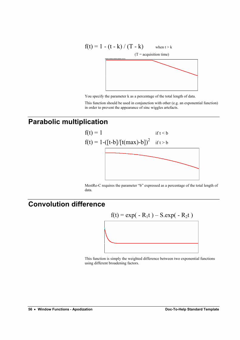
f(t) = 1 - (t - k) / (T - k) when t > k
(T = acquisition time)
You specify the parameter k as a percentage of the total length of data.
This function should be used in conjunction with other (e.g. an exponential function) in order to prevent the appearance of sinc wiggles artefacts.
Parabolic multiplication f(t) = 1 if t < b
f(t) = 1-([t-b]/[t(max)-b])2 if t > b
MestRe-C requires the parameter “b” expressed as a percentage of the total length of data.
Convolution difference f(t) = exp( - R1t ) – S.exp( - R2t )
This function is simply the weighted difference between two exponential functions using different broadening factors.
MestRe-C Window Functions - Apodization • 57
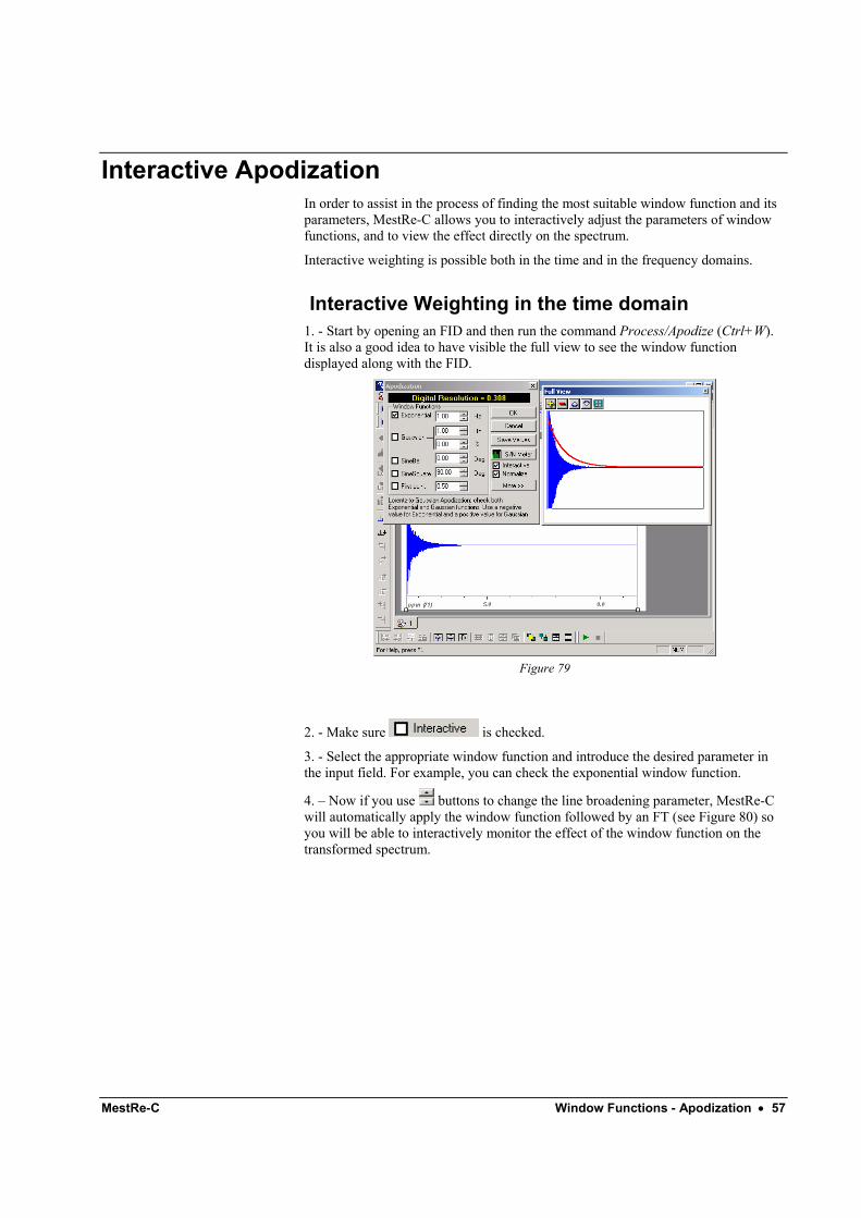
Interactive Apodization In order to assist in the process of finding the most suitable window function and its parameters, MestRe-C allows you to interactively adjust the parameters of window functions, and to view the effect directly on the spectrum.
Interactive weighting is possible both in the time and in the frequency domains.
Interactive Weighting in the time domain 1. - Start by opening an FID and then run the command Process/Apodize (Ctrl+W). It is also a good idea to have visible the full view to see the window function displayed along with the FID.
Figure 79
2. - Make sure is checked.
3. - Select the appropriate window function and introduce the desired parameter in the input field. For example, you can check the exponential window function.
4. – Now if you use buttons to change the line broadening parameter, MestRe-C will automatically apply the window function followed by an FT (see Figure 80) so you will be able to interactively monitor the effect of the window function on the transformed spectrum.
58 • Window Functions - Apodization Doc-To-Help Standard Template
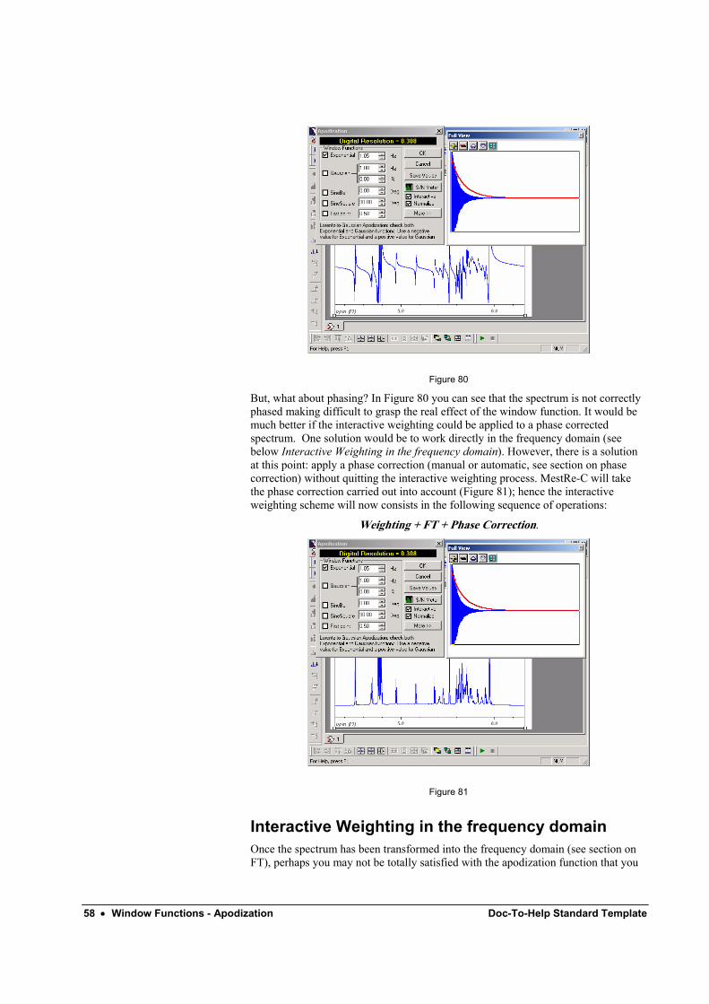
Figure 80
But, what about phasing? In Figure 80 you can see that the spectrum is not correctly phased making difficult to grasp the real effect of the window function. It would be much better if the interactive weighting could be applied to a phase corrected spectrum. One solution would be to work directly in the frequency domain (see below Interactive Weighting in the frequency domain). However, there is a solution at this point: apply a phase correction (manual or automatic, see section on phase correction) without quitting the interactive weighting process. MestRe-C will take the phase correction carried out into account (Figure 81); hence the interactive weighting scheme will now consists in the following sequence of operations:
Weighting + FT + Phase Correction.
Figure 81
Interactive Weighting in the frequency domain Once the spectrum has been transformed into the frequency domain (see section on FT), perhaps you may not be totally satisfied with the apodization function that you

MestRe-C Window Functions - Apodization • 59
have chosen and you would like to change it. Typically, you will run the command Process/Apodize. MestRe-C automatically will reload the original FID in order to start over all the processing. MestRe-C will remember all the processing operations that you had performed previously, so you just need to select the new values for the apodization function. Note that you will have to activate the check box if you want to get the transformed spectrum directly.
In addition to this approach, there yet is another command that can be used to re-apodize your spectrum without the need to reload the original data set. This command is Process/Weight by eye. Rather than reloading the FID, this command performs an inverse FT on the spectrum and then follows as before. The main problem of this method is that the inverse FT does not lead exactly to the original data points. Before applying the inverse FT it is necessary to reverse the window function that was previously applied to the data. In some cases, especially if the apodization function that has been applied decays too fast (i.e. a high value for the line broadening parameter has been used), then the process of reverting the apodization function may lead to some instabilities which can create artefacts at the end of the FID.
..

MestRe-C Phase Correction • 61
Phase Correction
Introduction Phase correction is the process which mixes the real and imaginary components of the spectrum in order to obtain pure phase lineshapes. The correction is composed of a frequency independent, or zero phase correction ( 0Φ ) and a first order, or linear
dependent on the frequency, phase correction ( 1Φ ).
This mixing process consist in multiplying each spectral point n by the complex number
)/)(( 10 Njnie Φ−+Φ
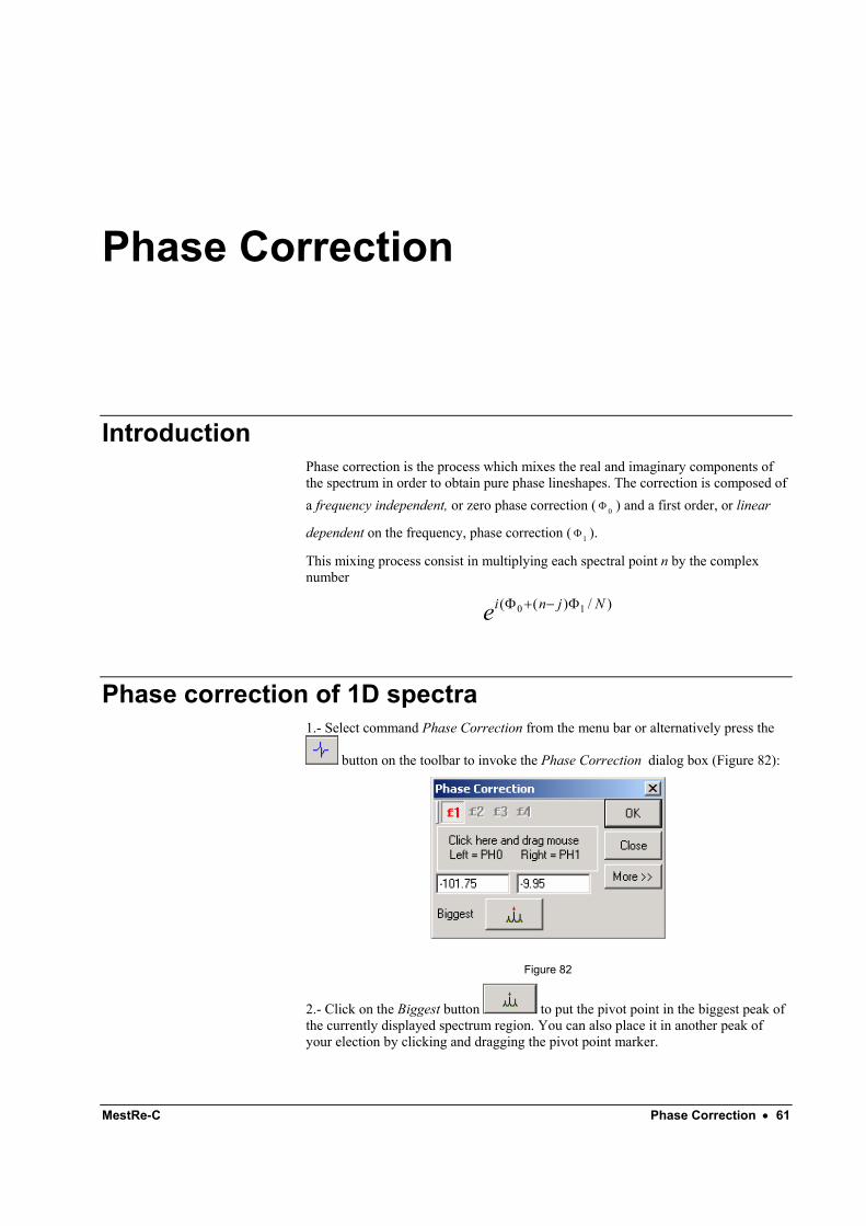
Phase correction of 1D spectra 1.- Select command Phase Correction from the menu bar or alternatively press the
button on the toolbar to invoke the Phase Correction dialog box (Figure 82):
Figure 82
2.- Click on the Biggest button to put the pivot point in the biggest peak of the currently displayed spectrum region. You can also place it in another peak of your election by clicking and dragging the pivot point marker.
62 • Phase Correction Doc-To-Help Standard Template
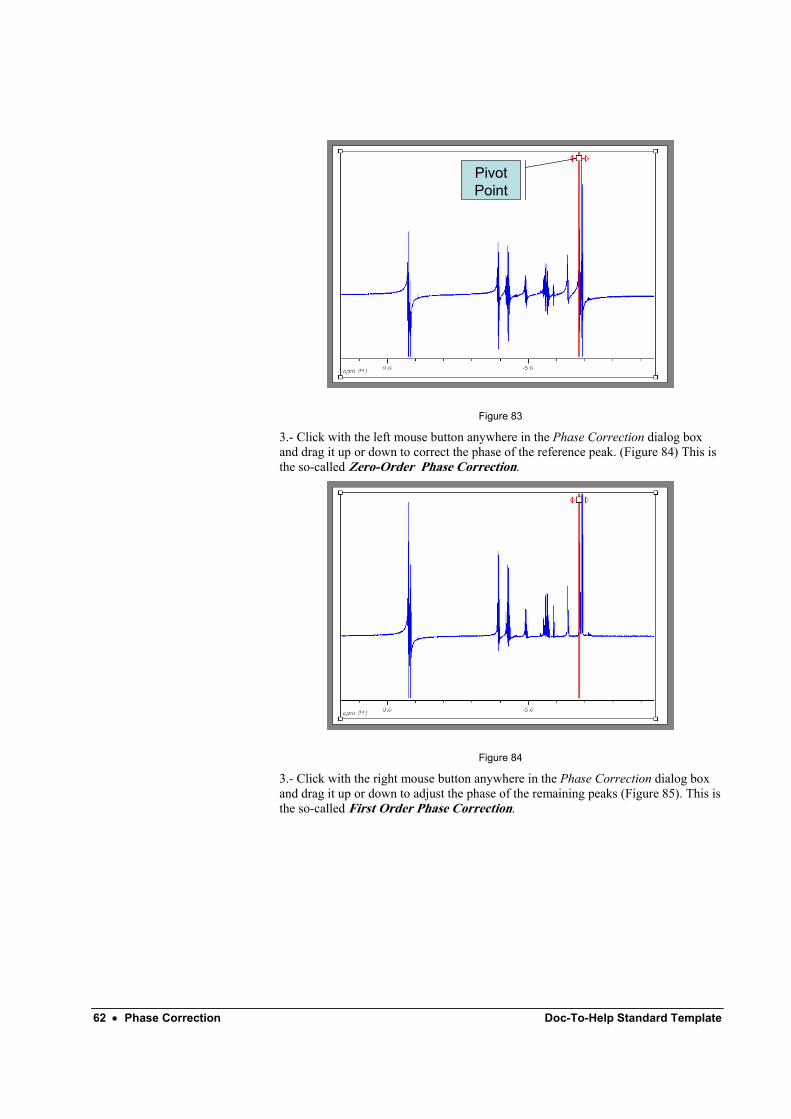
Pivot Point
Figure 83
3.- Click with the left mouse button anywhere in the Phase Correction dialog box and drag it up or down to correct the phase of the reference peak. (Figure 84) This is the so-called Zero-Order Phase Correction.
Figure 84
3.- Click with the right mouse button anywhere in the Phase Correction dialog box and drag it up or down to adjust the phase of the remaining peaks (Figure 85). This is the so-called First Order Phase Correction.
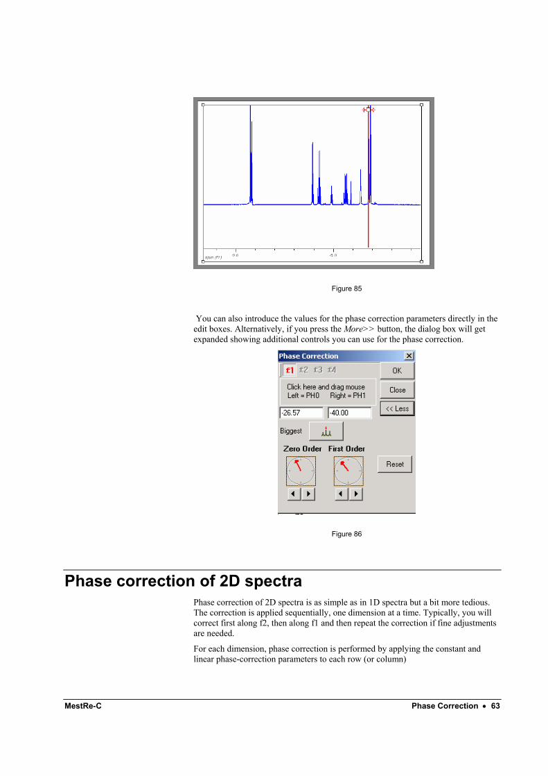
MestRe-C Phase Correction • 63
Figure 85
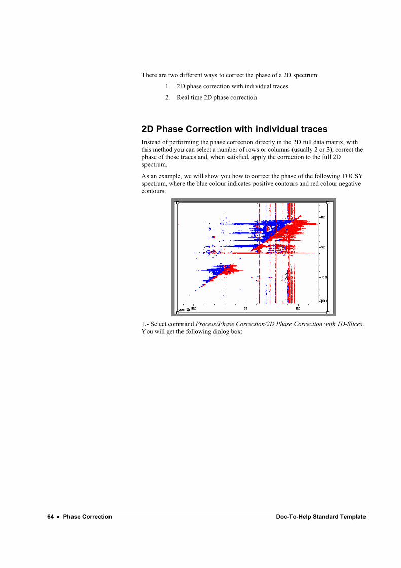
You can also introduce the values for the phase correction parameters directly in the edit boxes. Alternatively, if you press the More>> button, the dialog box will get expanded showing additional controls you can use for the phase correction.
Figure 86
Phase correction of 2D spectra Phase correction of 2D spectra is as simple as in 1D spectra but a bit more tedious. The correction is applied sequentially, one dimension at a time. Typically, you will correct first along f2, then along f1 and then repeat the correction if fine adjustments are needed.
For each dimension, phase correction is performed by applying the constant and linear phase-correction parameters to each row (or column)
64 • Phase Correction Doc-To-Help Standard Template
There are two different ways to correct the phase of a 2D spectrum:
1. 2D phase correction with individual traces
2. Real time 2D phase correction
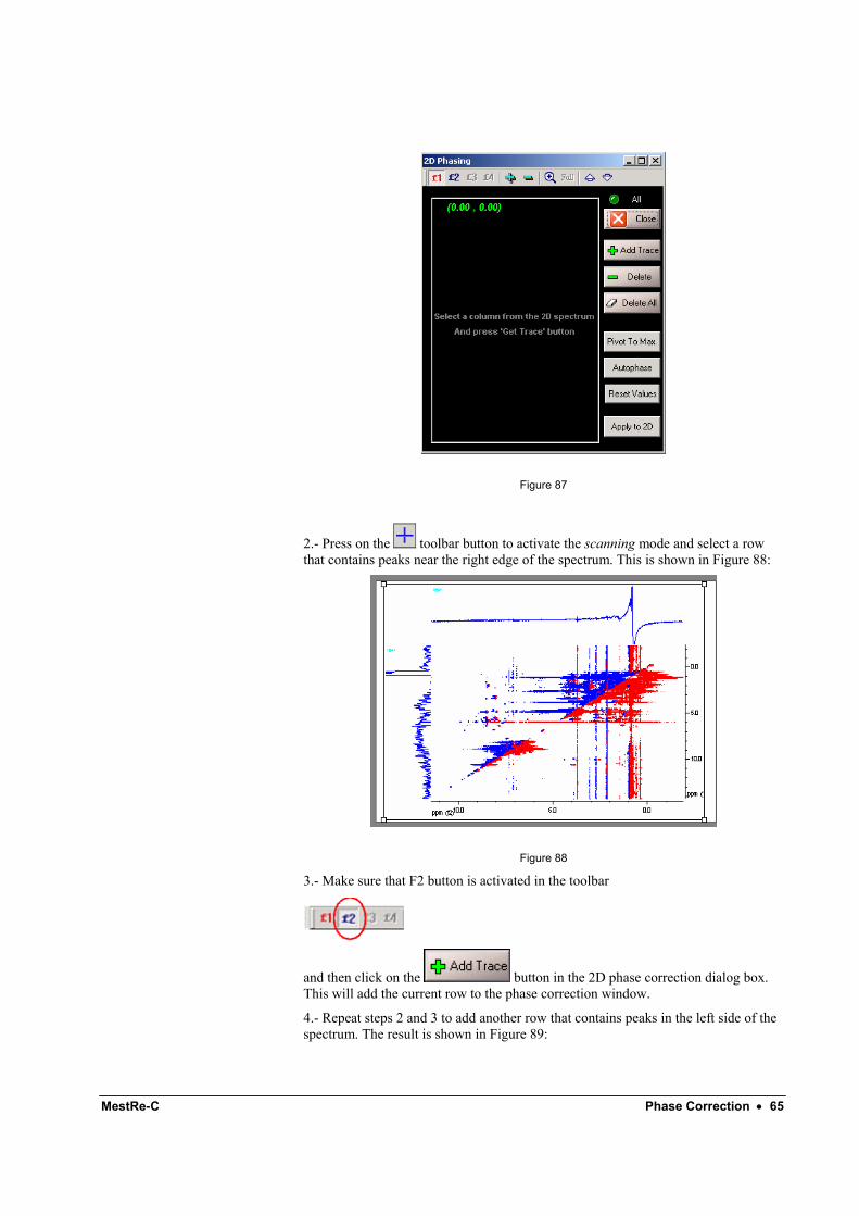
2D Phase Correction with individual traces Instead of performing the phase correction directly in the 2D full data matrix, with this method you can select a number of rows or columns (usually 2 or 3), correct the phase of those traces and, when satisfied, apply the correction to the full 2D spectrum.
As an example, we will show you how to correct the phase of the following TOCSY spectrum, where the blue colour indicates positive contours and red colour negative contours.
1.- Select command Process/Phase Correction/2D Phase Correction with 1D-Slices. You will get the following dialog box:
MestRe-C Phase Correction • 65
Figure 87
2.- Press on the toolbar button to activate the scanning mode and select a row that contains peaks near the right edge of the spectrum. This is shown in Figure 88:
Figure 88
3.- Make sure that F2 button is activated in the toolbar
and then click on the button in the 2D phase correction dialog box. This will add the current row to the phase correction window.
4.- Repeat steps 2 and 3 to add another row that contains peaks in the left side of the spectrum. The result is shown in Figure 89:
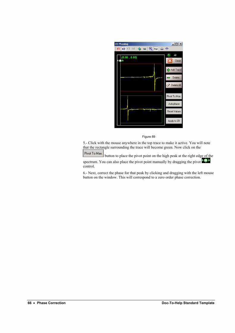
66 • Phase Correction Doc-To-Help Standard Template
Figure 89
5.- Click with the mouse anywhere in the top trace to make it active. You will note that the rectangle surrounding the trace will become green. Now click on the
button to place the pivot point on the high peak at the right edge of the spectrum. You can also place the pivot point manually by dragging the pivot control.
6.- Next, correct the phase for that peak by clicking and dragging with the left mouse button on the window. This will correspond to a zero order phase correction.
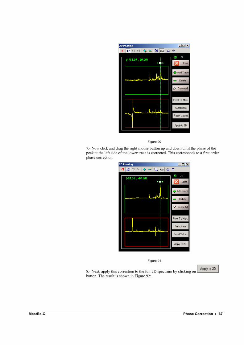
MestRe-C Phase Correction • 67
Figure 90
7.- Now click and drag the right mouse button up and down until the phase of the peak at the left side of the lower trace is corrected. This corresponds to a first order phase correction.
Figure 91
8.- Next, apply this correction to the full 2D spectrum by clicking on button. The result is shown in Figure 92:
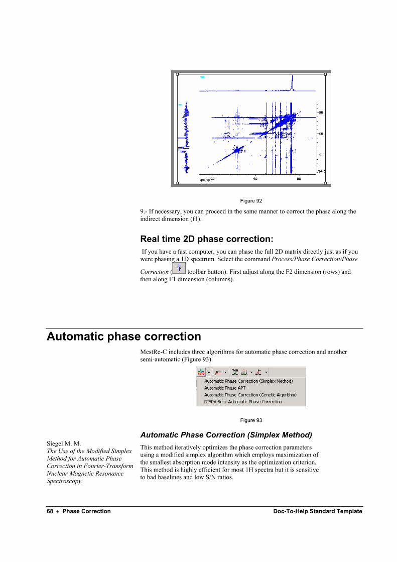
68 • Phase Correction Doc-To-Help Standard Template
Figure 92
9.- If necessary, you can proceed in the same manner to correct the phase along the indirect dimension (f1).
Real time 2D phase correction: If you have a fast computer, you can phase the full 2D matrix directly just as if you were phasing a 1D spectrum. Select the command Process/Phase Correction/Phase
Correction ( toolbar button). First adjust along the F2 dimension (rows) and then along F1 dimension (columns).
Automatic phase correction MestRe-C includes three algorithms for automatic phase correction and another semi-automatic (Figure 93).
Figure 93
Automatic Phase Correction (Simplex Method) Siegel M. M. The Use of the Modified Simplex Method for Automatic Phase Correction in Fourier-Transform Nuclear Magnetic Resonance Spectroscopy.
This method iteratively optimizes the phase correction parameters using a modified simplex algorithm which employs maximization of the smallest absorption mode intensity as the optimization criterion. This method is highly efficient for most 1H spectra but it is sensitive to bad baselines and low S/N ratios.

MestRe-C Phase Correction • 69
Anal. Chim. Acta, 1981, 133, 103-108.
Automatic Phase APT This method is a modification of the previous algorithm for the phase correction of APT and DEPT experiments, i.e. spectra with both positive and negative peaks. The program creates a list of the highest 10 peaks in the spectrum and then uses symmetrization criteria to find the optimal phasing parameters.
Automatic Phase-Correction (Genetic Algorithm) Li Chen,a Zhiqiang Weng, LaiYoong Goh, and Marc Garlandc.
An efficient algorithm for automatic phase correction of NMR spectra based on entropy minimization
J. Magn. Reson. 2002, 108, 164–168
This method uses a real-coded genetic algorithm to solve the optimization problem based on an entropy minimization.
DISPA Semi-Automatic Phase Correction Sotak C. H.; Dumoulin C. L.; Newsham M. D. Automatic Phase Correction of Fourier Transform NMR Spectra Based on the Dispersion versus Absorption (DISPA) Lineshape Analysis. J. Magn. Reson., 1984, 57, 453-462.
This method requires two well resolved lorentzian singlets. You will use the following dialog box to select the two lines.
Figure 94

MestRe-C Baseline/plane Correction • 71
Baseline/plane Correction
Introduction The baseline of a 1D spectrum is the theoretical line that connects the spectrum points which are neither peaks nor artefacts. When this baseline is not flat and/or it is offset from zero, a number of problems arise. First, the identification of peaks of interest may be more complicated. Also, when quantitative data must be extracted by integration, it is found that slight departures from a perfect baseline can cause considerable problems if quantification of the peak parameters is required (e.g. integration, peak fitting, etc).
2D spectra suffer from baseline problems which may cause difficulties in the visualization of the full data set at once, since the signals of interest may be smaller than the baseline distortions. specially for phase-sensitive experiments and when a large residual solvent signal distorts the baseline.
Thus, it turns out that baseline or baseplane correction is a very important processing step to obtain good quality spectra. MestRe-C includes two modules for baseline correction:
1. Polynomial baseline correction
2. Advanced baseline correction
Important: After applying a baseline/plane correction with MestRe-C, the imaginary part of the spectrum will be discarded. This means that if you want to adjust the phase afterwards, you will need to reconstruct the imaginary part through a Hilbert transform. Just press Ctrl+H and the spectrum will be complex again.
Polynomial baseline correction Dietrich W.; Rudel C. H.; Neumann M. Fast and Precise Automatic Baseline Correction of One- and Two-Dimensional NMR Spectra. J. Magn. Reson., 1991 91, 1-10.
This is a semi-automatic method in which the program finds automatically the baseline points (Dietrich et al) and then fits those points to a polynomial function (up to the seventh degree) or to a trigonometric series: F(x) = a(0) + a(1) cos(x) + b(1) sin(x) + a(2) cos(2x) + b(2) sin(2x) + … b(5) cos(5x).
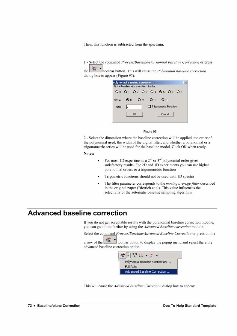
72 • Baseline/plane Correction Doc-To-Help Standard Template
Then, this function is subtracted from the spectrum.
1.- Select the command Process/Baseline/Polynomial Baseline Correction or press
the toolbar button. This will cause the Polynomial baseline correction dialog box to appear (Figure 95):
Figure 95
2.- Select the dimension where the baseline correction will be applied, the order of the polynomial used, the width of the digital filter, and whether a polynomial or a trigonometric series will be used for the baseline model. Click OK when ready.
Notes:
• For most 1D experiments a 2nd or 3rd polynomial order gives satisfactory results. For 2D and 3D experiments you can use higher polynomial orders or a trigonometric function
• Trigometric functions should not be used with 1D spectra
• The filter parameter corresponds to the moving average filter described in the original paper (Dietrich et al). This value influences the selectivity of the automatic baseline sampling algorithm.
Advanced baseline correction If you do not get acceptable results with the polynomial baseline correction module, you can go a little further by using the Advanced Baseline correction module.
Select the command Process/Baseline/Advanced Baseline Correction or press on the
arrow of the toolbar button to display the popup menu and select there the advanced baseline correction option:
This will cause the Advanced Baseline Correction dialog box to appear:
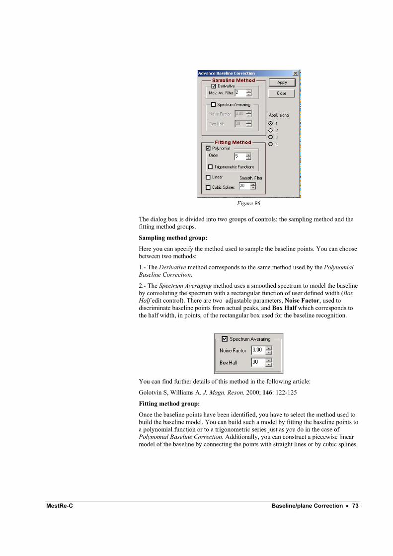
MestRe-C Baseline/plane Correction • 73
Figure 96
The dialog box is divided into two groups of controls: the sampling method and the fitting method groups.
Sampling method group:
Here you can specify the method used to sample the baseline points. You can choose between two methods:
1.- The Derivative method corresponds to the same method used by the Polynomial Baseline Correction.
2.- The Spectrum Averaging method uses a smoothed spectrum to model the baseline by convoluting the spectrum with a rectangular function of user defined width (Box Half edit control). There are two adjustable parameters, Noise Factor, used to discriminate baseline points from actual peaks, and Box Half which corresponds to the half width, in points, of the rectangular box used for the baseline recognition.
You can find further details of this method in the following article:
Golotvin S, Williams A. J. Magn. Reson. 2000; 146: 122-125
Fitting method group:
Once the baseline points have been identified, you have to select the method used to build the baseline model. You can build such a model by fitting the baseline points to a polynomial function or to a trigonometric series just as you do in the case of Polynomial Baseline Correction. Additionally, you can construct a piecewise linear model of the baseline by connecting the points with straight lines or by cubic splines.
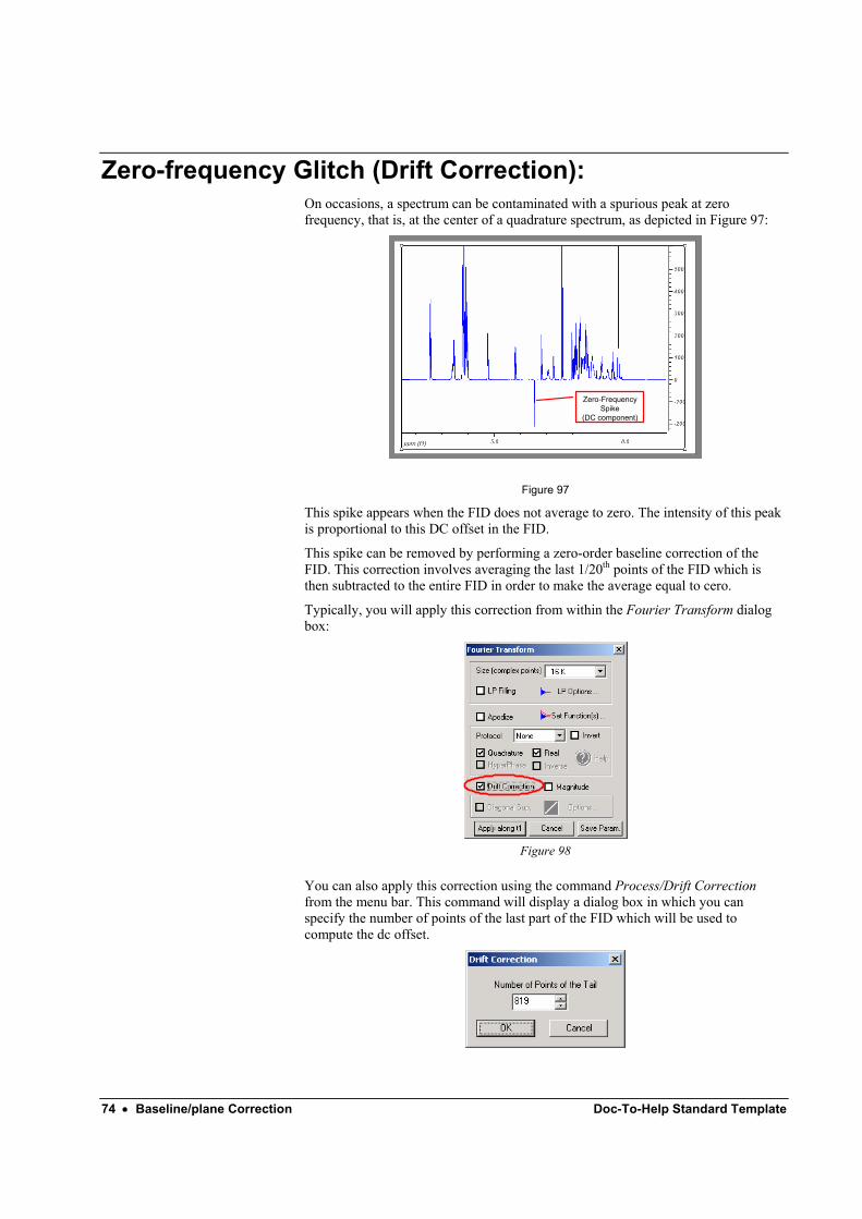
74 • Baseline/plane Correction Doc-To-Help Standard Template
Zero-frequency Glitch (Drift Correction): On occasions, a spectrum can be contaminated with a spurious peak at zero frequency, that is, at the center of a quadrature spectrum, as depicted in Figure 97:
Zero-Frequency Spike
(DC component)
Figure 97
This spike appears when the FID does not average to zero. The intensity of this peak is proportional to this DC offset in the FID.
This spike can be removed by performing a zero-order baseline correction of the FID. This correction involves averaging the last 1/20th points of the FID which is then subtracted to the entire FID in order to make the average equal to cero.
Typically, you will apply this correction from within the Fourier Transform dialog box:
Figure 98
You can also apply this correction using the command Process/Drift Correction from the menu bar. This command will display a dialog box in which you can specify the number of points of the last part of the FID which will be used to compute the dc offset.

MestRe-C Baseline/plane Correction • 75
This correction should be applied before apodizing the FID. It is disabled in nD spectra.

MestRe-C Integration • 77
Integration
Introduction Integration is the most frequently used method of NMR quantification. For example, integration of 1D NMR signals is typically used to estimate the number of species (e.g. protons) associated with a peak (or peaks) in the spectrum. Also, the volumes of crosspeaks in a NOESY (or ROESY) experiment are directly related to the distances between atoms in a molecule.
MestRe-C includes both 1D and 2D integration capabilities. Manual integration is the same in both 1- and 2-dimensional spectra
Integration values are measured as the sum of all digital intensities within user-defined boundaries. Therefore, it is usually advisable to increase the digital resolution by means of zero-filling or Linear Prediction. For example, in the case of 1D spectra, at least 4 or 5 digital points per full width at half height are recommended in order to minimize integration errors.
Besides, you should take into account that some apodization functions (e.g. Gaussian) can alter the integration values.
Finally, MestRe-C provides basic assignment facilities.
1D Integration Both manual and automatic integration routines are available.
Manual Integration To integrate the spectrum interactively, select the command
Tools/Integration/Integrate in the menu bar or click on the button in the toolbar and then press and drag the left mouse button to define a region around the peak(s) of interest (Figure 99).
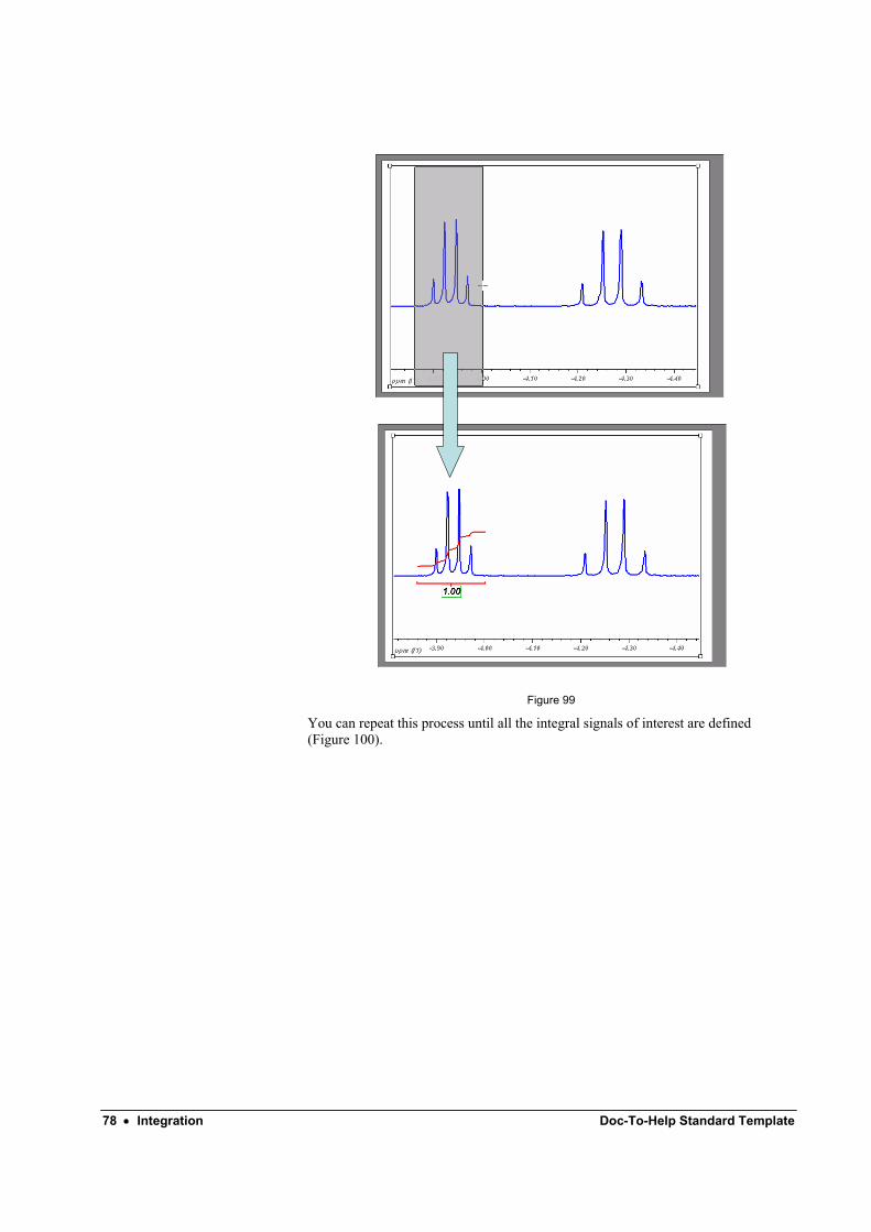
78 • Integration Doc-To-Help Standard Template
Figure 99
You can repeat this process until all the integral signals of interest are defined (Figure 100).
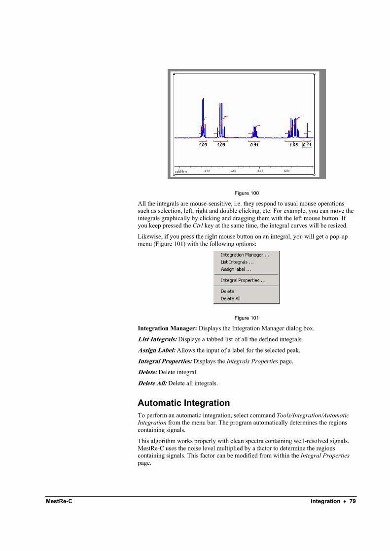
MestRe-C Integration • 79
Figure 100
All the integrals are mouse-sensitive, i.e. they respond to usual mouse operations such as selection, left, right and double clicking, etc. For example, you can move the integrals graphically by clicking and dragging them with the left mouse button. If you keep pressed the Ctrl key at the same time, the integral curves will be resized.
Likewise, if you press the right mouse button on an integral, you will get a pop-up menu (Figure 101) with the following options:
Figure 101
Integration Manager: Displays the Integration Manager dialog box.
List Integrals: Displays a tabbed list of all the defined integrals.
Assign Label: Allows the input of a label for the selected peak.
Integral Properties: Displays the Integrals Properties page.
Delete: Delete integral.
Delete All: Delete all integrals.
Automatic Integration To perform an automatic integration, select command Tools/Integration/Automatic Integration from the menu bar. The program automatically determines the regions containing signals.
This algorithm works properly with clean spectra containing well-resolved signals. MestRe-C uses the noise level multiplied by a factor to determine the regions containing signals. This factor can be modified from within the Integral Properties page.
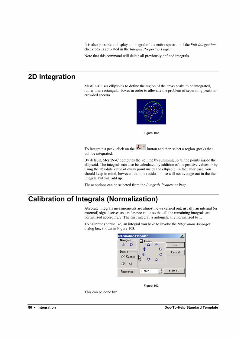
80 • Integration Doc-To-Help Standard Template
It is also possible to display an integral of the entire spectrum if the Full Integration check box is activated in the Integral Properties Page.
Note that this command will delete all previously defined integrals.
2D Integration MestRe-C uses ellipsoids to define the region of the cross peaks to be integrated, rather than rectangular boxes in order to alleviate the problem of separating peaks in crowded spectra.
Figure 102
To integrate a peak, click on the button and then select a region (peak) that will be integrated.
By default, MestRe-C computes the volume by summing up all the points inside the ellipsoid. The integrals can also be calculated by addition of the positive values or by using the absolute value of every point inside the ellipsoid. In the latter case, you should keep in mind, however, that the residual noise will not average out in the the integral, but will add up.
These options can be selected from the Integrals Properties Page.
Calibration of Integrals (Normalization) Absolute integrals measurements are almost never carried out; usually an internal (or external) signal serves as a reference value so that all the remaining integrals are normalized accordingly. The first integral is automatically normalized to 1.
To calibrate (normalize) an integral you have to invoke the Integration Manager dialog box shown in Figure 103:
Figure 103
This can be done by:
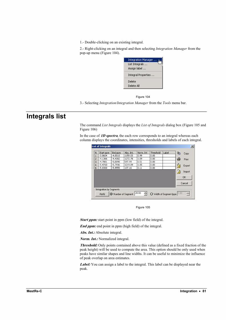
MestRe-C Integration • 81
1.- Double-clicking on an existing integral.
2.- Right-clicking on an integral and then selecting Integration Manager from the pop-up menu (Figure 104).
Figure 104
3.- Selecting Integration/Integration Manager from the Tools menu bar.
Integrals list The command List Integrals displays the List of Integrals dialog box (Figure 105 and Figure 106)
In the case of 1D spectra, the each row corresponds to an integral whereas each column displays the coordinates, intensities, thresholds and labels of each integral.
Figure 105
Start ppm: start point in ppm (low field) of the integral.
End ppm: end point in ppm (high field) of the integral.
Abs. Int.: Absolute integral.
Norm. Int.: Normalized integral.
Threshold: Only points contained above this value (defined as a fixed fraction of the peak height) will be used to compute the area. This option should be only used when peaks have similar shapes and line widths. It can be useful to minimize the influence of peak overlap on area estimates.
Label: You can assign a label to the integral. This label can be displayed near the peak.
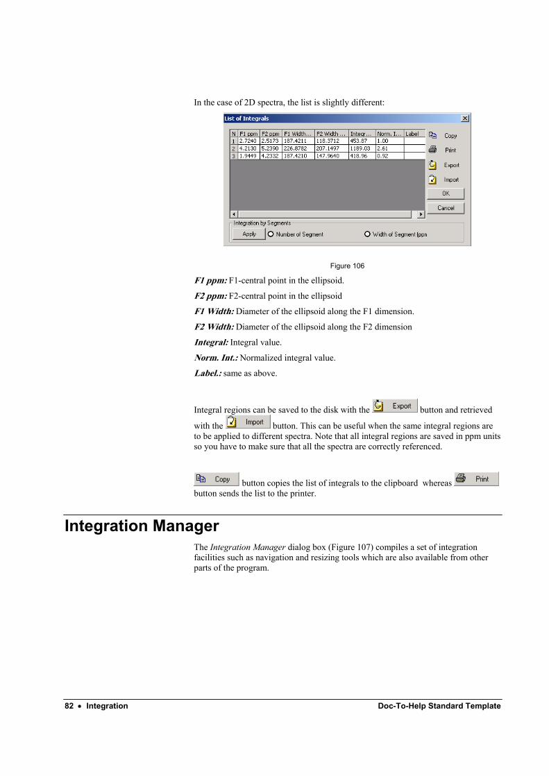
82 • Integration Doc-To-Help Standard Template
In the case of 2D spectra, the list is slightly different:
Figure 106
F1 ppm: F1-central point in the ellipsoid.
F2 ppm: F2-central point in the ellipsoid
F1 Width: Diameter of the ellipsoid along the F1 dimension.
F2 Width: Diameter of the ellipsoid along the F2 dimension
Integral: Integral value.
Norm. Int.: Normalized integral value.
Label.: same as above.
Integral regions can be saved to the disk with the button and retrieved
with the button. This can be useful when the same integral regions are to be applied to different spectra. Note that all integral regions are saved in ppm units so you have to make sure that all the spectra are correctly referenced.
button copies the list of integrals to the clipboard whereas button sends the list to the printer.
Integration Manager The Integration Manager dialog box (Figure 107) compiles a set of integration facilities such as navigation and resizing tools which are also available from other parts of the program.
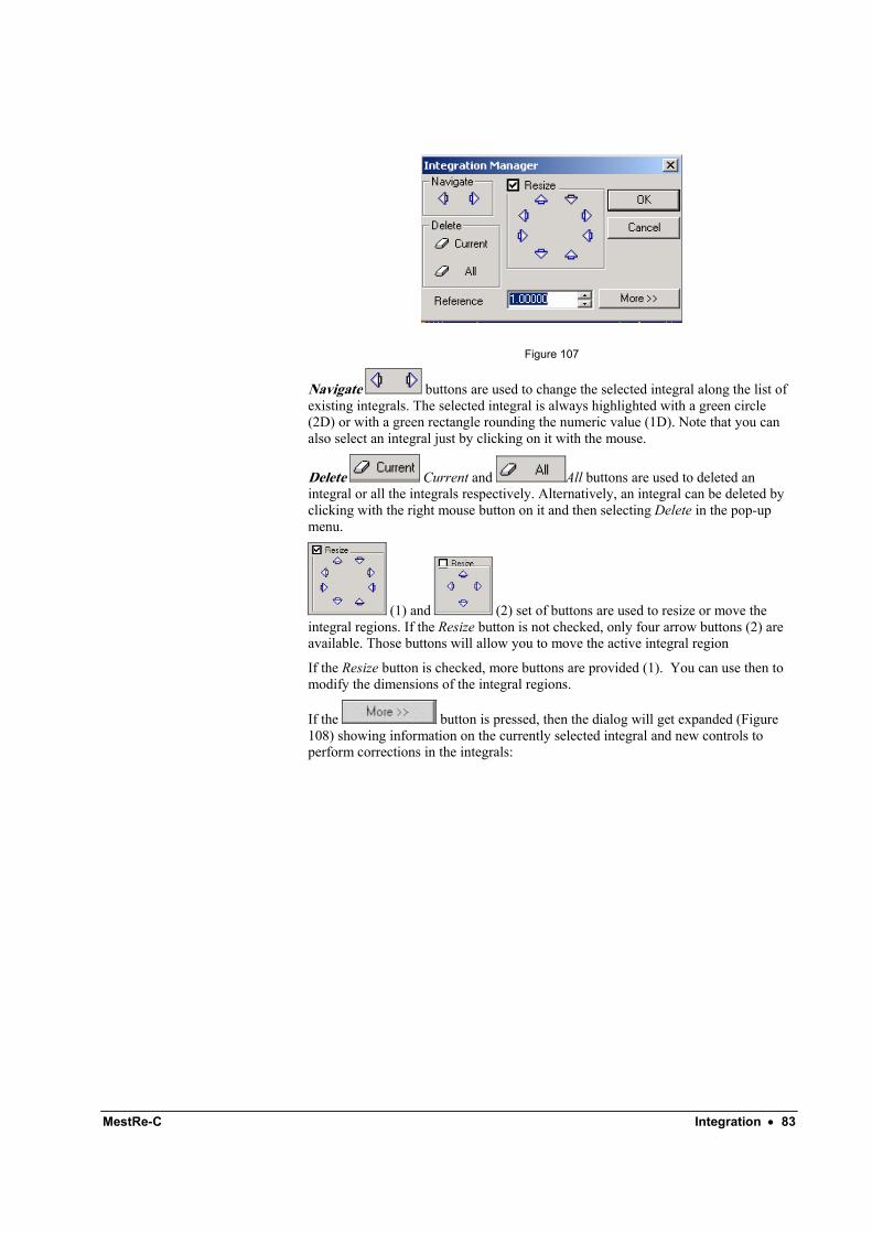
MestRe-C Integration • 83
Figure 107
Navigate buttons are used to change the selected integral along the list of existing integrals. The selected integral is always highlighted with a green circle (2D) or with a green rectangle rounding the numeric value (1D). Note that you can also select an integral just by clicking on it with the mouse.
Delete Current and All buttons are used to deleted an integral or all the integrals respectively. Alternatively, an integral can be deleted by clicking with the right mouse button on it and then selecting Delete in the pop-up menu.
(1) and (2) set of buttons are used to resize or move the integral regions. If the Resize button is not checked, only four arrow buttons (2) are available. Those buttons will allow you to move the active integral region
If the Resize button is checked, more buttons are provided (1). You can use then to modify the dimensions of the integral regions.
If the button is pressed, then the dialog will get expanded (Figure 108) showing information on the currently selected integral and new controls to perform corrections in the integrals:
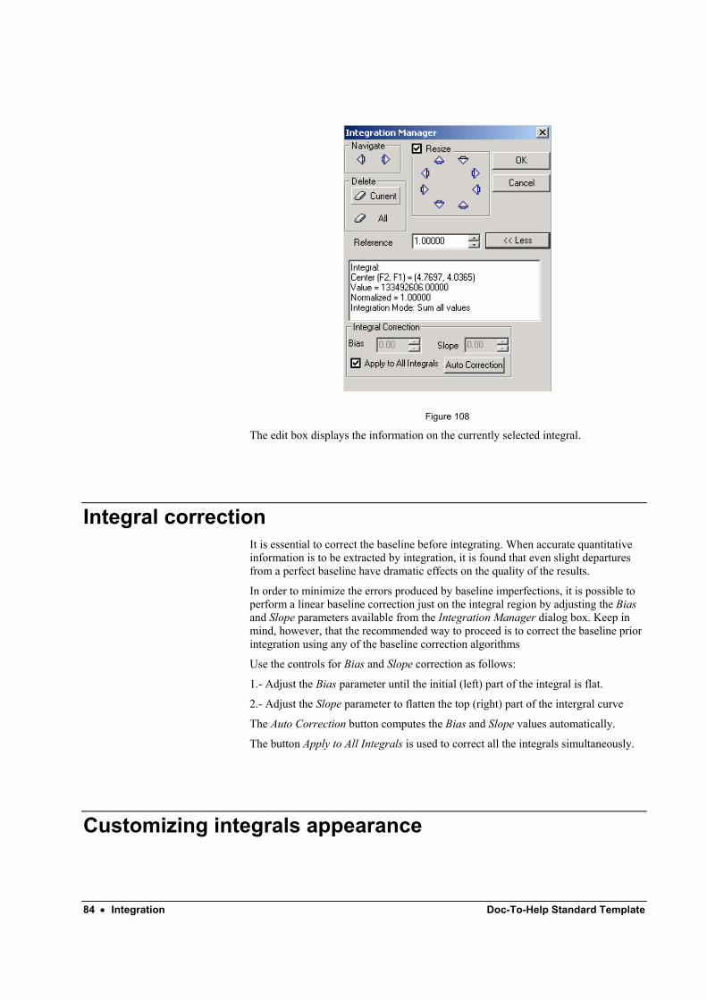
84 • Integration Doc-To-Help Standard Template
Figure 108
The edit box displays the information on the currently selected integral.
Integral correction It is essential to correct the baseline before integrating. When accurate quantitative information is to be extracted by integration, it is found that even slight departures from a perfect baseline have dramatic effects on the quality of the results.
In order to minimize the errors produced by baseline imperfections, it is possible to perform a linear baseline correction just on the integral region by adjusting the Bias and Slope parameters available from the Integration Manager dialog box. Keep in mind, however, that the recommended way to proceed is to correct the baseline prior integration using any of the baseline correction algorithms
Use the controls for Bias and Slope correction as follows:
1.- Adjust the Bias parameter until the initial (left) part of the integral is flat.
2.- Adjust the Slope parameter to flatten the top (right) part of the intergral curve
The Auto Correction button computes the Bias and Slope values automatically.
The button Apply to All Integrals is used to correct all the integrals simultaneously.
Customizing integrals appearance
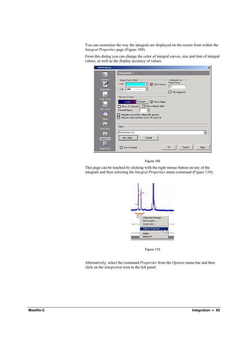
MestRe-C Integration • 85
You can customize the way the integrals are displayed on the screen from within the Integral Properties page (Figure 109).
From this dialog you can change the color of integral curves, size and font of integral values, as well as the display accuracy of values.
Figure 109
This page can be reached by clicking with the right mouse button on any of the integrals and then selecting the Integral Properties menu command (Figure 110):
Figure 110
Alternatively, select the command Properties from the Options menu bar and then click on the Integration icon in the left panel.

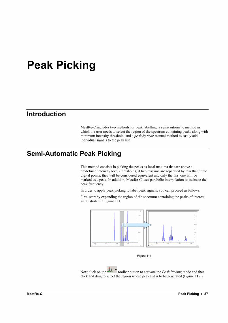
MestRe-C Peak Picking • 87
Peak Picking
Introduction
MestRe-C includes two methods for peak labelling: a semi-automatic method in which the user needs to select the region of the spectrum containing peaks along with minimum intensity threshold, and a peak by peak manual method to easily add individual signals to the peak list.
Semi-Automatic Peak Picking
This method consists in picking the peaks as local maxima that are above a predefined intensity level (threshold); if two maxima are separated by less than three digital points, they will be considered equivalent and only the first one will be marked as a peak. In addition, MestRe-C uses parabolic interpolation to estimate the peak frequency.
In order to apply peak picking to label peak signals, you can proceed as follows:
First, start by expanding the region of the spectrum containing the peaks of interest as illustrated in Figure 111.
Figure 111
Next click on the toolbar button to activate the Peak Picking mode and then click and drag to select the region whose peak list is to be generated (Figure 112.).
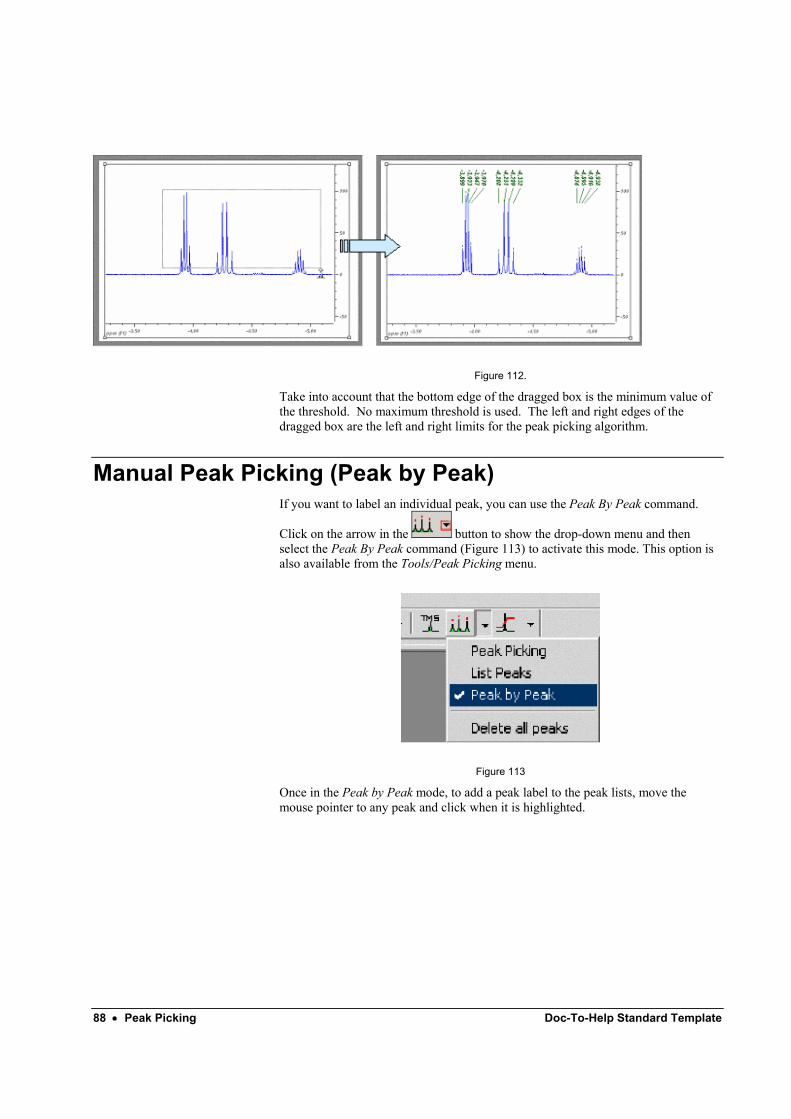
88 • Peak Picking Doc-To-Help Standard Template
Figure 112.
Take into account that the bottom edge of the dragged box is the minimum value of the threshold. No maximum threshold is used. The left and right edges of the dragged box are the left and right limits for the peak picking algorithm.
Manual Peak Picking (Peak by Peak) If you want to label an individual peak, you can use the Peak By Peak command.
Click on the arrow in the button to show the drop-down menu and then select the Peak By Peak command (Figure 113) to activate this mode. This option is also available from the Tools/Peak Picking menu.
Figure 113
Once in the Peak by Peak mode, to add a peak label to the peak lists, move the mouse pointer to any peak and click when it is highlighted.
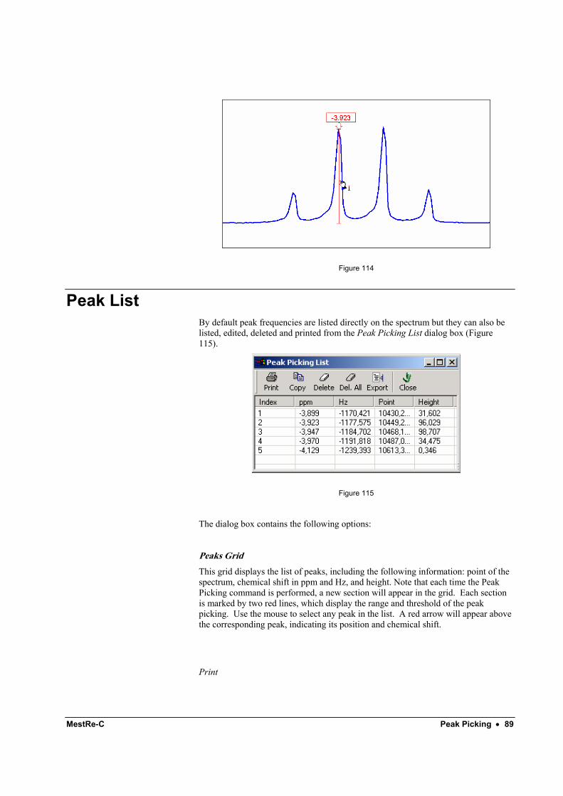
MestRe-C Peak Picking • 89
Figure 114
Peak List By default peak frequencies are listed directly on the spectrum but they can also be listed, edited, deleted and printed from the Peak Picking List dialog box (Figure 115).
Figure 115
The dialog box contains the following options:
Peaks Grid This grid displays the list of peaks, including the following information: point of the spectrum, chemical shift in ppm and Hz, and height. Note that each time the Peak Picking command is performed, a new section will appear in the grid. Each section is marked by two red lines, which display the range and threshold of the peak picking. Use the mouse to select any peak in the list. A red arrow will appear above the corresponding peak, indicating its position and chemical shift.

90 • Peak Picking Doc-To-Help Standard Template
Click this button to print the list of chemical shifts.
Customize
Click this button to customize the layout of the peak picking list. A new dialog box will be opened. Click Print to close the dialog box; click Printer Setup to display the Print Setup Dialog Box or click Cancel at any time to exit the dialog box.
Headers and fonts
This section allows you to customize three sections for the peak picking print out: header, content and footer. The combo boxes are provided for changing the font type and font size for each section. The text boxes allow you to type an optional text for each section.
Tip: Use the %d to include the number of the page in the text of the section. Type the sequence CTRL+ENTER to include a carriage return in the text.
Margins
This section allows you to change the margins of print out.
Print Grid
If checked the grid is printed with border lines.
Copy
Click this button to copy the current peak picking list to the clipboard. Use this option to copy the list into any application using the corresponding Paste command.
Delete
Click this button to delete the currently selected peak from the list. If the last peak of that section is deleted, the entire section will disappear.

MestRe-C Peak Picking • 91
Delete All
Click this button to delete all the peaks on the list.
Export
Click this button to export the list of peaks to the clipboard as a line of values separated by commas or decimal points. To change the format of the exported peak picking, use the Export Options command included in the Options submenu.
Close
Click this button to close the dialog box and exit the command.

MestRe-C Analysis of arrayed experiments • 93
Analysis of arrayed experiments
Introduction MestRe-C includes a general-purpose fitting module designed to analyze arrayed experiments such as relaxation, kinetics or DOSY experiments using a robust but intuitive working environment. Within this module it is possible to employ several methods for extraction of data information from the NMR experiments, to inspect graphically the curve data for both the experimental and calculated data points and to perform the corresponding data fitting via non linear and polynomial fitting.
As an example, we will show you how to compute the diffusion coefficient of the methyl group of ethanol in a mixture of water/sucrose/ethanol. Keep in mind that you can follow the same procedure to calculate relaxation times or to analyze kinetic experiments.
Analysis of a DOSY experiment
After importing the experimental data set you will get a pseudo 2D experiment containing a series of diffusion weighted spectra.
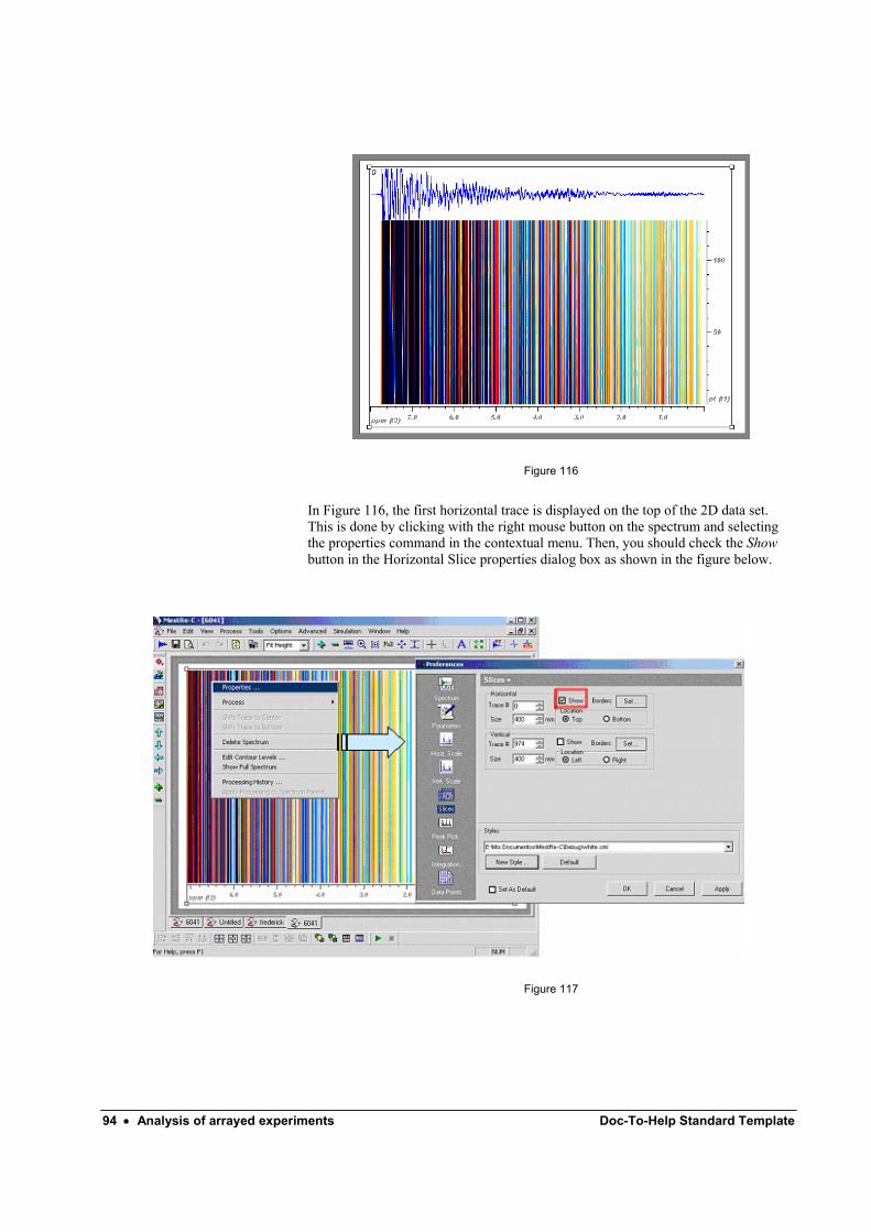
94 • Analysis of arrayed experiments Doc-To-Help Standard Template
Figure 116
In Figure 116, the first horizontal trace is displayed on the top of the 2D data set. This is done by clicking with the right mouse button on the spectrum and selecting the properties command in the contextual menu. Then, you should check the Show button in the Horizontal Slice properties dialog box as shown in the figure below.
Figure 117
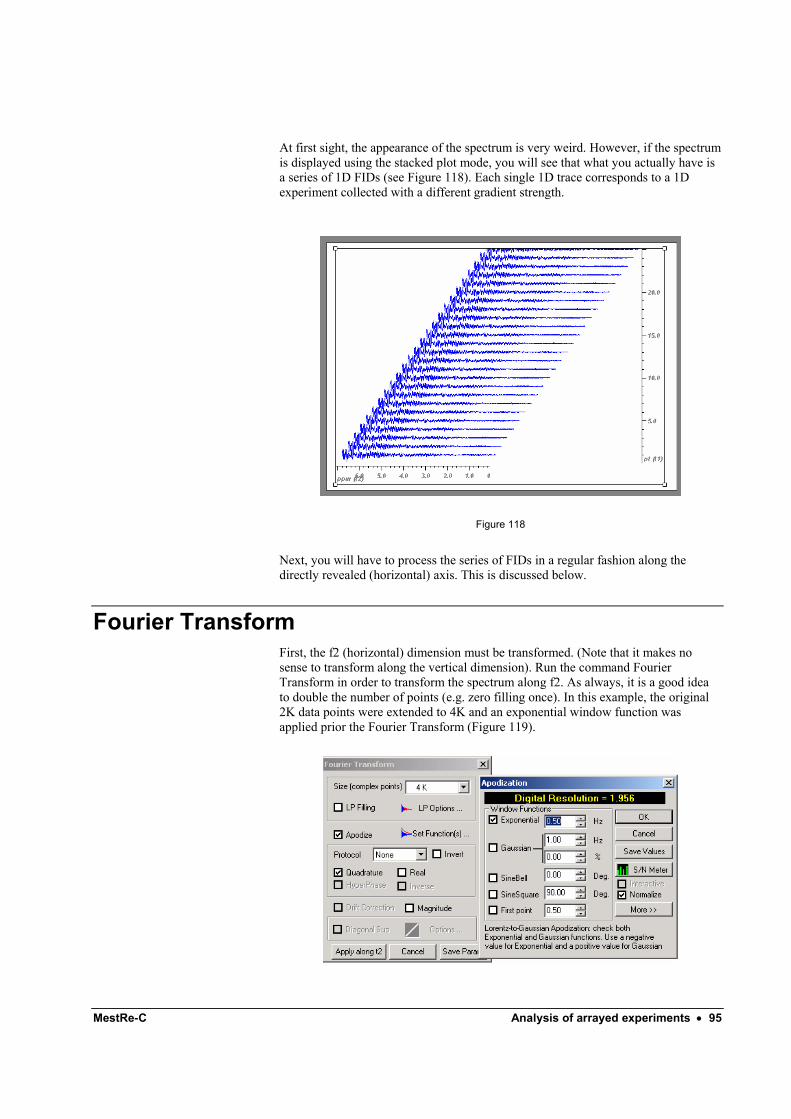
MestRe-C Analysis of arrayed experiments • 95
At first sight, the appearance of the spectrum is very weird. However, if the spectrum is displayed using the stacked plot mode, you will see that what you actually have is a series of 1D FIDs (see Figure 118). Each single 1D trace corresponds to a 1D experiment collected with a different gradient strength.
Figure 118
Next, you will have to process the series of FIDs in a regular fashion along the directly revealed (horizontal) axis. This is discussed below.
Fourier Transform First, the f2 (horizontal) dimension must be transformed. (Note that it makes no sense to transform along the vertical dimension). Run the command Fourier Transform in order to transform the spectrum along f2. As always, it is a good idea to double the number of points (e.g. zero filling once). In this example, the original 2K data points were extended to 4K and an exponential window function was applied prior the Fourier Transform (Figure 119).
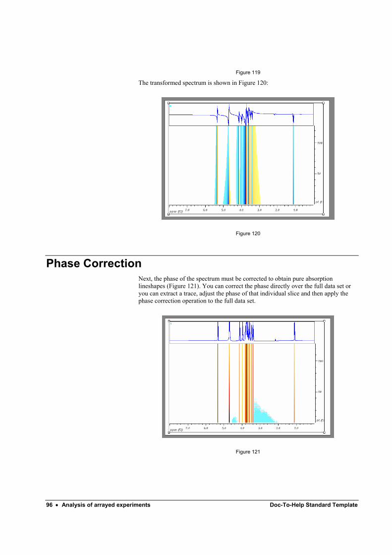
96 • Analysis of arrayed experiments Doc-To-Help Standard Template
Figure 119
The transformed spectrum is shown in Figure 120:
Figure 120
Phase Correction Next, the phase of the spectrum must be corrected to obtain pure absorption lineshapes (Figure 121). You can correct the phase directly over the full data set or you can extract a trace, adjust the phase of that individual slice and then apply the phase correction operation to the full data set.
Figure 121
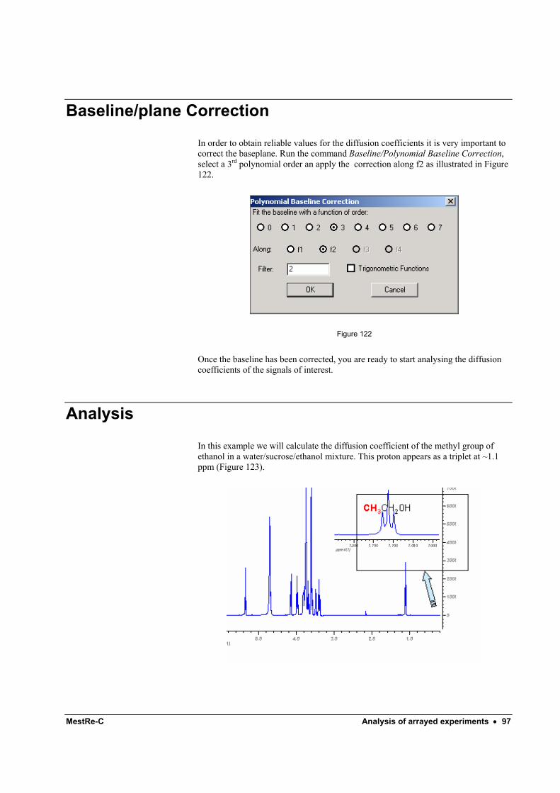
MestRe-C Analysis of arrayed experiments • 97
Baseline/plane Correction
In order to obtain reliable values for the diffusion coefficients it is very important to correct the baseplane. Run the command Baseline/Polynomial Baseline Correction, select a 3rd polynomial order an apply the correction along f2 as illustrated in Figure 122.
Figure 122
Once the baseline has been corrected, you are ready to start analysing the diffusion coefficients of the signals of interest.
Analysis
In this example we will calculate the diffusion coefficient of the methyl group of ethanol in a water/sucrose/ethanol mixture. This proton appears as a triplet at ~1.1 ppm (Figure 123).
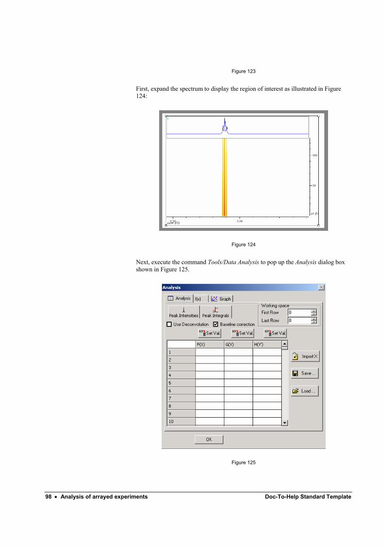
98 • Analysis of arrayed experiments Doc-To-Help Standard Template
Figure 123
First, expand the spectrum to display the region of interest as illustrated in Figure 124:
Figure 124
Next, execute the command Tools/Data Analysis to pop up the Analysis dialog box shown in Figure 125.
Figure 125
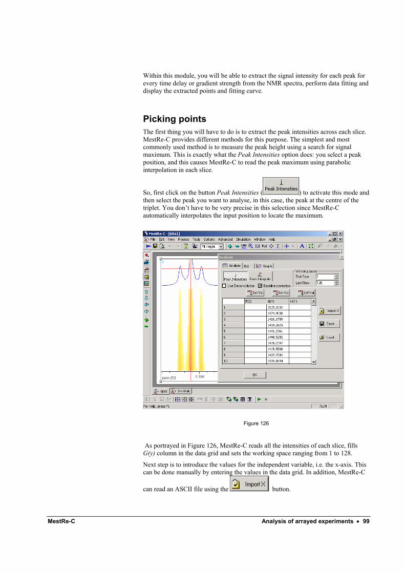
MestRe-C Analysis of arrayed experiments • 99
Within this module, you will be able to extract the signal intensity for each peak for every time delay or gradient strength from the NMR spectra, perform data fitting and display the extracted points and fitting curve.
Picking points The first thing you will have to do is to extract the peak intensities across each slice. MestRe-C provides different methods for this purpose. The simplest and most commonly used method is to measure the peak height using a search for signal maximum. This is exactly what the Peak Intensities option does: you select a peak position, and this causes MestRe-C to read the peak maximum using parabolic interpolation in each slice.
So, first click on the button Peak Intensities ( ) to activate this mode and then select the peak you want to analyse, in this case, the peak at the centre of the triplet. You don’t have to be very precise in this selection since MestRe-C automatically interpolates the input position to locate the maximum.
Figure 126
As portrayed in Figure 126, MestRe-C reads all the intensities of each slice, fills G(y) column in the data grid and sets the working space ranging from 1 to 128.
Next step is to introduce the values for the independent variable, i.e. the x-axis. This can be done manually by entering the values in the data grid. In addition, MestRe-C
can read an ASCII file using the button.
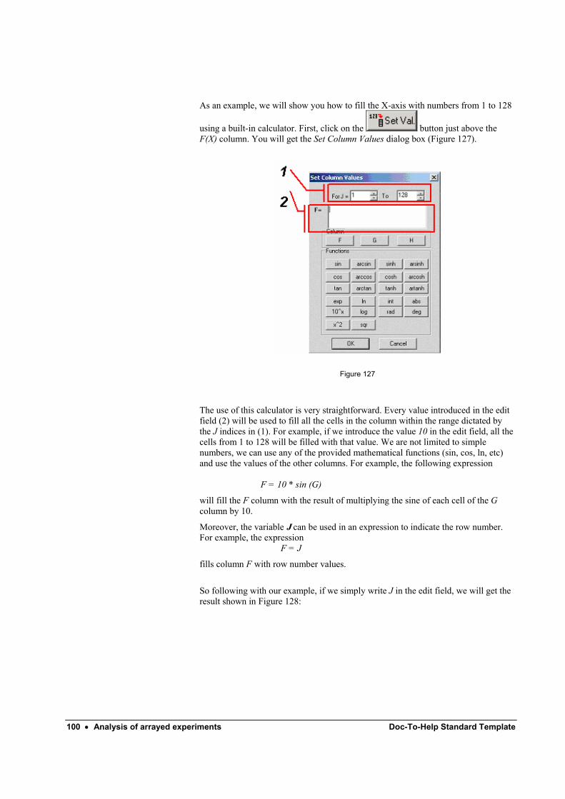
100 • Analysis of arrayed experiments Doc-To-Help Standard Template
As an example, we will show you how to fill the X-axis with numbers from 1 to 128
using a built-in calculator. First, click on the button just above the F(X) column. You will get the Set Column Values dialog box (Figure 127).
Figure 127
The use of this calculator is very straightforward. Every value introduced in the edit field (2) will be used to fill all the cells in the column within the range dictated by the J indices in (1). For example, if we introduce the value 10 in the edit field, all the cells from 1 to 128 will be filled with that value. We are not limited to simple numbers, we can use any of the provided mathematical functions (sin, cos, ln, etc) and use the values of the other columns. For example, the following expression
F = 10 * sin (G)
will fill the F column with the result of multiplying the sine of each cell of the G column by 10.
Moreover, the variable J can be used in an expression to indicate the row number. For example, the expression
F = J
fills column F with row number values.
So following with our example, if we simply write J in the edit field, we will get the result shown in Figure 128:
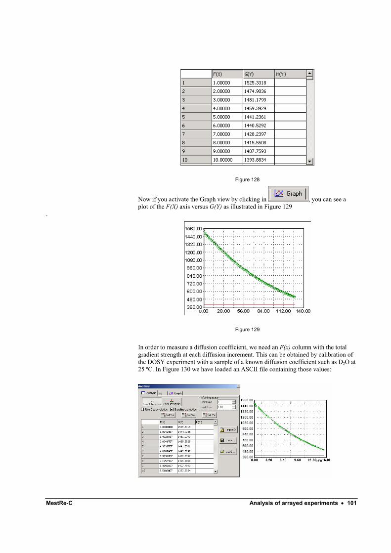
MestRe-C Analysis of arrayed experiments • 101
Figure 128
Now if you activate the Graph view by clicking in , you can see a plot of the F(X) axis versus G(Y) as illustrated in Figure 129
.
Figure 129
In order to measure a diffusion coefficient, we need an F(x) column with the total gradient strength at each diffusion increment. This can be obtained by calibration of the DOSY experiment with a sample of a known diffusion coefficient such as D2O at 25 ºC. In Figure 130 we have loaded an ASCII file containing those values:
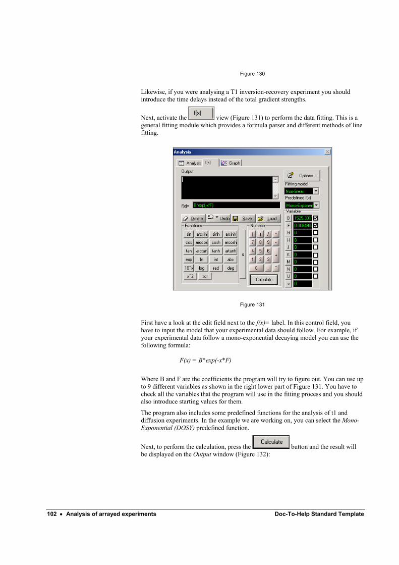
102 • Analysis of arrayed experiments Doc-To-Help Standard Template
Figure 130
Likewise, if you were analysing a T1 inversion-recovery experiment you should introduce the time delays instead of the total gradient strengths.
Next, activate the view (Figure 131) to perform the data fitting. This is a general fitting module which provides a formula parser and different methods of line fitting.
Figure 131
First have a look at the edit field next to the f(x)= label. In this control field, you have to input the model that your experimental data should follow. For example, if your experimental data follow a mono-exponential decaying model you can use the following formula:
F(x) = B*exp(-x*F)
Where B and F are the coefficients the program will try to figure out. You can use up to 9 different variables as shown in the right lower part of Figure 131. You have to check all the variables that the program will use in the fitting process and you should also introduce starting values for them.
The program also includes some predefined functions for the analysis of t1 and diffusion experiments. In the example we are working on, you can select the Mono-Exponential (DOSY) predefined function.
Next, to perform the calculation, press the button and the result will be displayed on the Output window (Figure 132):
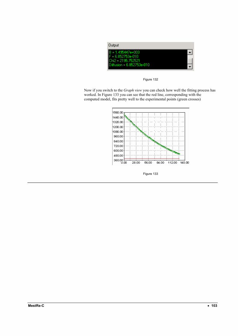
MestRe-C • 103
Figure 132
Now if you switch to the Graph view you can check how well the fitting process has worked. In Figure 133 you can see that the red line, corresponding with the computed model, fits pretty well to the experimental points (green crosses)
Figure 133

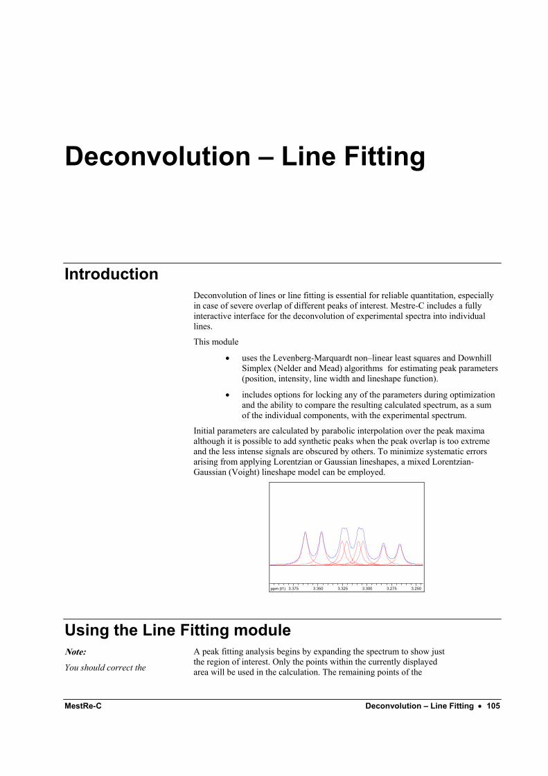
MestRe-C Deconvolution – Line Fitting • 105
Deconvolution – Line Fitting
Introduction Deconvolution of lines or line fitting is essential for reliable quantitation, especially in case of severe overlap of different peaks of interest. Mestre-C includes a fully interactive interface for the deconvolution of experimental spectra into individual lines.
This module
• uses the Levenberg-Marquardt non–linear least squares and Downhill Simplex (Nelder and Mead) algorithms for estimating peak parameters (position, intensity, line width and lineshape function).
• includes options for locking any of the parameters during optimization and the ability to compare the resulting calculated spectrum, as a sum of the individual components, with the experimental spectrum.
Initial parameters are calculated by parabolic interpolation over the peak maxima although it is possible to add synthetic peaks when the peak overlap is too extreme and the less intense signals are obscured by others. To minimize systematic errors arising from applying Lorentzian or Gaussian lineshapes, a mixed Lorentzian-Gaussian (Voight) lineshape model can be employed.
ppm (t1) 3.250 3.275 3.3003.3253.3503.375
Using the Line Fitting module Note:
You should correct the
A peak fitting analysis begins by expanding the spectrum to show just the region of interest. Only the points within the currently displayed area will be used in the calculation. The remaining points of the
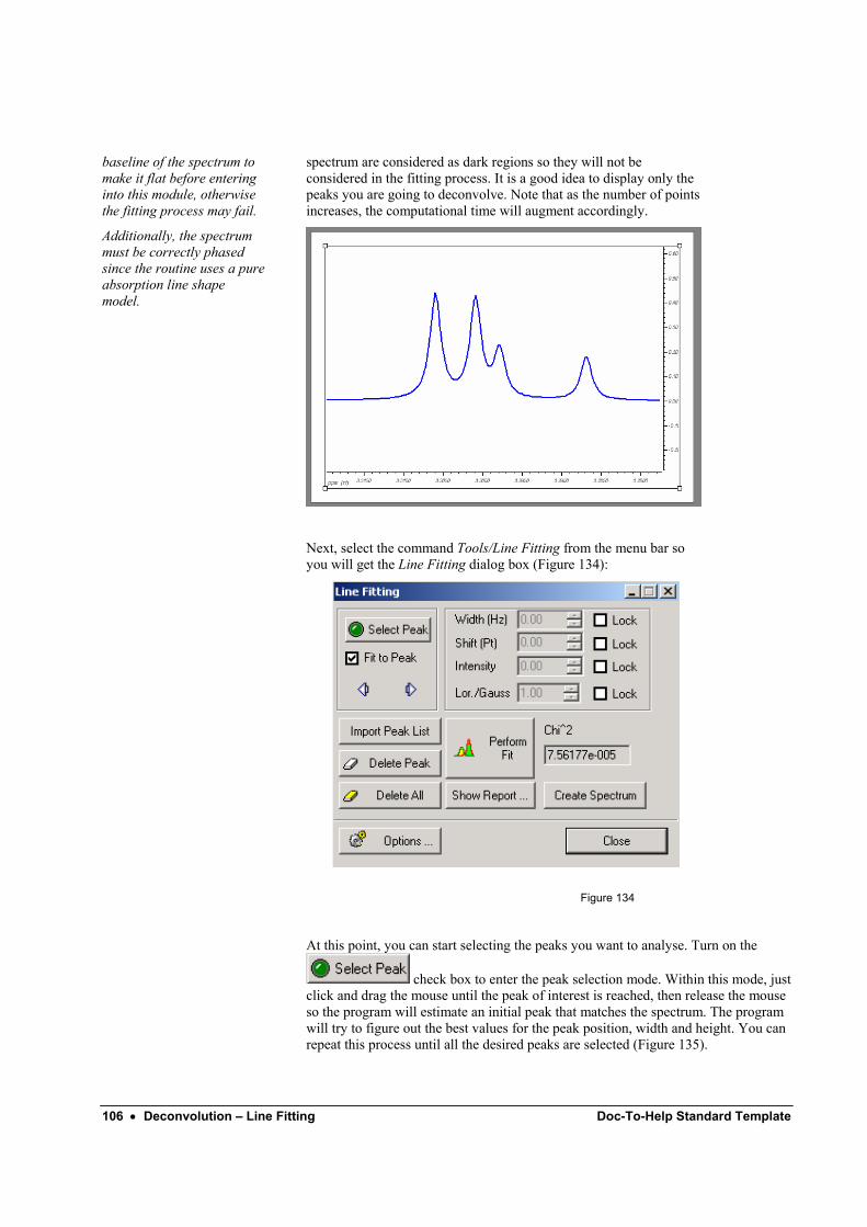
106 • Deconvolution – Line Fitting Doc-To-Help Standard Template
baseline of the spectrum to make it flat before entering into this module, otherwise the fitting process may fail.
Additionally, the spectrum must be correctly phased since the routine uses a pure absorption line shape model.
spectrum are considered as dark regions so they will not be considered in the fitting process. It is a good idea to display only the peaks you are going to deconvolve. Note that as the number of points increases, the computational time will augment accordingly.
Next, select the command Tools/Line Fitting from the menu bar so you will get the Line Fitting dialog box (Figure 134):
Figure 134
At this point, you can start selecting the peaks you want to analyse. Turn on the
check box to enter the peak selection mode. Within this mode, just click and drag the mouse until the peak of interest is reached, then release the mouse so the program will estimate an initial peak that matches the spectrum. The program will try to figure out the best values for the peak position, width and height. You can repeat this process until all the desired peaks are selected (Figure 135).
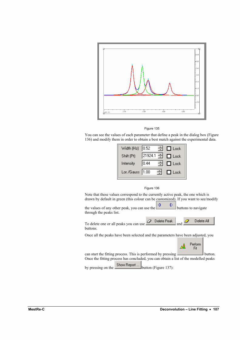
MestRe-C Deconvolution – Line Fitting • 107
Figure 135
You can see the values of each parameter that define a peak in the dialog box (Figure 136) and modify them in order to obtain a best match against the experimental data.
Figure 136
Note that these values correspond to the currently active peak, the one which is drawn by default in green (this colour can be customized). If you want to see/modify
the values of any other peak, you can use the buttons to navigate through the peaks list.
To delete one or all peaks you can use and buttons.
Once all the peaks have been selected and the parameters have been adjusted, you
can start the fitting process. This is performed by pressing button. Once the fitting process has concluded, you can obtain a list of the modelled peaks
by pressing on the button (Figure 137):
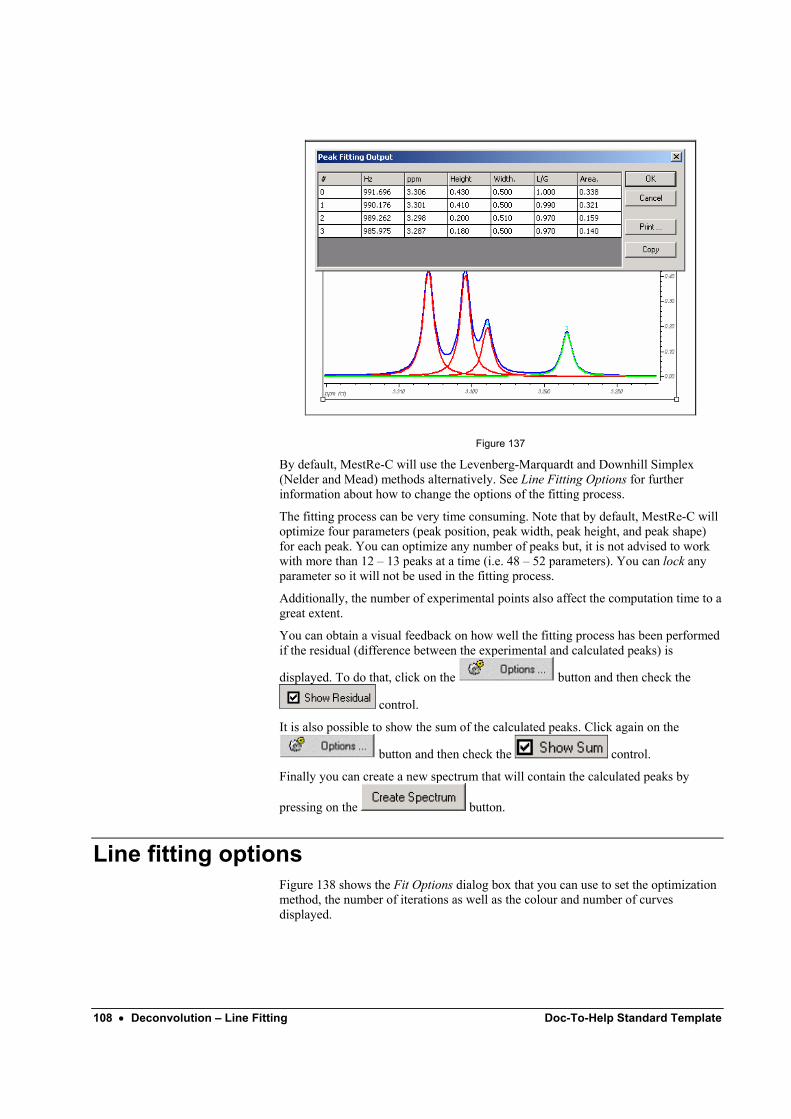
108 • Deconvolution – Line Fitting Doc-To-Help Standard Template
Figure 137
By default, MestRe-C will use the Levenberg-Marquardt and Downhill Simplex (Nelder and Mead) methods alternatively. See Line Fitting Options for further information about how to change the options of the fitting process.
The fitting process can be very time consuming. Note that by default, MestRe-C will optimize four parameters (peak position, peak width, peak height, and peak shape) for each peak. You can optimize any number of peaks but, it is not advised to work with more than 12 – 13 peaks at a time (i.e. 48 – 52 parameters). You can lock any parameter so it will not be used in the fitting process.
Additionally, the number of experimental points also affect the computation time to a great extent.
You can obtain a visual feedback on how well the fitting process has been performed if the residual (difference between the experimental and calculated peaks) is
displayed. To do that, click on the button and then check the
control.
It is also possible to show the sum of the calculated peaks. Click again on the
button and then check the control.
Finally you can create a new spectrum that will contain the calculated peaks by
pressing on the button.
Line fitting options Figure 138 shows the Fit Options dialog box that you can use to set the optimization method, the number of iterations as well as the colour and number of curves displayed.
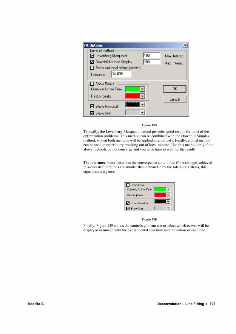
MestRe-C Deconvolution – Line Fitting • 109
Figure 138
Typically, the Levenberg-Marquadt method provides good results for most of the optimization problems. This method can be combined with the Downhill Simplex method, so that both methods will be applied alternatively. Finally, a third method can be used in order to try breaking out of local minima. Use this method only if the above methods do not converge and you have time to wait for the result!.
The tolerance factor describes the convergence conditions: if the changes achieved in successive iterations are smaller than demanded by the tolerance criteria, this signals convergence.
Figure 139
Finally, Figure 139 shows the controls you can use to select which curves will be displayed in unison with the experimental spectrum and the colour of each one.

MestRe-C Opening multiple spectra • 111
Opening multiple spectra
Introduction This section explains how to import and process multiple spectra simultaneously.
Importing multiple spectra
Adding files one-by-one You should start by selecting the command File/Import Multiple Spectra from the menu bar. You will get the following dialog box:
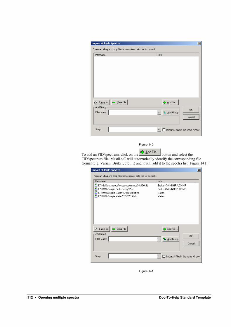
112 • Opening multiple spectra Doc-To-Help Standard Template
Figure 140
To add an FID/spectrum, click on the button and select the FID/spectrum file. MestRe-C will automatically identify the corresponding file format (e.g. Varian, Bruker, etc …) and it will add it to the spectra list (Figure 141):
Figure 141

MestRe-C Opening multiple spectra • 113
You can also add files to this list by just dragging the file from the windows explorer to the spectrum list control.
You can use and buttons to delete any or all the spectra files.
When you have finished selecting all the files, press the button so that MestRe-C will attempt to import all the spectra. Depending whether the
control is checked or not, all the files will be opened into different (Figure 142) or into the same window (Figure 143):
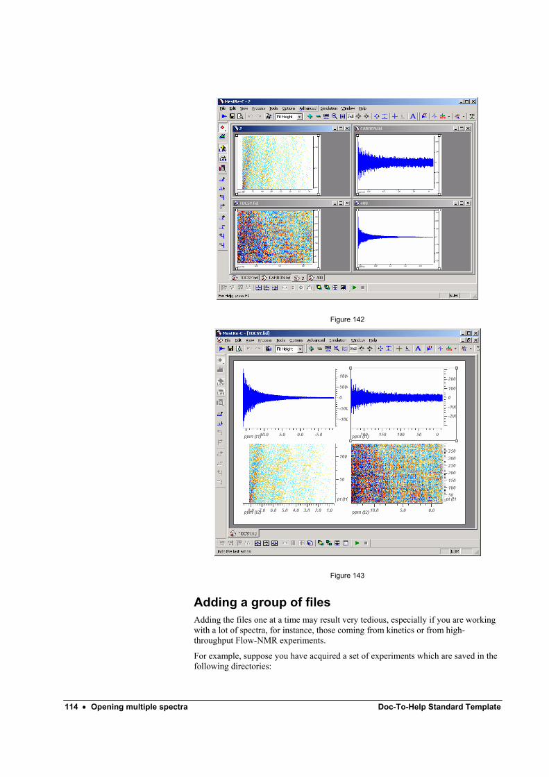
114 • Opening multiple spectra Doc-To-Help Standard Template
Figure 142
Figure 143
Adding a group of files Adding the files one at a time may result very tedious, especially if you are working with a lot of spectra, for instance, those coming from kinetics or from high-throughput Flow-NMR experiments.
For example, suppose you have acquired a set of experiments which are saved in the following directories:
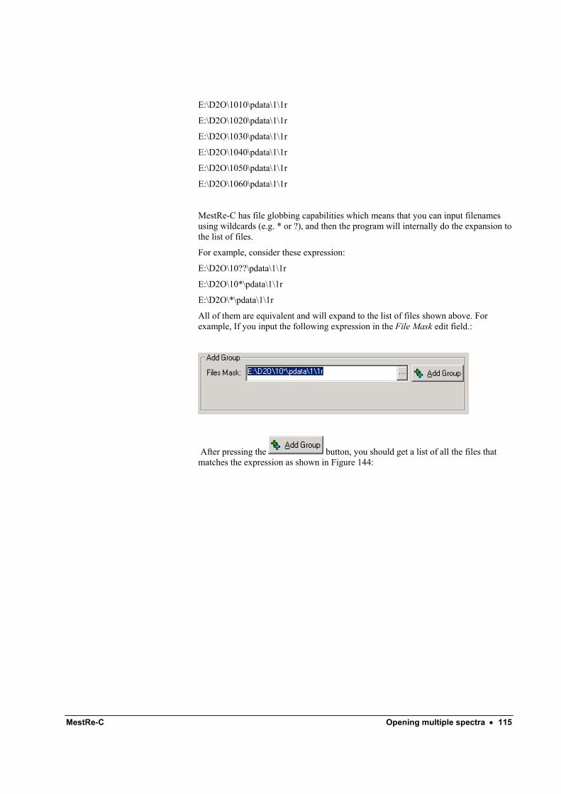
MestRe-C Opening multiple spectra • 115
E:\D2O\1010\pdata\1\1r
E:\D2O\1020\pdata\1\1r
E:\D2O\1030\pdata\1\1r
E:\D2O\1040\pdata\1\1r
E:\D2O\1050\pdata\1\1r
E:\D2O\1060\pdata\1\1r
MestRe-C has file globbing capabilities which means that you can input filenames using wildcards (e.g. * or ?), and then the program will internally do the expansion to the list of files.
For example, consider these expression:
E:\D2O\10??\pdata\1\1r
E:\D2O\10*\pdata\1\1r
E:\D2O\*\pdata\1\1r
All of them are equivalent and will expand to the list of files shown above. For example, If you input the following expression in the File Mask edit field.:
After pressing the button, you should get a list of all the files that matches the expression as shown in Figure 144:
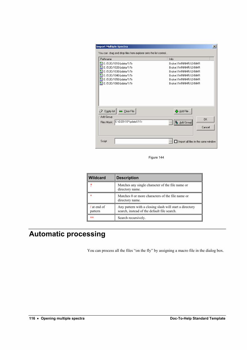
116 • Opening multiple spectra Doc-To-Help Standard Template
Figure 144
Wildcard Description ? Matches any single character of the file name or
directory name.
* Matches 0 or more characters of the file name or directory name.
/ at end of pattern
Any pattern with a closing slash will start a directory search, instead of the default file search.
** Search recursively.
Automatic processing
You can process all the files “on the fly” by assigning a macro file in the dialog box.
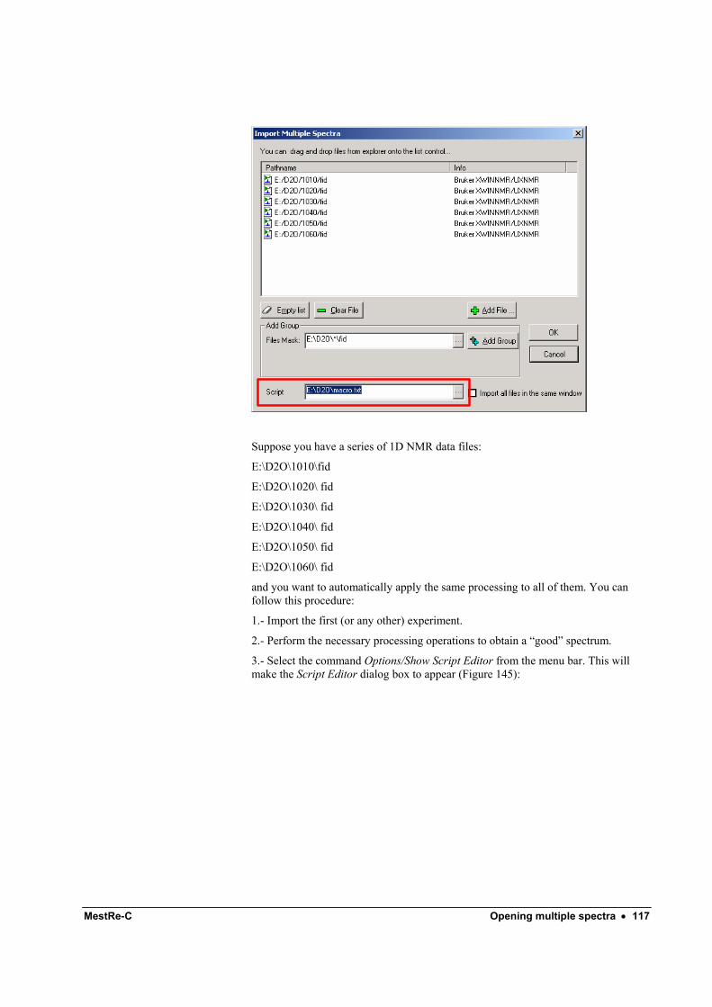
MestRe-C Opening multiple spectra • 117
Suppose you have a series of 1D NMR data files:
E:\D2O\1010\fid
E:\D2O\1020\ fid
E:\D2O\1030\ fid
E:\D2O\1040\ fid
E:\D2O\1050\ fid
E:\D2O\1060\ fid
and you want to automatically apply the same processing to all of them. You can follow this procedure:
1.- Import the first (or any other) experiment.
2.- Perform the necessary processing operations to obtain a “good” spectrum.
3.- Select the command Options/Show Script Editor from the menu bar. This will make the Script Editor dialog box to appear (Figure 145):
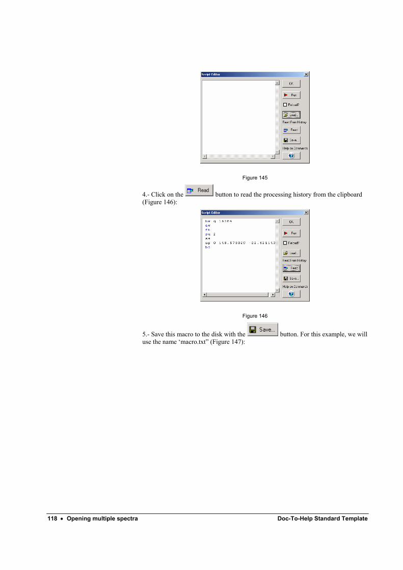
118 • Opening multiple spectra Doc-To-Help Standard Template
Figure 145
4.- Click on the button to read the processing history from the clipboard (Figure 146):
Figure 146
5.- Save this macro to the disk with the button. For this example, we will use the name ‘macro.txt” (Figure 147):
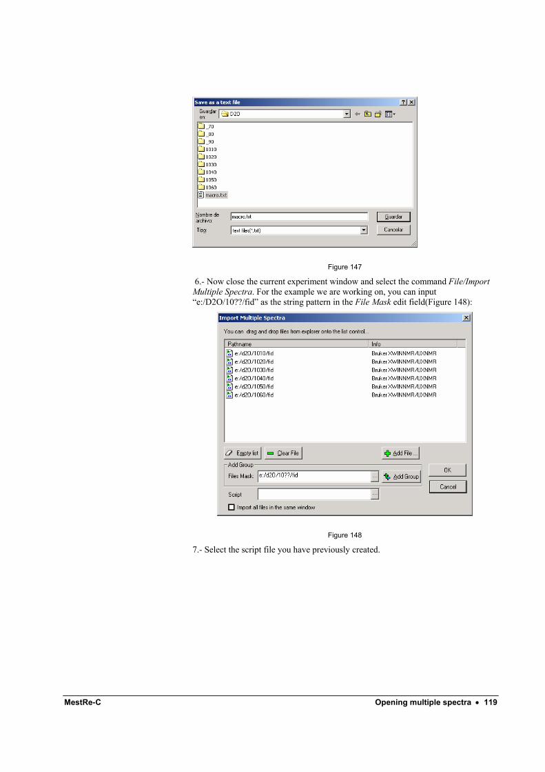
MestRe-C Opening multiple spectra • 119
Figure 147
6.- Now close the current experiment window and select the command File/Import Multiple Spectra. For the example we are working on, you can input “e:/D2O/10??/fid” as the string pattern in the File Mask edit field(Figure 148):
Figure 148
7.- Select the script file you have previously created.
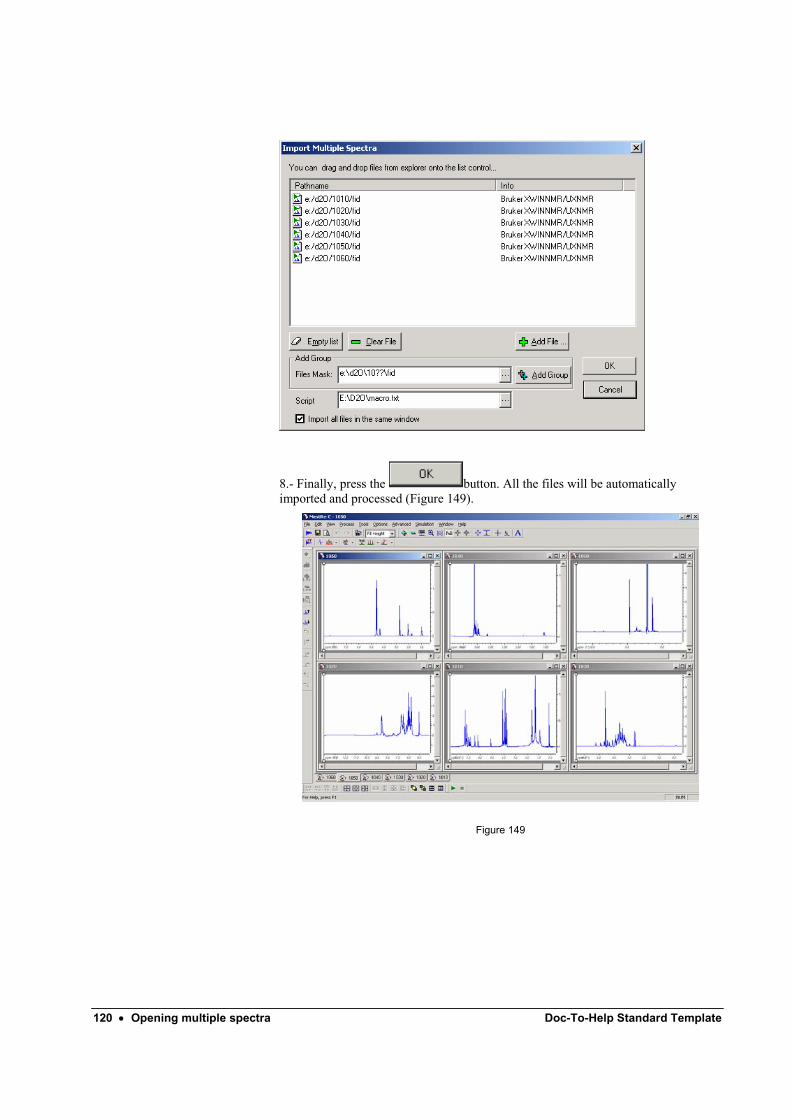
120 • Opening multiple spectra Doc-To-Help Standard Template
8.- Finally, press the button. All the files will be automatically imported and processed (Figure 149).
Figure 149
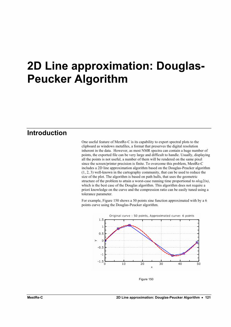
MestRe-C 2D Line approximation: Douglas-Peucker Algorithm • 121
2D Line approximation: Douglas-Peucker Algorithm
Introduction One useful feature of MestRe-C is its capability to export spectral plots to the clipboard as windows metafiles, a format that preserves the digital resolution inherent in the data. However, as most NMR spectra can contain a huge number of points, the exported file can be very large and difficult to handle. Usually, displaying all the points is not useful, a number of them will be rendered on the same pixel since the screen/printer precision is finite. To overcome this problem, MestRe-C includes a 2D line approximation algorithm based on the Douglas-Peucker algorithm (1, 2, 3) well-known in the cartography community, that can be used to reduce the size of the plot. The algorithm is based on path hulls, that uses the geometric structure of the problem to attain a worst-case running time proportional to nlog2(n), which is the best case of the Douglas algorithm. This algorithm does not require a priori knowledge on the curve and the compression ratio can be easily tuned using a tolerance parameter.
For example, Figure 150 shows a 50 points sine function approximated with by a 6 points curve using the Douglas-Peucker algorithm.
Figure 150
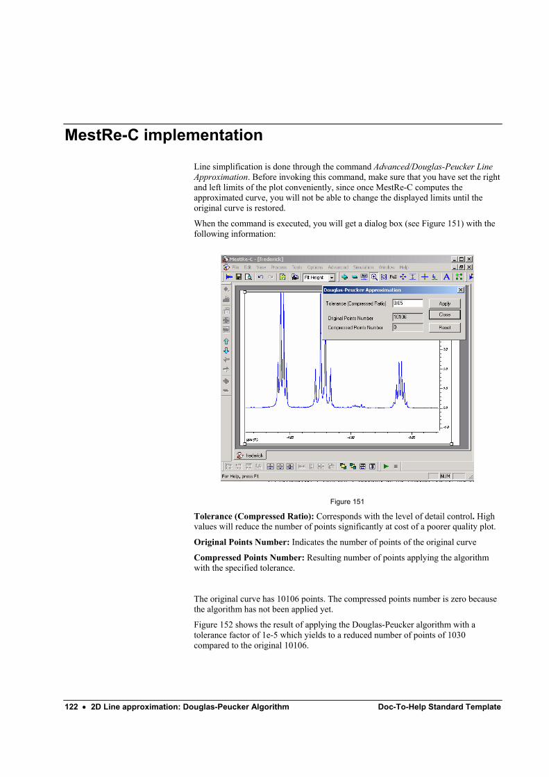
122 • 2D Line approximation: Douglas-Peucker Algorithm Doc-To-Help Standard Template
MestRe-C implementation
Line simplification is done through the command Advanced/Douglas-Peucker Line Approximation. Before invoking this command, make sure that you have set the right and left limits of the plot conveniently, since once MestRe-C computes the approximated curve, you will not be able to change the displayed limits until the original curve is restored.
When the command is executed, you will get a dialog box (see Figure 151) with the following information:
Figure 151
Tolerance (Compressed Ratio): Corresponds with the level of detail control. High values will reduce the number of points significantly at cost of a poorer quality plot.
Original Points Number: Indicates the number of points of the original curve
Compressed Points Number: Resulting number of points applying the algorithm with the specified tolerance.
The original curve has 10106 points. The compressed points number is zero because the algorithm has not been applied yet.
Figure 152 shows the result of applying the Douglas-Peucker algorithm with a tolerance factor of 1e-5 which yields to a reduced number of points of 1030 compared to the original 10106.
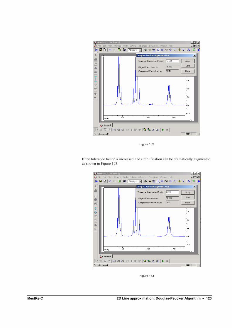
MestRe-C 2D Line approximation: Douglas-Peucker Algorithm • 123
Figure 152
If the tolerance factor is increased, the simplification can be dramatically augmented as shown in Figure 153:
Figure 153

124 • 2D Line approximation: Douglas-Peucker Algorithm Doc-To-Help Standard Template
(1) Douglas DH, Peucker TK. Can. Cartographer, 1973; 10(2): 112-122 (2) Hershberger J, Snoeyink J. Speeding up the Douglas-Peucker line simplification algorithm. In Proc. 5th Intl. Symp. Spatial Data Handling. IGU Commission on GIS, pages 134-143, 1992. (3) de Halleux J, An C++ implementation of Douglas-Peucker Line Approximation Algorithm. http://www.codeproject.com/useritems/dphull.asp
MestRe-C Running MestRe-C from the command line • 125
Running MestRe-C from the command line
Introduction MestRe-C can be run directly from the command line. This is useful if you want to include an instruction in a batch file to automatically open and process a certain experiment.
Loading an FID/spectrum To load an FID/spectrum, first pull up a command line prompt (go to the Start Menu, click Run and enter Command) and change to the system directory of your MestRe-C install (e.g. C:\MestRe-C). The syntax of the command to be issued is:
mestrec [FileName] [–m MacroFile] where [ ] are optional parameters.
[FileName] is the file name of the FID/spectrum to be opened. You have to include the complete file path to the document.
[–m MacroFile] is the file name of the macro file you want to apply to [FileName]
For example:
mestrec c:\sample.fid\fid.mrc –m c:\macro\mc.txt
loads the fid.mrc file from c:\sample.fid and applies the mc.txt macro located in c:\macro directory.
(Note the command is completely case insensitive)

126 • Running MestRe-C from the command line Doc-To-Help Standard Template
This option is not limited to MestRe-C’s own native files. You can include any file format supported by the program. For example, the following command will load a Varian’s FID:
mestrec c:\NMR\sample.fid\fid Note that you don’t need to specify the file format, MestRe-C will automatically do it for you.

MestRe-C Running MestRe-C from the command line • 127


Doc-To-Help Standard Template Running MestRe-C from the command line • 129


![bbb3 - tudehpartyiran.org · Æc h j= Äc ~ ¹c ~ ] Êc£¨v °c¨ y=] Çc{ ` c i Êc£ Åc¨ Êc £¨v c i [ c =¥cn c~ ccccccccccc i Çccccccccccc ccccccccccc£{ Çccccccccccc }](https://static.fdocument.org/doc/165x107/5e0dd5e8ca9d1b648e05c6ba/bbb3-c-h-j-c-c-cv-c-y-c-c-i-c-c-c-v.jpg)