
Measurement of CP violation in B0 /ψ decay L at … · Measurement of CP violation in B0 → J/ψ...
105
Measurement of CP violation in B 0 → J/ψ + K L decay at KEK B-factory Dissertation Graduate school of Tohoku University Mitsuhiro Yamaga February 2001
Transcript of Measurement of CP violation in B0 /ψ decay L at … · Measurement of CP violation in B0 → J/ψ...
Measurement of CP violationin B0 → J/ψ + KL decay
at KEK B-factory
Dissertation
Graduate school of Tohoku University
Mitsuhiro Yamaga
February 2001

Acknowledgment
I would like to thank everyone who helped me.First, I would like to thank my advisor, Prof. Yamaguchi, for his gentle support
and supervising my education of high energy physics.Since I have worked mainly at KEK, I have been under the care of the KEK
staffs. Especially, Prof. Kazuo Abe took great care of me over three years. I couldnot finish my work without his advice. I have no words to express my thanks tohim.
I also thank all the Belle collaborators for many suggestions.Finally I thank my wife, Atsuko Yamaga, for her support of my study as well as
my life .
Abstract
We have measured the CP asymmetry parameter sin 2φ1 in the B0 → J/ψ+KL
decay at KEK B-factory.For the detection of KL and muons, the KLM detector subsystem was con-
structed which was based on glass-electrode resistive plate chambers (RPC). Al-though this was the first time that the glass plates were used as the RPC electrode,performance of the system under the high luminosity runs was proved to be excellent.
Only the direction of hadron shower, which was created by KL, was measuredby a combination of the KLM detector and the electromagnetic calorimeter. TheB0 → J/ψ+KL signal was extracted from the center-of-mass momentum spectrumof the parent B0, which was determined by the measured J/ψ momentum and KL
angle and assuming the two body decay. This is the first direct measurement ofB0 → J/ψ +KL decay.
We observed 102 candidate events with an estimated background of 48 in the datasample of 6.2fb−1. Although statistics is still limited, we could successfully identifiedthe flavor ofB meson, and measured the difference of decay vertices of two B mesons.From the proper-time difference analysis, we obtained sin 2φ1 = −1.00 +0.89
−0.73.
Contents
1 Introduction 1
2 CP violation in B decays 32.1 Description with the Standard Model . . . . . . . . . . . . . . . . . . 32.2 The unitarity triangle . . . . . . . . . . . . . . . . . . . . . . . . . . . 52.3 CP violation in B0 meson system . . . . . . . . . . . . . . . . . . . . 6
2.3.1 B0 − B0 mixing . . . . . . . . . . . . . . . . . . . . . . . . . . 62.3.2 Interference between decay and mixing . . . . . . . . . . . . . 8
2.4 φ1 measurement . . . . . . . . . . . . . . . . . . . . . . . . . . . . . . 10
3 KEK B-factory 133.1 KEKB accelerator . . . . . . . . . . . . . . . . . . . . . . . . . . . . . 133.2 Belle detector . . . . . . . . . . . . . . . . . . . . . . . . . . . . . . . 14
3.2.1 Silicon Vertex Detector(SVD) . . . . . . . . . . . . . . . . . . 183.2.2 Central Drift Chamber (CDC) . . . . . . . . . . . . . . . . . . 183.2.3 Aerogel Cerenkov Counter (ACC) . . . . . . . . . . . . . . . . 193.2.4 Time of Flight counter (TOF/TSC) . . . . . . . . . . . . . . . 193.2.5 Electromagnetic Calorimeter(ECL) . . . . . . . . . . . . . . . 213.2.6 KL/µ detector (KLM) . . . . . . . . . . . . . . . . . . . . . . 223.2.7 Extreme Forward Calorimeter (EFC) . . . . . . . . . . . . . . 223.2.8 Trigger and data acquisition . . . . . . . . . . . . . . . . . . . 22
3.3 KEKB and Belle commissioning . . . . . . . . . . . . . . . . . . . . . 24
4 KLM detector 284.1 Introduction . . . . . . . . . . . . . . . . . . . . . . . . . . . . . . . . 284.2 Glass-electrode RPC . . . . . . . . . . . . . . . . . . . . . . . . . . . 304.3 Superlayer structure . . . . . . . . . . . . . . . . . . . . . . . . . . . 334.4 Gas system . . . . . . . . . . . . . . . . . . . . . . . . . . . . . . . . 334.5 HV system . . . . . . . . . . . . . . . . . . . . . . . . . . . . . . . . . 334.6 Readout system . . . . . . . . . . . . . . . . . . . . . . . . . . . . . . 354.7 Efficiency and resolution . . . . . . . . . . . . . . . . . . . . . . . . . 35
5 Software Tools 405.1 Overview . . . . . . . . . . . . . . . . . . . . . . . . . . . . . . . . . . 405.2 Reconstruction tools . . . . . . . . . . . . . . . . . . . . . . . . . . . 40
i

5.2.1 Charged particle tracking . . . . . . . . . . . . . . . . . . . . 40
5.2.2 Energy reconstruction . . . . . . . . . . . . . . . . . . . . . . 41
5.2.3 Particle Identification . . . . . . . . . . . . . . . . . . . . . . . 41
5.3 Monte Carlo simulation . . . . . . . . . . . . . . . . . . . . . . . . . . 46
5.3.1 Event generator . . . . . . . . . . . . . . . . . . . . . . . . . . 46
5.3.2 Full detector simulation . . . . . . . . . . . . . . . . . . . . . 46
5.3.3 Fast detector simulation . . . . . . . . . . . . . . . . . . . . . 46
6 KL detection 47
6.1 KL selection criteria . . . . . . . . . . . . . . . . . . . . . . . . . . . 47
6.2 Performance . . . . . . . . . . . . . . . . . . . . . . . . . . . . . . . . 49
6.2.1 Detection efficiency . . . . . . . . . . . . . . . . . . . . . . . . 49
6.2.2 Angular resolution . . . . . . . . . . . . . . . . . . . . . . . . 49
6.3 Verification of KL detection . . . . . . . . . . . . . . . . . . . . . . . 53
6.3.1 φ angular difference between KL and missing pt. . . . . . . . . 53
6.3.2 e+e− → γφ event . . . . . . . . . . . . . . . . . . . . . . . . . 54
6.4 KLM response in data and Monte Carlo . . . . . . . . . . . . . . . . 55
6.4.1 KLM cluster classification . . . . . . . . . . . . . . . . . . . . 55
6.4.2 KLM response to KL . . . . . . . . . . . . . . . . . . . . . . . 57
6.4.3 KLM response to π± and K± . . . . . . . . . . . . . . . . . . 58
6.4.4 Summary of KLM response to KL, π± and K± . . . . . . . . . 58
7 Reconstruction of B0 → J/ψ +KL decays 61
7.1 Data set and Monte Carlo events . . . . . . . . . . . . . . . . . . . . 61
7.2 Hadronic event selection . . . . . . . . . . . . . . . . . . . . . . . . . 61
7.3 J/ψ selection . . . . . . . . . . . . . . . . . . . . . . . . . . . . . . . 62
7.4 B0 → J/ψ +KL reconstruction . . . . . . . . . . . . . . . . . . . . . 63
7.5 Signal yield and background estimation . . . . . . . . . . . . . . . . . 70
8 Measurement of CP asymmetry 74
8.1 Flavor Tagging . . . . . . . . . . . . . . . . . . . . . . . . . . . . . . 74
8.2 Proper decay time difference . . . . . . . . . . . . . . . . . . . . . . . 77
8.3 Vertex reconstruction . . . . . . . . . . . . . . . . . . . . . . . . . . . 77
8.3.1 CP -side vertex . . . . . . . . . . . . . . . . . . . . . . . . . . 77
8.3.2 Tag-side vertex . . . . . . . . . . . . . . . . . . . . . . . . . . 78
8.4 Resolution function . . . . . . . . . . . . . . . . . . . . . . . . . . . . 78
8.4.1 Resolution function . . . . . . . . . . . . . . . . . . . . . . . . 78
8.4.2 Resolution function for background events . . . . . . . . . . . 80
8.5 CP fitting . . . . . . . . . . . . . . . . . . . . . . . . . . . . . . . . . 81
8.5.1 Fraction and CP of the background . . . . . . . . . . . . . . . 82
8.5.2 Result . . . . . . . . . . . . . . . . . . . . . . . . . . . . . . . 83
9 Conclusion 88
ii

A J/ψK∗(KLπ) reduction 90A.1 B− → J/ψK∗−(KLπ
−) . . . . . . . . . . . . . . . . . . . . . . . . . . 90A.2 B0 → J/ψK∗0(KLπ
0) . . . . . . . . . . . . . . . . . . . . . . . . . . . 90A.3 Summary . . . . . . . . . . . . . . . . . . . . . . . . . . . . . . . . . 93
Bibliography 94
iii
List of Figures
2.1 Unitarity triangle of KM matrix. . . . . . . . . . . . . . . . . . . . . 62.2 Box diagram for B0 − B0 mixing. . . . . . . . . . . . . . . . . . . . . 62.3 Diagram for B0 → J/ψKS. . . . . . . . . . . . . . . . . . . . . . . . . 112.4 Time dependent CP asymmetry measurement with B0 → J/ψKL. . . 12
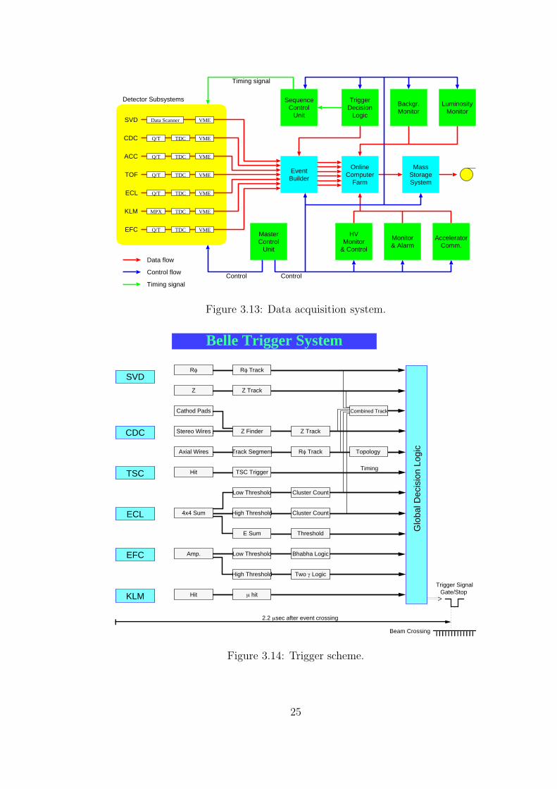
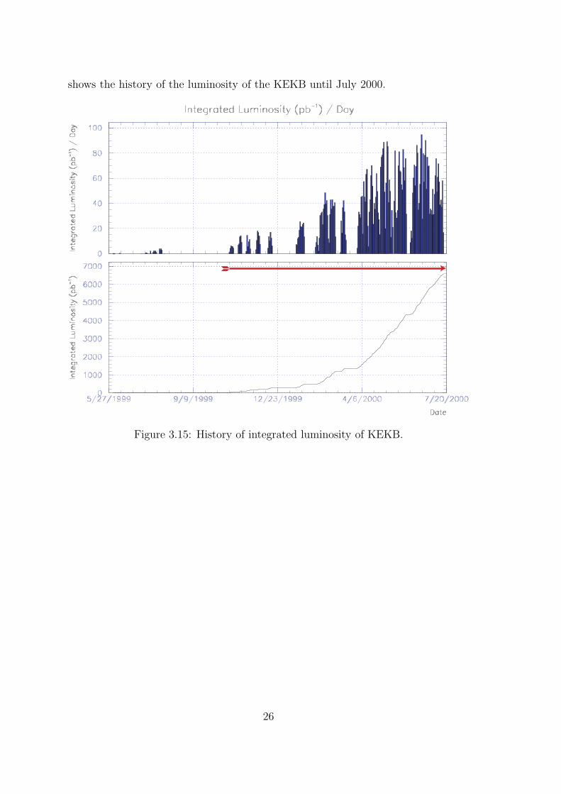
3.1 Required integrated luminosity to measure the CP asymmetry. . . . . 143.2 Configuration of KEKB accelerator. . . . . . . . . . . . . . . . . . . . 153.3 Belle detector. . . . . . . . . . . . . . . . . . . . . . . . . . . . . . . . 163.4 Side view of Belle detector. . . . . . . . . . . . . . . . . . . . . . . . . 173.5 Definition of Belle coordinate system. . . . . . . . . . . . . . . . . . . 173.6 Silicon Vertex Detector(SVD). . . . . . . . . . . . . . . . . . . . . . . 183.7 Central drift chamber (CDC). . . . . . . . . . . . . . . . . . . . . . . 193.8 Configuration of barrel ACC. . . . . . . . . . . . . . . . . . . . . . . 203.9 Configuration of endcap ACC. . . . . . . . . . . . . . . . . . . . . . . 203.10 Configuration of TOF/TSC. . . . . . . . . . . . . . . . . . . . . . . . 213.11 CsI calorimeter. . . . . . . . . . . . . . . . . . . . . . . . . . . . . . . 233.12 Extreme Forward Calorimeter. . . . . . . . . . . . . . . . . . . . . . . 243.13 Data acquisition system. . . . . . . . . . . . . . . . . . . . . . . . . . 253.14 Trigger scheme. . . . . . . . . . . . . . . . . . . . . . . . . . . . . . . 253.15 History of integrated luminosity of KEKB. . . . . . . . . . . . . . . . 26
4.1 Schematic view of barrel and endcap KLM. . . . . . . . . . . . . . . . 294.2 Typical signal of Glass-electrode RPC. . . . . . . . . . . . . . . . . . 304.3 Barrel RPC showing internal spacers. . . . . . . . . . . . . . . . . . . 314.4 Endcap RPC showing internal spacers. . . . . . . . . . . . . . . . . . 314.5 Cut-away view of an endcap RPC module. . . . . . . . . . . . . . . . 324.6 Superlayer structure. . . . . . . . . . . . . . . . . . . . . . . . . . . . 324.7 KLM gas distribution system. . . . . . . . . . . . . . . . . . . . . . . 344.8 KLM gas exhaust system. . . . . . . . . . . . . . . . . . . . . . . . . 344.9 Time multiplex scheme. . . . . . . . . . . . . . . . . . . . . . . . . . 354.10 Efficiency of endcap RPC module as a function of HV. . . . . . . . . 374.11 Efficiency map of RPC in endcap module. . . . . . . . . . . . . . . . 374.12 Spatial resolution of a superlayer. . . . . . . . . . . . . . . . . . . . . 384.13 Time resolution of KLM system. . . . . . . . . . . . . . . . . . . . . . 39
5.1 Flow of data analysis and Monte Carlo simulation. . . . . . . . . . . 41
iv
5.2 Efficiency and fake rate of electron identification. . . . . . . . . . . . 42
5.3 Efficiency and fake rate of muon identification. . . . . . . . . . . . . . 44
5.4 Momentum coverage of each component for K/π separation. . . . . . 45
5.5 Efficiency and fake rate of K by K/π separation routine. . . . . . . . 45
6.1 Schematic of KLM hit clustering and determination of its direction. . 48
6.2 Schematic of matching of charged track and KLM cluster. . . . . . . 48
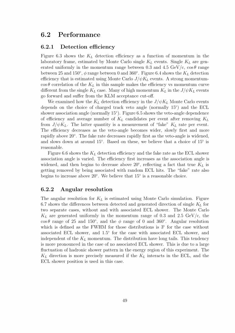
6.3 Momentum and cos θ dependence of KL detection efficiency deter-mined using single KL Monte Carlo events. . . . . . . . . . . . . . . . 50
6.4 Momentum and cos θ dependence of KL detection efficiency deter-mined using J/ψKL Monte Carlo events. . . . . . . . . . . . . . . . . 50
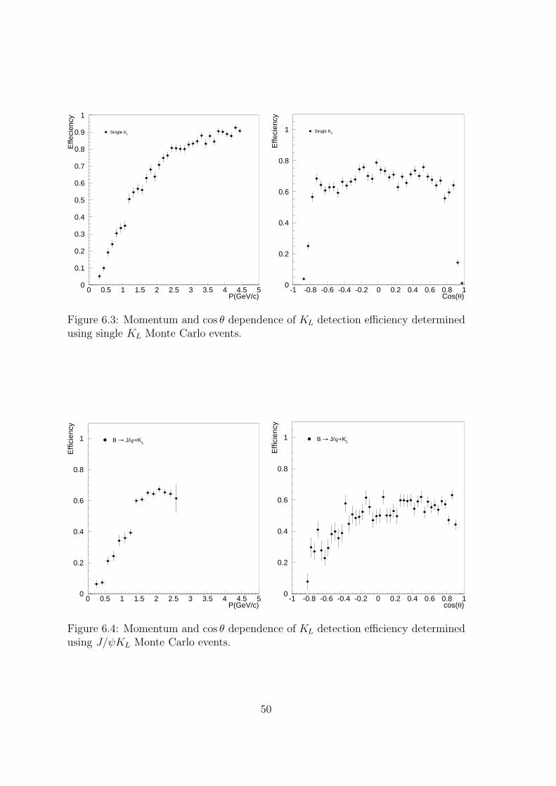
6.5 Charged track veto angle dependence of KL detection efficiency and“fake” KL fraction in the event. . . . . . . . . . . . . . . . . . . . . . 51
6.6 ECL association angle dependence of KL detection efficiency and“fake” rate. . . . . . . . . . . . . . . . . . . . . . . . . . . . . . . . . 51
6.7 Difference between detected and generated directions of KL. . . . . . 52
6.8 φ angular difference between theKL candidate direction and the miss-ing momentum vector direction. . . . . . . . . . . . . . . . . . . . . . 53
6.9 Feynman diagram of e+e− → γφ. . . . . . . . . . . . . . . . . . . . . 54
6.10 KL detection efficiency as a function of momentum measured bye+e− → γφ with data and Monte Carlo sample. . . . . . . . . . . . . 56
6.11 θ distribution of detected KL in data and Monte Carlo sample andits ratio. . . . . . . . . . . . . . . . . . . . . . . . . . . . . . . . . . . 57
6.12 θ and φ distribution of the fraction of making KLM clusters for pionsof momentum between 0.8 and 1.2 GeV/c. . . . . . . . . . . . . . . . 59
6.13 The fraction of pions making KLM clusters, and the ratio of data tothe Monte Carlo. . . . . . . . . . . . . . . . . . . . . . . . . . . . . . 59
6.14 θ and φ distribution of the fraction of making KLM clusters for kaonsof momentum between 0.8 and 1.2 GeV/c. . . . . . . . . . . . . . . . 60
6.15 The fraction of kaons making KLM clusters, and the ratio of data tothe Monte Carlo. . . . . . . . . . . . . . . . . . . . . . . . . . . . . . 60
7.1 Dilepton mass distribution. . . . . . . . . . . . . . . . . . . . . . . . . 63
7.2 Momentum spectrum of J/ψ candidates. . . . . . . . . . . . . . . . . 64
7.3 Calculated KL momentums. . . . . . . . . . . . . . . . . . . . . . . . 66
7.4 Scatter plots of p∗J/ψ versus p∗B. . . . . . . . . . . . . . . . . . . . . . 67
7.5 p∗B distribution of the data after p∗J/ψ cut. . . . . . . . . . . . . . . . . 68
7.6 A typical example of J/ψKL candidate event projected on X−Y plane. 69
7.7 p∗B distribution when all KL in an event are rotated by 180 in φbefore reconstruction. . . . . . . . . . . . . . . . . . . . . . . . . . . . 71
7.8 p∗B distribution of Monte Carlo and fitted curves. . . . . . . . . . . . 72
7.9 p∗B distribution with the fit result. . . . . . . . . . . . . . . . . . . . . 73
8.1 Illustration for the flavor tagging method. . . . . . . . . . . . . . . . 75
8.2 Illustration for vertex reconstruction of two B decay vertices. . . . . . 78
v

8.3 (a) σtrackz distribution, (b) δz distribution and (c) δr distribution inthe data. . . . . . . . . . . . . . . . . . . . . . . . . . . . . . . . . . . 79
8.4 The average shape of the event-by-event resolution function obtainedby summing over 440 B− → D0π− events. . . . . . . . . . . . . . . . 80
8.5 The p∗B dependence of the fraction of signal, background with CPasymmetry, and background without CP asymmetry. . . . . . . . . . 82
8.6 The ∆t distribution in the “blind analysis” for the events in the signalp∗B region. . . . . . . . . . . . . . . . . . . . . . . . . . . . . . . . . . 84
8.7 The ∆t distribution after tagging the flavor of B0 meson. . . . . . . . 868.8 The ∆t distribution and the CP fit result for the events in the signal
p∗B region. . . . . . . . . . . . . . . . . . . . . . . . . . . . . . . . . . 87
A.1 Monte Carlo results of p∗B vs mKπ for J/ψKL and for J/ψK∗−(KLπ−). 91
A.2 Monte Carlo results of p∗B vs mKπ for J/ψKL and for J/ψK∗0(KLπ0). 92
vi

List of Tables
3.1 Parameters of KEKB. . . . . . . . . . . . . . . . . . . . . . . . . . . 27
6.1 Number of KLM clusters per event and their classification. . . . . . . 576.2 Fractions of KL clusters which use KLM only and which is associated
with ECL. . . . . . . . . . . . . . . . . . . . . . . . . . . . . . . . . . 57
7.1 Result of fit to the p∗B distribution. . . . . . . . . . . . . . . . . . . . 70
8.1 Summary of the tagging efficiencies (ε), wrong tag fractions (ω) andeffective tagging efficiencies (εeff ). . . . . . . . . . . . . . . . . . . . . 77
8.2 Monte Carlo estimation of measurement accuracy for the CP -side z,tag-side z and ∆z. . . . . . . . . . . . . . . . . . . . . . . . . . . . . 81
8.3 Background in the B0 → J/ψ + KL candidate events and their CPasymmetry. . . . . . . . . . . . . . . . . . . . . . . . . . . . . . . . . 83
A.1 Reduction of signal and background candidates in the J/ψK∗−(KLπ−). 91
A.2 Use of vertex information in the J/ψK∗−(KLπ−) analysis starting
from the event sample that passed the p∗B(3-body)-mKπ cut. . . . . . 91A.3 Reduction of signal and background candidates in the J/ψK∗0(KLπ
0). 92
vii

Chapter 1
Introduction
It is well known that the parity transformation P is violated in the weak interaction.This can be observed in the charged weak interaction where P is maximally parity-violating, that the charged vector boson W± couples only to left-handed fermionsand right-handed antifermion. However, the Lagrangian for the weak interactionis invariant under the combined operations of P and charge conjugation C if thecouplings have no physically significant phases.
The first observation of CP violation in the neutral kaon system in 1964 [1]suggested the existence of non-trivial phases in some cases of the weak couplings,and an enormous amount of theoretical work has been made to understand suchmechanism. In a remarkable paper published in 1973, Kobayashi and Maskawanoted that CP violation could be accommodated in the Standard Model only ifthere were at least six quark flavors, twice the number of quark flavors known atthat time [2]. The subsequent discovery of the c quark at SLAC [3] and BNL [4],and the b quark at Fermilab [5], and the t quark at CDF , has substantiated the six-quark Kobayashi-Maskawa (KM) hypothesis, and the KM model for CP violation isnow considered to be an essential part of the Standard Model.
In 1980, Sanda and Carter pointed out that the KM model contained the pos-sibility of large CP violating asymmetries in certain decay modes of the B mesons[6]. The subsequent observation of a long b quark lifetime [7] and a large amount ofmixing in the neutral B meson system indicated that it would be feasible to carryout decisive tests of the KM model by studying B meson decays.
The observation of a CP violating asymmetry in B meson decays would bean important milestone; the first successful demonstration of a CP violating effectoutside of the K0 meson system; and would be a dramatic confirmation of the KMmodel. The importance of the research of CP violation in B decays is reflected inthe number of laboratories. The BaBar [8] experiment at SLAC and CDF [9] arethe competitive experiment with Belle. Other projects addressing this physics isalso planned for LHC [10]. The goal of the Belle experiment at the first stage is toestablish the CP violation in B decays.
In this thesis, we present a measurement of the CP asymmetry angle sin 2φ1
in the B0 → J/ψ + KL decay using data collected by the Belle detector at KEKB-factory.
1

The outline of this thesis is as follows.
• First, physics formalism for CP violation is given in Chapter 2.
• An overview of experimental apparatus, KEK B-factory system which consistsof KEKB accelerator and Belle detector is described in Chapter 3.
• Detailed description of the KLM detector system is given in Chapter 4.
• Software tools for data analysis and Monte Carlo simulation are described inChapter 5.
• KL reconstruction method and performance are described in Chapter 6.
• Reconstruction procedure of B0 → J/ψ+KL decay is described in Chapter 7.
• Extraction of CP asymmetry parameter sin 2φ1 is described in Chapter 8.
• Finally, conclusion is given in Chapter 9.
2
Chapter 2
CP violation in B decays
In this chapter we describe the basic theory of CP violation in B decays and themeasurement of the angles of unitarity triangle.
2.1 Description with the Standard Model
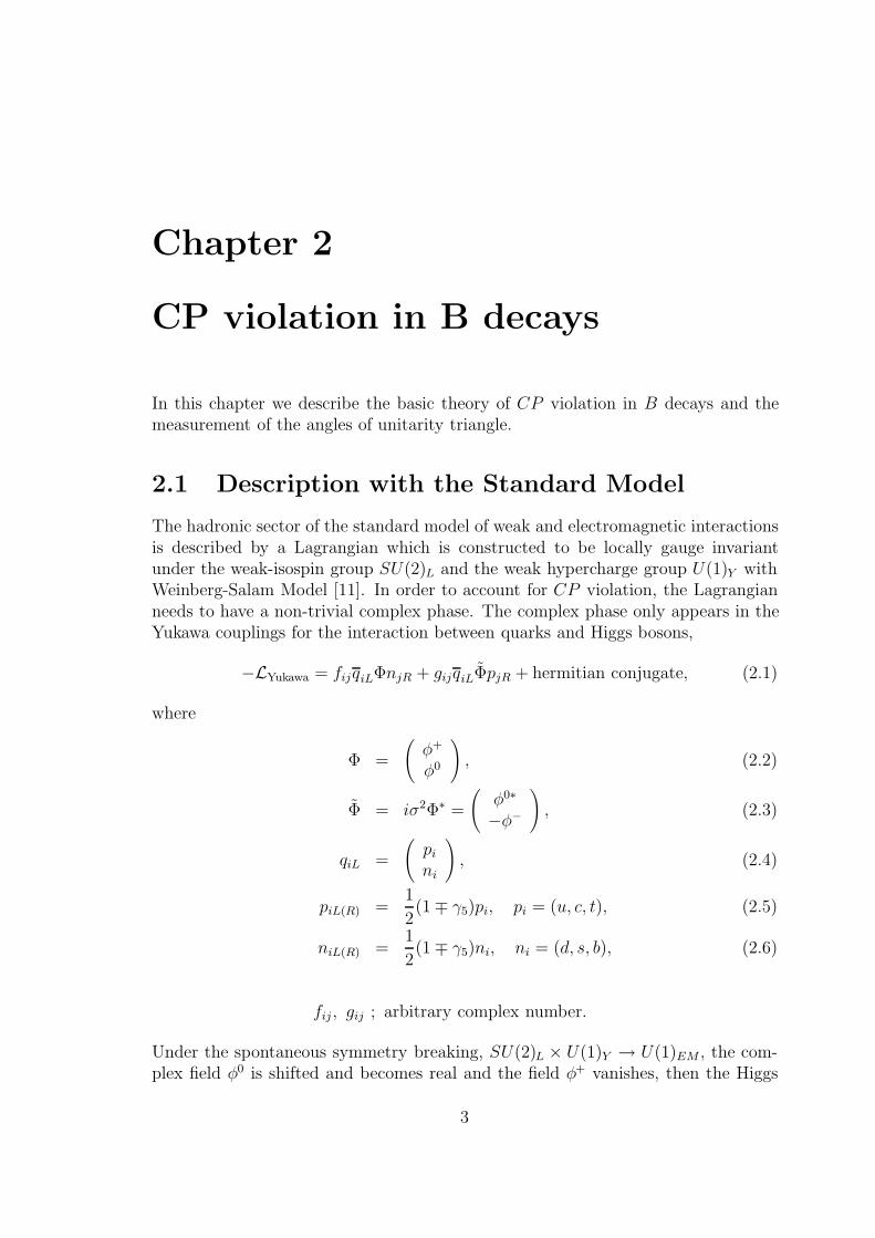
The hadronic sector of the standard model of weak and electromagnetic interactionsis described by a Lagrangian which is constructed to be locally gauge invariantunder the weak-isospin group SU(2)L and the weak hypercharge group U(1)Y withWeinberg-Salam Model [11]. In order to account for CP violation, the Lagrangianneeds to have a non-trivial complex phase. The complex phase only appears in theYukawa couplings for the interaction between quarks and Higgs bosons,
−LYukawa = fijqiLΦnjR + gijqiLΦpjR + hermitian conjugate, (2.1)
where
Φ =
(φ+
φ0
), (2.2)
Φ = iσ2Φ∗ =
(φ0∗
−φ−
), (2.3)
qiL =
(pini
), (2.4)
piL(R) =1
2(1 ∓ γ5)pi, pi = (u, c, t), (2.5)
niL(R) =1
2(1 ∓ γ5)ni, ni = (d, s, b), (2.6)
fij , gij ; arbitrary complex number.
Under the spontaneous symmetry breaking, SU(2)L × U(1)Y → U(1)EM , the com-plex field φ0 is shifted and becomes real and the field φ+ vanishes, then the Higgs
3
has a vacuum expectation value, 〈φ〉0,
〈φ〉0 =1√2
(0v
). (2.7)
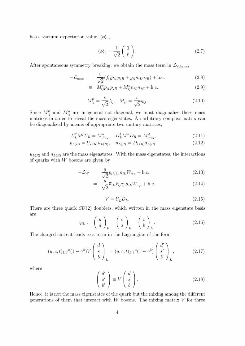
After spontaneous symmetry breaking, we obtain the mass term in LYukawa,
−Lmass =v√2(fijpiLpjR + gijniLnjR) + h.c. (2.8)
≡ MpijpiLpjR +Mn
ijniLnjR + h.c., (2.9)
Mpij =
v√2fij, Mn
ij =v√2gij. (2.10)
Since Mpij and Mn
ij are in general not diagonal, we must diagonalize these massmatrices in order to reveal the mass eigenstates. An arbitrary complex matrix canbe diagonalized by means of appropriate two unitary matrices;
U †LM
pUR = Mudiag, D†
LMnDR = Md
diag, (2.11)
pL(R) = UL(R)uL(R), nL(R) = DL(R)dL(R). (2.12)
uL(R) and nL(R) are the mass eigenstates. With the mass eigenstates, the interactionsof quarks with W bosons are given by
−LW =g√2piLγµniLW+µ + h.c. (2.13)
=g√2uiLVijγµdiLW+µ + h.c., (2.14)
V = U †LDL. (2.15)
There are three quark SU(2) doublets, which written in the mass eigenstate basisare
qiL :
(ud
)L
(cs
)L
(tb
)L
. (2.16)
The charged current leads to a term in the Lagrangian of the form
(u, c, t)Lγµ(1 − γ5)V
⎛⎜⎝ dsb
⎞⎟⎠L
= (u, c, t)Lγµ(1 − γ5)
⎛⎜⎝ d′
s′
b′
⎞⎟⎠L
, (2.17)
where ⎛⎜⎝d′
s′
b′
⎞⎟⎠ ≡ V
⎛⎜⎝dsb
⎞⎟⎠ . (2.18)
Hence, it is not the mass eigenstates of the quark but the mixing among the differentgenerations of them that interact with W bosons. The mixing matrix V for three
4
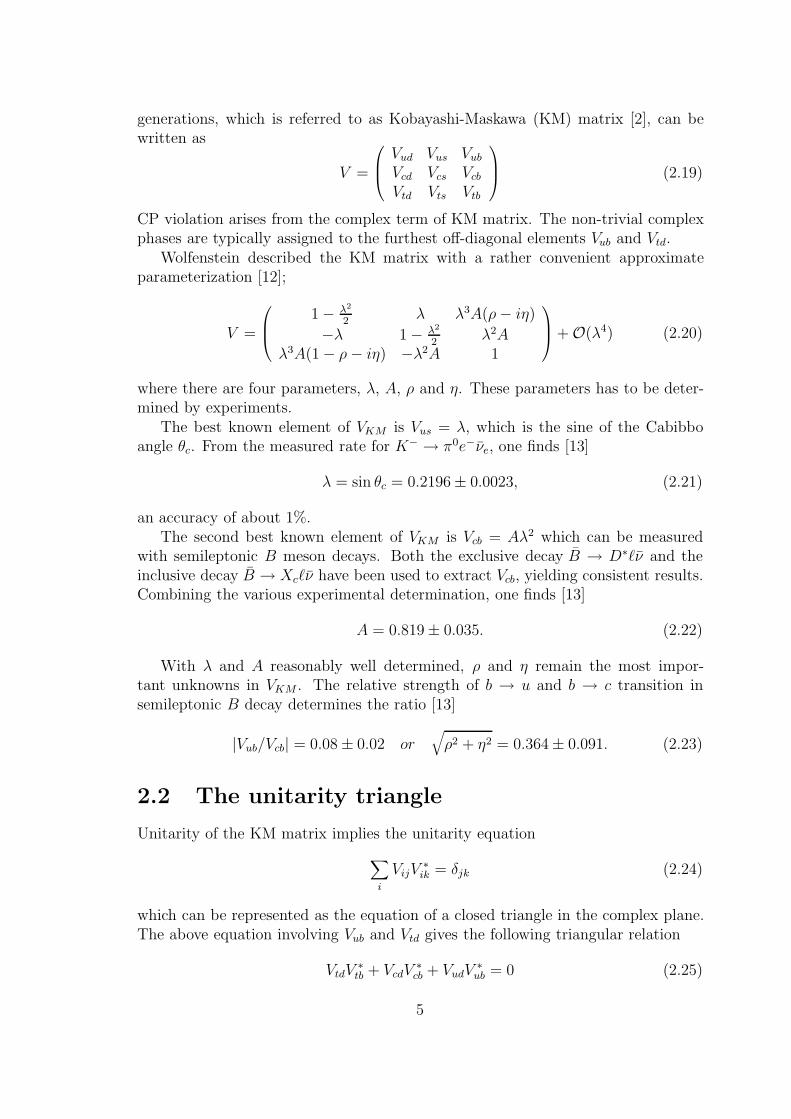
generations, which is referred to as Kobayashi-Maskawa (KM) matrix [2], can bewritten as
V =
⎛⎜⎝ Vud Vus VubVcd Vcs VcbVtd Vts Vtb
⎞⎟⎠ (2.19)
CP violation arises from the complex term of KM matrix. The non-trivial complexphases are typically assigned to the furthest off-diagonal elements Vub and Vtd.
Wolfenstein described the KM matrix with a rather convenient approximateparameterization [12];
V =
⎛⎜⎝
1 − λ2
2λ λ3A(ρ− iη)
−λ 1 − λ2
2λ2A
λ3A(1 − ρ− iη) −λ2A 1
⎞⎟⎠+ O(λ4) (2.20)
where there are four parameters, λ, A, ρ and η. These parameters has to be deter-mined by experiments.
The best known element of VKM is Vus = λ, which is the sine of the Cabibboangle θc. From the measured rate for K− → π0e−νe, one finds [13]
λ = sin θc = 0.2196 ± 0.0023, (2.21)
an accuracy of about 1%.The second best known element of VKM is Vcb = Aλ2 which can be measured
with semileptonic B meson decays. Both the exclusive decay B → D∗ν and theinclusive decay B → Xcν have been used to extract Vcb, yielding consistent results.Combining the various experimental determination, one finds [13]
A = 0.819 ± 0.035. (2.22)
With λ and A reasonably well determined, ρ and η remain the most impor-tant unknowns in VKM . The relative strength of b → u and b → c transition insemileptonic B decay determines the ratio [13]
|Vub/Vcb| = 0.08 ± 0.02 or√ρ2 + η2 = 0.364 ± 0.091. (2.23)
2.2 The unitarity triangle
Unitarity of the KM matrix implies the unitarity equation
∑i
VijV∗ik = δjk (2.24)
which can be represented as the equation of a closed triangle in the complex plane.The above equation involving Vub and Vtd gives the following triangular relation
VtdV∗tb + VcdV
∗cb + VudV
∗ub = 0 (2.25)
5

2φ
cd VV cb*
udVV ub* td VV tb*
3φ 1φ
Figure 2.1: Unitarity triangle of KM matrix.
which is the most useful one from the phenomenological point of view since it con-tains the most poorly-known elements in the KM matrix. This triangle has theshape shown in Figure 2.1. CP is violated when the area of the triangle does notvanish, i.e. when all the angles are different from zero. The three internal anglesare defined as
φ1 ≡ arg
(VcdV
∗cb
VtdV∗tb
), φ2 ≡ arg
(VudV
∗ub
VtdV∗tb
), φ3 ≡ arg
(VcdV
∗cb
VudV∗ub
)(2.26)
2.3 CP violation in B0 meson system
2.3.1 B0 − B0 mixing
The flavor state B0 and B0 mix through the weak interaction. Figure 2.2 shows thebox diagram for B0 − B0 mixing in the standard model.
B0 B0 B0 B0
d
b
b
dW
W
b
bd
du,c,t
u,c,t
u,c,t
u,c,tW W
Figure 2.2: Box diagram for B0 − B0 mixing.
The B meson state can be expressed as
|ΨB(t)〉 = a(t)|B0〉 + b(t)|B0〉, (2.27)
6
or
ΨB(t) =(a(t)b(t)
), (2.28)
which obeys the time-dependent Schrodinger equation
i∂
∂t|ΨB(t)〉 = H|ΨB(t)〉 = E|ΨB(t)〉. (2.29)
a and b are normalized as |a(t)|2 + |b(t)|2 = 1 . The Hamiltonian H is a 2×2 matrixwhich is expressed as
H =(H11 H12
H21 H22
)=
( 〈B0|H|B0〉 〈B0|H|B0〉〈B0|H|B0〉 〈B0|H|B0〉
)(2.30)
Considering that the wave function of decay particle is generally written as Ψ(t) =
Ψ(0)e−i(m− i2Γ)t, H is written as
H = M − i
2Γ (2.31)
where M (mass matrix) and Γ (decay matrix) are Hermitian 2 × 2 matrices,
M =(M11 M12
M21 M22
), Γ =
(Γ11 Γ12
Γ21 Γ22
), (2.32)
Since M and Γ are Hermitian,
M21 = M∗12, Γ21 = Γ∗
12. (2.33)
According to the CPT invariance, we obtain the relation
M11 = M22, Γ11 = Γ22. (2.34)
Here we obtain the expression
H =
( 〈B0|H|B0〉 〈B0|H|B0〉〈B0|H|B0〉 〈B0|H|B0〉
)=(M0 − i
2Γ0 M12 − i
2Γ12
M∗12 − i
2Γ∗
12 M0 − i2Γ0
)(2.35)
where M11 = M22 = M0、Γ11 = Γ22 = Γ0. The eigenstate of this Hamiltonian is themass-eigenstate of real particle. Let us call the two state as “heavy” (= BH) and“light” (= BL). We obtain the eigenstate (|BH〉、|BL〉) and eigenvalue (λH、λL)for each state as follows :
|BH〉 =1√
|p|2 + |q|2p|B0〉 − q|B0〉,
|BL〉 =1√
|p|2 + |q|2p|B0〉 + q|B0〉,
λH = M11 − i
2Γ11 − pq ≡ mH − i
2ΓH ,
λL = M11 − i
2Γ11 + pq ≡ mL − i
2ΓL, (2.36)
7
where
p = (M12 − i
2Γ12)
1/2,
q = (M∗12 −
i
2Γ∗
12)1/2. (2.37)
Define the mass difference ∆mB ≡ mH − mL and the width difference ∆ΓB ≡ΓH − ΓL. The solution for mixing parameter is
q
p=
√√√√M∗12 − i
2Γ∗
12
M12 − i2Γ12
= −2(M∗
12 − i2Γ∗
12
)∆mB − i
2∆ΓB
(2.38)
An alternative common notation is to define ε such that
p =1 + ε√
2 (1 + |ε|2), q =
1 − ε√2 (1 + |ε|2)
,q
p=
1 − ε
1 + ε. (2.39)
The condition ∣∣∣∣∣qp∣∣∣∣∣ = 1 (2.40)
implies indirect CP violation, which results from the fact that the mass eigenstatesare different from the CP eigenstates.
Although the ∆ΓB has not been measured directly, since the decay channelscommon to B0 and B0, which are responsible for the difference of ∆ΓB, are knownto have the branching fractions of order 10−3 or less, it should follow that ∆ΓB/ΓB <10−2. On the other hand, the observed B0−B0 mixing rate implies xd ≡ ∆mB/ΓB =0.74 ± 0.04 [14], i.e.
|∆ΓB| ∆mB. (2.41)
Thus there is a negligible lifetime difference between the mass eigenstates. It followsthat |Γ12| |M12|, and to first order in Γ12/M12 we obtain from (2.38)
q
p − M∗
12
|M12|(1 − 1
2Im
Γ12
M12
). (2.42)
Hence
1 −∣∣∣∣∣qp∣∣∣∣∣ 2Re ε ∼ O(10−2). (2.43)
CP violation in B0 − B0 mixing is a small effect as that in the kaon system.
2.3.2 Interference between decay and mixing
With mH,L = mB± 12∆mB and ΓH,L ΓB, we obtain the time evolution of the state
as
|BH(t)〉 = |BH〉e−i(mH− i2ΓB)t,
|BL(t)〉 = |BL〉e−i(mL− i2ΓB)t. (2.44)
8
From this equation we obtain the time evolution of |B0〉 and |B0〉.
|B0(t)〉 = g+(t)|B0〉 +q
pg−(t)|B0〉,
|B0(t)〉 =
p
qg−(t)|B0〉 + g+(t)|B0〉, (2.45)
where
g+(t) = e−i(mB− i2ΓB)t cos(
1
2∆mBt),
g−(t) = ie−i(mB− i2ΓB)t sin(
1
2∆mBt). (2.46)
Consider that initially pure B0 or B0 decays into the CP eigenstate fCP . Dueto B0 − B0 mixing, there exist two decay channels,
B0 → fCP , B0 → B0 → fCP (2.47)
Define the decay amplitudes as
A ≡ 〈fCP |B0〉, A ≡ 〈fCP |B0〉. (2.48)
For convenience we use
λ ≡ q
p
AA . (2.49)
It can be shown that λ is independent of phase conventions and thus physicallymeaningful. In other words, the convention dependence of q/p cancels against thatof A/A.
The time-dependent decay amplitude from Equation (2.45) is expressed as
〈fCP |B0(t)〉 = A[g+(t) + λg−(t)], (2.50)
〈fCP |B0(t)〉 = A
(p
q
)[g−(t) + λg+(t)]. (2.51)
Thus we obtain the time-dependent decay width as
Γ(B0(t) → fCP ) = |A|2e−ΓBt[1 + |λ|2
2+
1 − |λ|22
cos(∆mBt) − Imλ sin(∆mBt)],
Γ(B0(t) → fCP ) = |A|2e−ΓBt[
1 + |λ|22
− 1 − |λ|22
cos(∆mBt) + Imλ sin(∆mBt)].
(2.52)
Now we define the time-dependent CP asymmetry,
AfCP(t) ≡ Γ(B0(t) → fCP ) − Γ(B0(t) → fCP )
Γ(B0(t) → fCP ) + Γ(B0(t) → fCP ). (2.53)
Using Equation (2.52) it is expressed as
AfCP(t) =
(1 − |λ|2) cos(∆mBt) − 2Imλ sin(∆mBt)
1 + |λ|2 , (2.54)
9
In case of neutral B meson, |Γ12| ‖M12|, so q/p is approximately
q
p=
√√√√M∗12 − i
2Γ∗
12
M12 − i2Γ12
≈√M∗
12
M12, (2.55)
and hence |q/p| = 1. Also note that if a single combination of quark-mixing-matrixelements contributes to B0 → fCP and B0 → fCP , |A/A| = 1. Therefore
|λ| =
∣∣∣∣∣qp∣∣∣∣∣∣∣∣∣∣AA∣∣∣∣∣ = 1. (2.56)
Thus Equation (2.54) becomes
AfCP(t) −Imλ sin(∆mBt) (2.57)
This method using such decays is very useful and shows large CP violation in theStandard Model prediction. The quantity Imλ which can be extracted from AfCP
istheoretically very interesting since it can be directly related to KM matrix elementsin the Standard Model.
2.4 φ1 measurement
• B0 → J/ψKS
One of the cleanest example that we can measure the unitarity angle is the B0 →J/ψKS via b → ccs quark transition. B0 → J/ψKS → +−π+π− is the mostpromising mode since the branching ratio for this mode has been measured andthe signals are very clean with no appreciable background. Figure 2.3 shows theFeynman diagram for this decay.
In the B meson system, up to corrections of order 10−2, we have
(q
p
)√M∗
12
M12=V ∗tbVtdVtbV ∗
td
= e−2iφ1 . (2.58)
This combination of KM parameters can be read off directly from the vertices ofthe box diagram in Figure 2.2, which in the Standard Model are responsible for thenon-diagonal element M∗
12 of the mass matrix. As shown in Figure 2.3, the weakphase in the tree diagram is represented by V ∗
cbVcs. With CP (J/ψKS) = −1, onefinds
λJ/ψKS= −
(q
p
)B
·(q
p
)K
· AA =V ∗tbVtdVtbV ∗
td
· VcsVcdV ∗csVcd
· VcbV∗cs
V ∗cbVcs
= −e−2iφ1 , (2.59)
where the first term comes from B0 − B0 mixing, the second from the ratio Af/Af
and the third from K0 − K0 mixing. Therefore we obtain
ImλJ/ψKS sin 2φ1. (2.60)
10
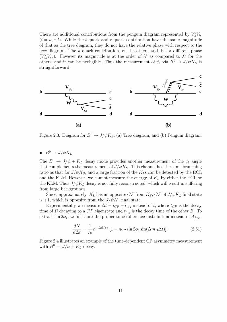
There are additional contributions from the penguin diagram represented by V ∗ibVis
(i = u, c, t). While the t quark and c quark contribution have the same magnitudeof that as the tree diagram, they do not have the relative phase with respect to thetree diagram. The u quark contribution, on the other hand, has a different phase(V ∗
ubVus). However its magnitude is at the order of λ4 as compared to λ2 for theothers, and it can be negligible. Thus the measurement of φ1 via B0 → J/ψKS isstraightforward.
b– Vcb c
–
dd
WVcs
c
s–
(a)
b– Vib Vis s
–
dd
c
c–
W
(b)
Figure 2.3: Diagram for B0 → J/ψKS, (a) Tree diagram, and (b) Penguin diagram.
• B0 → J/ψKL
The B0 → J/ψ + KL decay mode provides another measurement of the φ1 anglethat complements the measurement of J/ψKS. This channel has the same branchingratio as that for J/ψKS, and a large fraction of the KLs can be detected by the ECLand the KLM. However, we cannot measure the energy of KL by either the ECL orthe KLM. Thus J/ψKL decay is not fully reconstructed, which will result in sufferingfrom large backgrounds.
Since, approximately, KL has an opposite CP from KS, CP of J/ψKL final stateis +1, which is opposite from the J/ψKS final state.
Experimentally we measure ∆t = tCP − ttag instead of t, where tCP is the decaytime of B decaying to a CP eigenstate and ttag is the decay time of the other B. Toextract sin 2φ1, we measure the proper time difference distribution instead of AfCP
,
dN
d∆t=
1
τBe−|∆t|/τB [1 − ηCP sin 2φ1 sin(∆mB∆t)] . (2.61)
Figure 2.4 illustrates an example of the time-dependent CP asymmetry measurementwith B0 → J/ψ +KL decay.
11

e (8.0GeV) e (3.5GeV)
CP decay
Tagged decay
B
_B
0
0
∆z~βγc∆t
KL
e, µ
e, µ
- +
Figure 2.4: Time dependent CP asymmetry measurement with B0 → J/ψKL.
12
Chapter 3
KEK B-factory
KEK B-factory consists of an asymmetric high luminosity e+e− collider and detectorsystem built at KEK (High Energy Accelerator and Research Organization, Japan).KEKB accelerator is designed to produce a large number of B mesons. The Belledetector is optimized to measure the particles from B meson decays effectively.
In this chapter we describe the experimental apparatus of KEK B-factory. KEKBaccelerator specification, Belle detector system with sub detector components anddata acquisition system are described.
3.1 KEKB accelerator
KEKB accelerator is an e+e− collider with asymmetric beam energies. The centerof mass energy is set to 10.58 GeV which is on the Υ(4S) resonance state. SinceΥ(4S) decays only into B meson pairs, we can generate B meson pairs efficiently.In the Υ(4S) rest frame, the average momentum of B meson in the Υ(4S) decay isabout 340 MeV/c, so the average decay length is approximately 30 µm. This lengthis too short to measure the difference of the vertex of two B mesons by presentvertex detector. So Υ(4S) is Lorentz boosted so that the flight length of B mesonsare long enough to be measured by the vertex detector. The asymmetry of beamenergy is expressed as
βγ =E− − E+√
s
where βγ is the Lorentz boost parameter,√s is the center of mass energy, and E−
and E+ are the energy of electron and positron, respectively. There are two factorsto optimize this asymmetry. One is the flight length of the B mesons, and the otheris the detector acceptance. Figure 3.1 shows the required integrated luminosity asa function of βγ to measure the CP asymmetry parameter, sin 2φ1, with 3σ. Itdoes not change so significantly within the range of 0.4 to 0.8. Thus the asymmetrywas determined to be βγ = 0.425, and the energy of electron and positron is set toE− = 8.0 GeV and E+ = 3.5 GeV. The average decay length is approximately 200µm in this case.
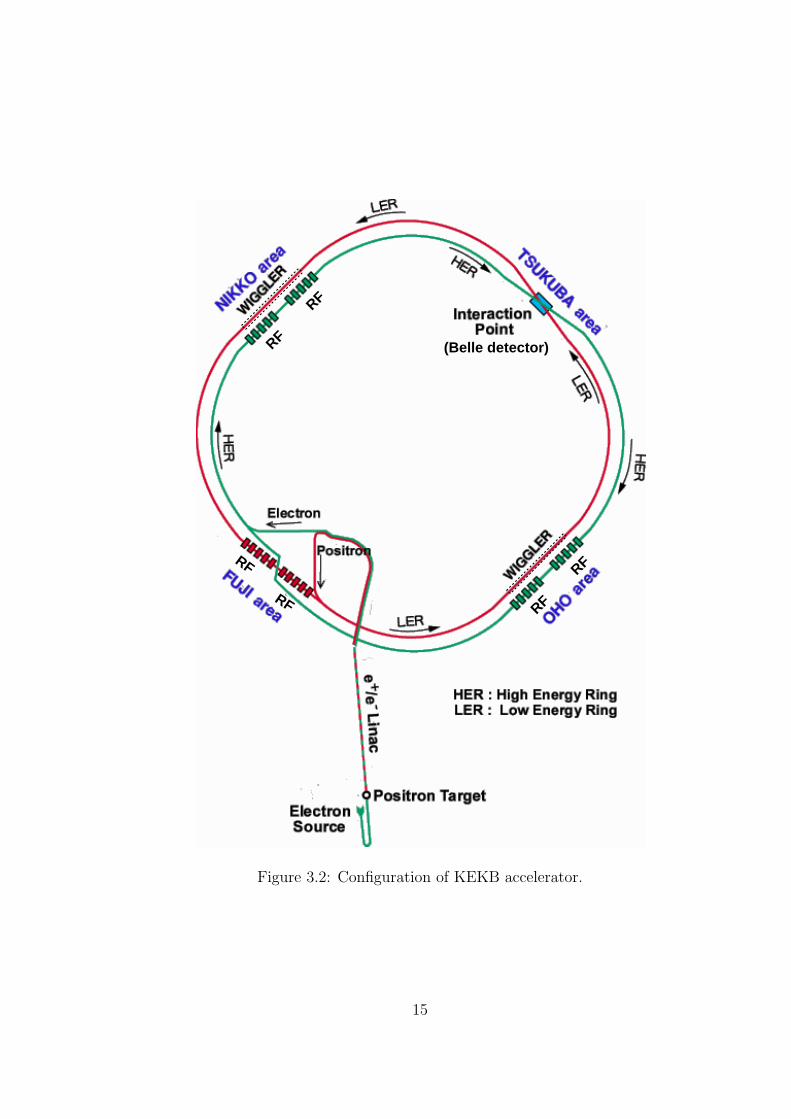
Figure 3.2 shows the overview of KEKB [15]. The electron ring (HER:High
13
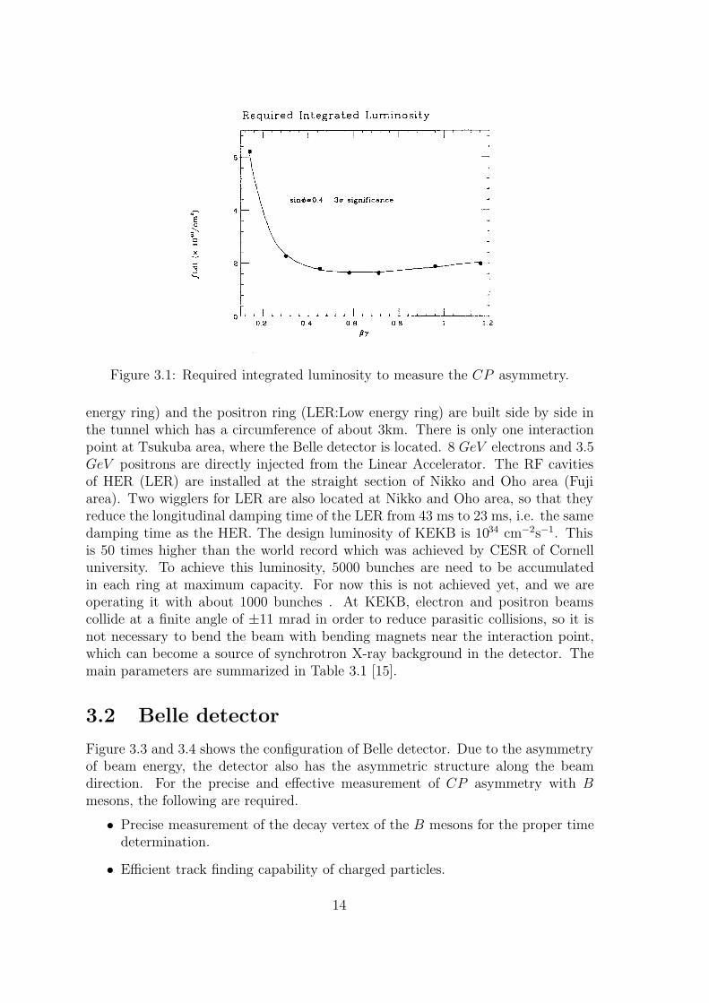
Figure 3.1: Required integrated luminosity to measure the CP asymmetry.
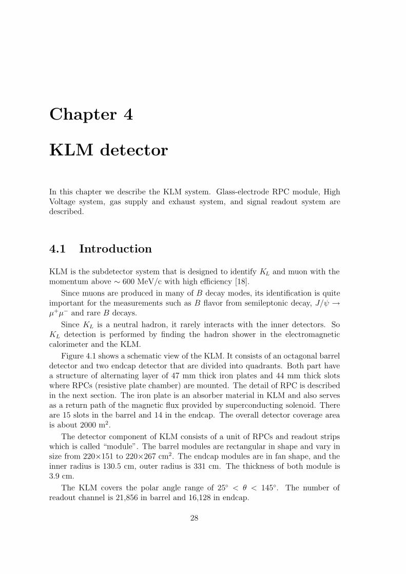
energy ring) and the positron ring (LER:Low energy ring) are built side by side inthe tunnel which has a circumference of about 3km. There is only one interactionpoint at Tsukuba area, where the Belle detector is located. 8 GeV electrons and 3.5GeV positrons are directly injected from the Linear Accelerator. The RF cavitiesof HER (LER) are installed at the straight section of Nikko and Oho area (Fujiarea). Two wigglers for LER are also located at Nikko and Oho area, so that theyreduce the longitudinal damping time of the LER from 43 ms to 23 ms, i.e. the samedamping time as the HER. The design luminosity of KEKB is 1034 cm−2s−1. Thisis 50 times higher than the world record which was achieved by CESR of Cornelluniversity. To achieve this luminosity, 5000 bunches are need to be accumulatedin each ring at maximum capacity. For now this is not achieved yet, and we areoperating it with about 1000 bunches . At KEKB, electron and positron beamscollide at a finite angle of ±11 mrad in order to reduce parasitic collisions, so it isnot necessary to bend the beam with bending magnets near the interaction point,which can become a source of synchrotron X-ray background in the detector. Themain parameters are summarized in Table 3.1 [15].
3.2 Belle detector
Figure 3.3 and 3.4 shows the configuration of Belle detector. Due to the asymmetryof beam energy, the detector also has the asymmetric structure along the beamdirection. For the precise and effective measurement of CP asymmetry with Bmesons, the following are required.
• Precise measurement of the decay vertex of the B mesons for the proper timedetermination.
• Efficient track finding capability of charged particles.
14
RF
RF
(Belle detector)
RF
RFRF
RF
Figure 3.2: Configuration of KEKB accelerator.
15
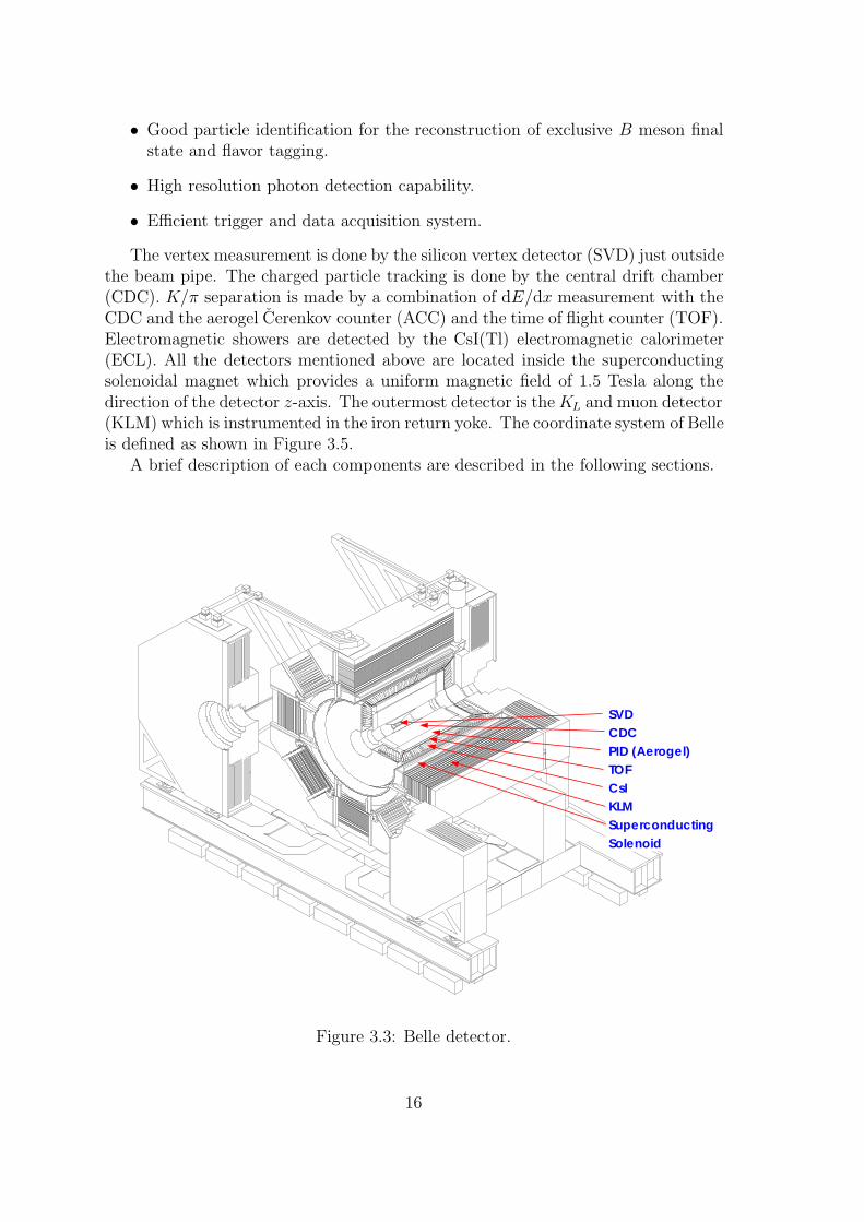
• Good particle identification for the reconstruction of exclusive B meson finalstate and flavor tagging.
• High resolution photon detection capability.
• Efficient trigger and data acquisition system.
The vertex measurement is done by the silicon vertex detector (SVD) just outsidethe beam pipe. The charged particle tracking is done by the central drift chamber(CDC). K/π separation is made by a combination of dE/dx measurement with theCDC and the aerogel Cerenkov counter (ACC) and the time of flight counter (TOF).Electromagnetic showers are detected by the CsI(Tl) electromagnetic calorimeter(ECL). All the detectors mentioned above are located inside the superconductingsolenoidal magnet which provides a uniform magnetic field of 1.5 Tesla along thedirection of the detector z-axis. The outermost detector is theKL and muon detector(KLM) which is instrumented in the iron return yoke. The coordinate system of Belleis defined as shown in Figure 3.5.
A brief description of each components are described in the following sections.
SVDCDCPID (Aerogel)TOFCsIKLM
SuperconductingSolenoid
Figure 3.3: Belle detector.
16
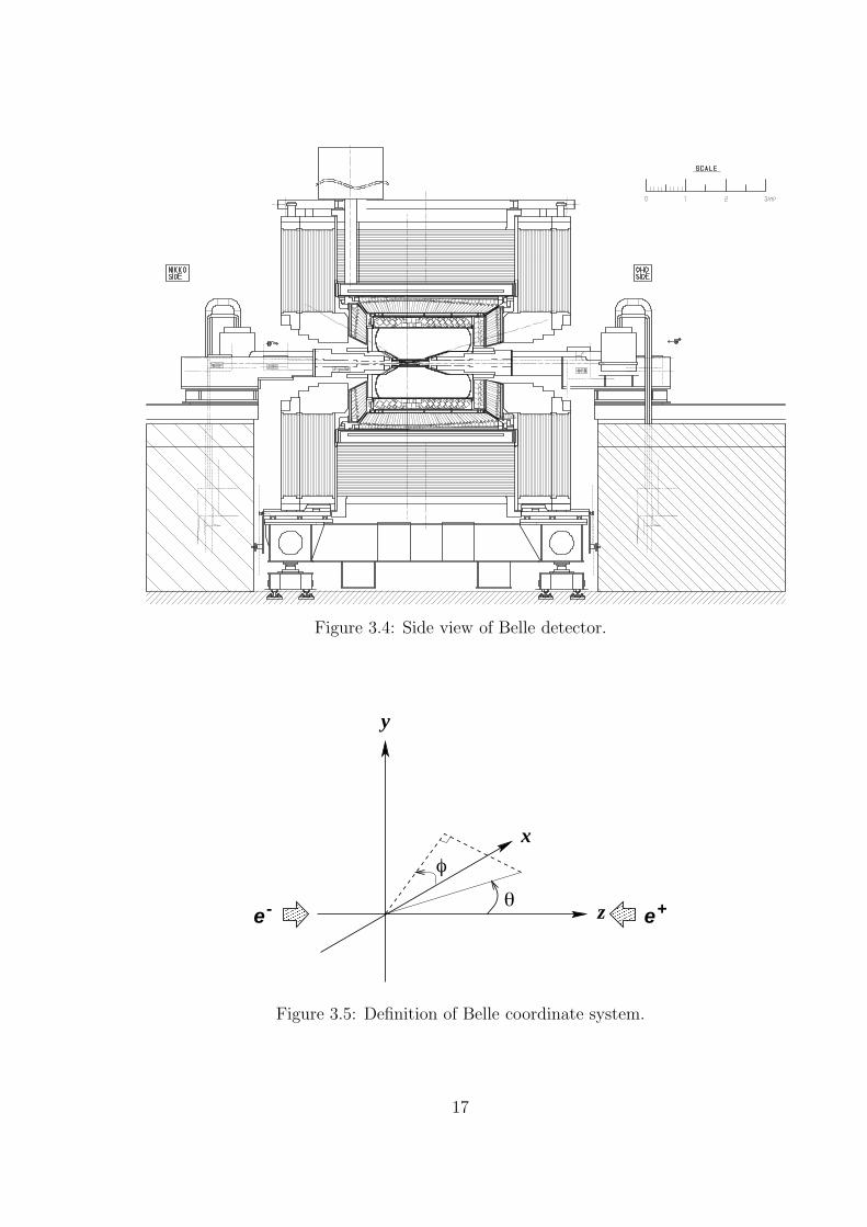
Figure 3.4: Side view of Belle detector.
z
x
φ
θ
y
e- e+
Figure 3.5: Definition of Belle coordinate system.
17
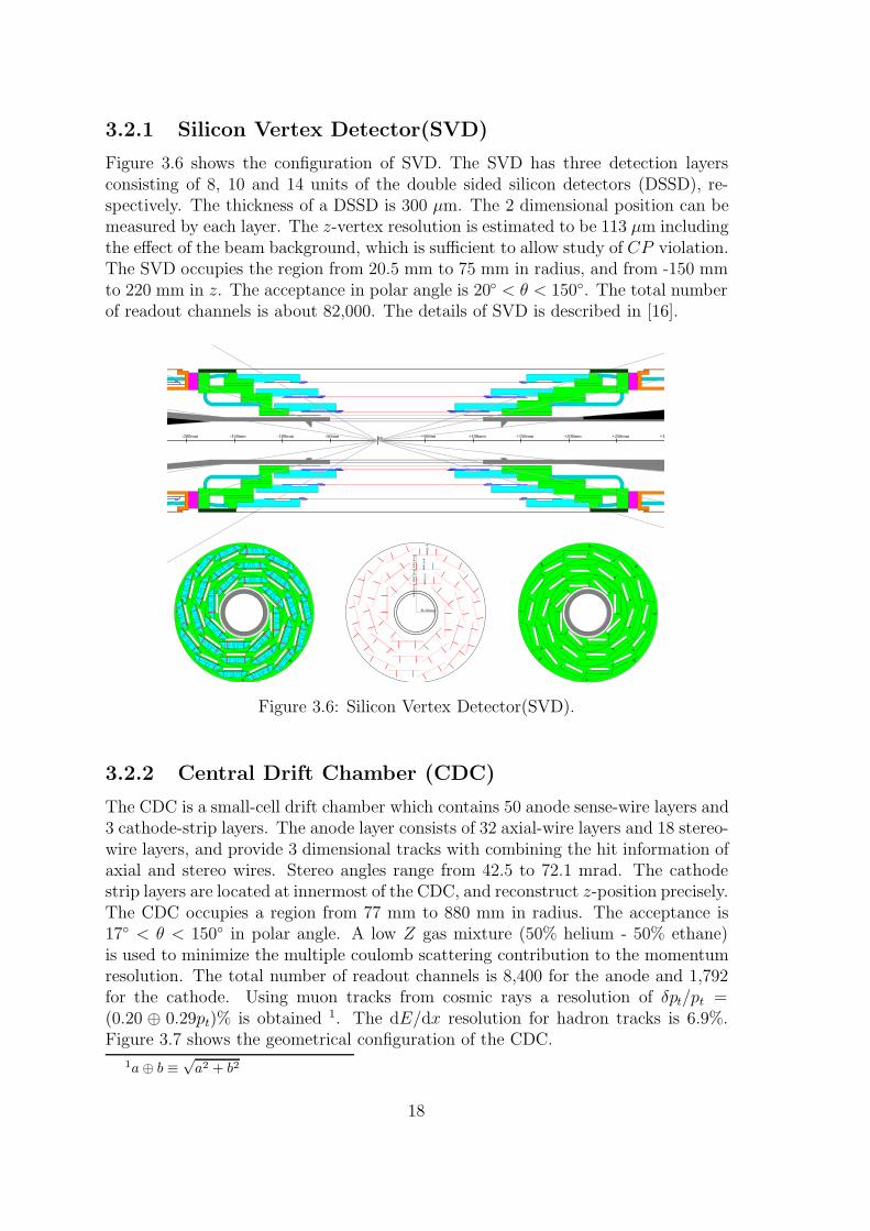
3.2.1 Silicon Vertex Detector(SVD)
Figure 3.6 shows the configuration of SVD. The SVD has three detection layersconsisting of 8, 10 and 14 units of the double sided silicon detectors (DSSD), re-spectively. The thickness of a DSSD is 300 µm. The 2 dimensional position can bemeasured by each layer. The z-vertex resolution is estimated to be 113 µm includingthe effect of the beam background, which is sufficient to allow study of CP violation.The SVD occupies the region from 20.5 mm to 75 mm in radius, and from -150 mmto 220 mm in z. The acceptance in polar angle is 20 < θ < 150. The total numberof readout channels is about 82,000. The details of SVD is described in [16].
IP +50mm +100mm +150mm +200mm +250mm +3-50mm-100mm-150mm-200mm
R=20mm
R=
30.0mm
R=
45.5mm
R=
60.5mm
d=9.5m
md=
8.5mm
d=12m
m
12
3
4
5
6
7
8
1
2
3
4
45
6
7
88 1
1
2
2
3
3
4
55
6
6
7
7
8
12
3
4
5
6
7
8
1
2
3
4
5
6
7
8
1
2
3
4
45
6
7
8
811
2
2
3
3
4
55
6
6
7
7
8
1
2
3
4
5
6
7
8
Figure 3.6: Silicon Vertex Detector(SVD).
3.2.2 Central Drift Chamber (CDC)
The CDC is a small-cell drift chamber which contains 50 anode sense-wire layers and3 cathode-strip layers. The anode layer consists of 32 axial-wire layers and 18 stereo-wire layers, and provide 3 dimensional tracks with combining the hit information ofaxial and stereo wires. Stereo angles range from 42.5 to 72.1 mrad. The cathodestrip layers are located at innermost of the CDC, and reconstruct z-position precisely.The CDC occupies a region from 77 mm to 880 mm in radius. The acceptance is17 < θ < 150 in polar angle. A low Z gas mixture (50% helium - 50% ethane)is used to minimize the multiple coulomb scattering contribution to the momentumresolution. The total number of readout channels is 8,400 for the anode and 1,792for the cathode. Using muon tracks from cosmic rays a resolution of δpt/pt =(0.20 ⊕ 0.29pt)% is obtained 1. The dE/dx resolution for hadron tracks is 6.9%.Figure 3.7 shows the geometrical configuration of the CDC.
1a ⊕ b ≡ √a2 + b2
18
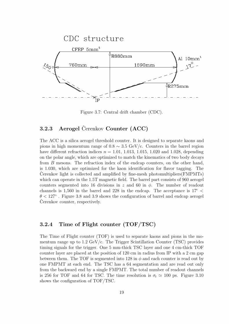
Figure 3.7: Central drift chamber (CDC).
3.2.3 Aerogel Cerenkov Counter (ACC)
The ACC is a silica aerogel threshold counter. It is designed to separate kaons andpions in high momentum range of 0.8 ∼ 3.5 GeV/c. Counters in the barrel regionhave different refraction indices n = 1.01, 1.013, 1.015, 1.020 and 1.028, dependingon the polar angle, which are optimized to match the kinematics of two body decaysfrom B mesons. The refraction index of the endcap counters, on the other hand,is 1.030, which are optimized for the kaon identification for flavor tagging. TheCerenkov light is collected and amplified by fine-mesh photomultipliers(FMPMTs)which can operate in the 1.5T magnetic field. The barrel part consists of 960 aerogelcounters segmented into 16 divisions in z and 60 in φ. The number of readoutchannels is 1,560 in the barrel and 228 in the endcap. The acceptance is 17 <θ < 127 . Figure 3.8 and 3.9 shows the configuration of barrel and endcap aerogelCerenkov counter, respectively.
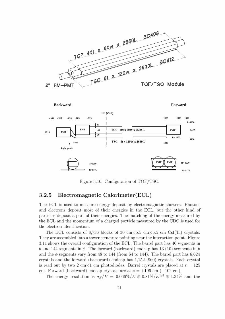
3.2.4 Time of Flight counter (TOF/TSC)
The Time of Flight counter (TOF) is used to separate kaons and pions in the mo-mentum range up to 1.2 GeV/c. The Trigger Scintillation Counter (TSC) providestiming signals for the trigger. One 5 mm-thick TSC layer and one 4 cm-thick TOFcounter layer are placed at the position of 120 cm in radius from IP with a 2 cm gapbetween them. The TOF is segmented into 128 in φ and each counter is read out byone FMPMT at each end. The TSC has a 64 segmentation and are read out onlyfrom the backward end by a single FMPMT. The total number of readout channelsis 256 for TOF and 64 for TSC. The time resolution is σt 100 ps. Figure 3.10shows the configuration of TOF/TSC.
19
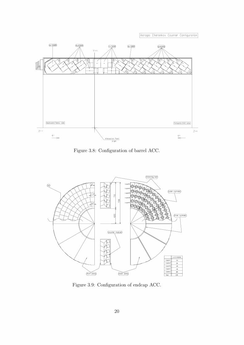
Figure 3.8: Configuration of barrel ACC.
Figure 3.9: Configuration of endcap ACC.
20
TSC 5t x 120W x 2630 L
PMT
20
1220
1825 1905
R= 1175
R=1250
1170
R= 1220R=1210
1930
R= 1175R=1175
PMT PMT
- 725 - 805- 835- 915- 940
1210
Light guide
TOF 40t x 60W x 2550 L
10
PMTPMT
ForwardBackward
1815- 815
40
I.P (Z=0)
Figure 3.10: Configuration of TOF/TSC.
3.2.5 Electromagnetic Calorimeter(ECL)
The ECL is used to measure energy deposit by electromagnetic showers. Photonsand electrons deposit most of their energies in the ECL, but the other kind ofparticles deposit a part of their energies. The matching of the energy measured bythe ECL and the momentum of a charged particle measured by the CDC is used forthe electron identification.
The ECL consists of 8,736 blocks of 30 cm×5.5 cm×5.5 cm CsI(Tl) crystals.They are assembled into a tower structure pointing near the interaction point. Figure3.11 shows the overall configuration of the ECL. The barrel part has 46 segments inθ and 144 segments in φ. The forward (backward) endcap has 13 (10) segments in θand the φ segments vary from 48 to 144 (from 64 to 144). The barrel part has 6,624crystals and the forward (backward) endcap has 1,152 (960) crystals. Each crystalis read out by two 2 cm×1 cm photodiodes. Barrel crystals are placed at r = 125cm. Forward (backward) endcap crystals are at z = +196 cm (−102 cm).
The energy resolution is σE/E = 0.066%/E ⊕ 0.81%/E1/4 ⊕ 1.34% and the
21
position resolution is σpos = 0.5 cm/√E, where the unit of E is GeV. Total amount
of material in front of the CsI is 0.387X0 at θ = 90, where X0 is the unit radiationlength.
3.2.6 KL/µ detector (KLM)
The KLM is the only sub-detector that is placed outside the solenoid coil. It wasdesigned to detect KL and muon. It consists of octagonal barrel region and twoendcap regions that are divided into quadrants. Both parts have a structure ofalternating layers of 47mm thick iron plates and 44mm thick slots where RPCs(Resistive plate chamber) are mounted. There are 15 slots in the barrel and 14 inthe endcap. The iron also serves as a flux return for the magnetic field of solenoidcoil.
The details of KLM is explained in chapter 4.
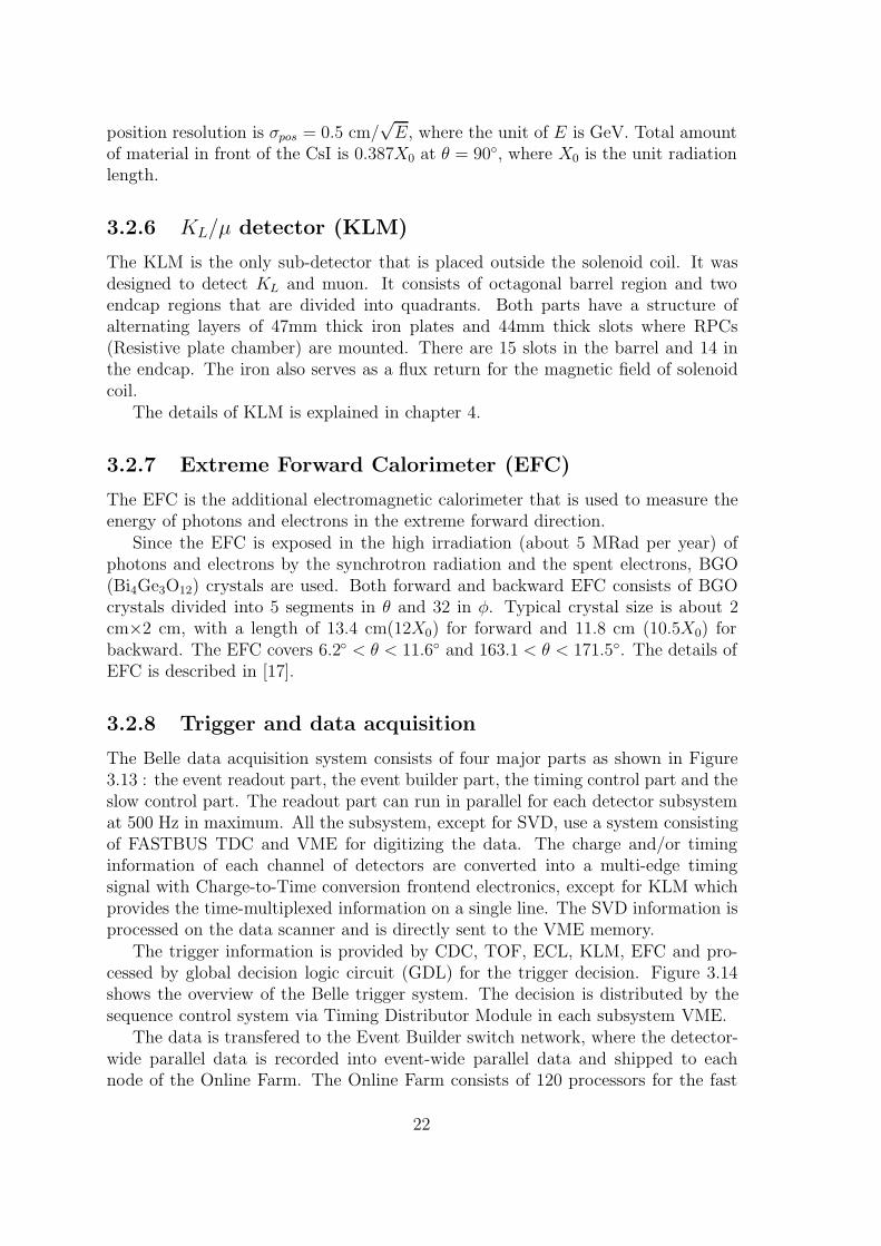
3.2.7 Extreme Forward Calorimeter (EFC)
The EFC is the additional electromagnetic calorimeter that is used to measure theenergy of photons and electrons in the extreme forward direction.
Since the EFC is exposed in the high irradiation (about 5 MRad per year) ofphotons and electrons by the synchrotron radiation and the spent electrons, BGO(Bi4Ge3O12) crystals are used. Both forward and backward EFC consists of BGOcrystals divided into 5 segments in θ and 32 in φ. Typical crystal size is about 2cm×2 cm, with a length of 13.4 cm(12X0) for forward and 11.8 cm (10.5X0) forbackward. The EFC covers 6.2 < θ < 11.6 and 163.1 < θ < 171.5. The details ofEFC is described in [17].
3.2.8 Trigger and data acquisition
The Belle data acquisition system consists of four major parts as shown in Figure3.13 : the event readout part, the event builder part, the timing control part and theslow control part. The readout part can run in parallel for each detector subsystemat 500 Hz in maximum. All the subsystem, except for SVD, use a system consistingof FASTBUS TDC and VME for digitizing the data. The charge and/or timinginformation of each channel of detectors are converted into a multi-edge timingsignal with Charge-to-Time conversion frontend electronics, except for KLM whichprovides the time-multiplexed information on a single line. The SVD information isprocessed on the data scanner and is directly sent to the VME memory.
The trigger information is provided by CDC, TOF, ECL, KLM, EFC and pro-cessed by global decision logic circuit (GDL) for the trigger decision. Figure 3.14shows the overview of the Belle trigger system. The decision is distributed by thesequence control system via Timing Distributor Module in each subsystem VME.
The data is transfered to the Event Builder switch network, where the detector-wide parallel data is recorded into event-wide parallel data and shipped to eachnode of the Online Farm. The Online Farm consists of 120 processors for the fast
22

Figure 3.11: CsI calorimeter.
23
Figure 3.12: Extreme Forward Calorimeter.
reconstruction of up to 15 MBytes/sec event data stream. The events which passedthe Farm is stored into the Mass Storage System and eventually stored into the tapesystem.
All the subsystem are controlled centrally by the Master Control. The messagepassing is done through a conventional TCP/IP network. The network also providesan experiment-wide shared memory (NSM) in order to store the useful run-relatedand environmental-related information for control and monitoring purpose.
3.3 KEKB and Belle commissioning
The detector construction was completed in Dec.1998. The detector has been cali-brated with cosmic rays. The first cosmic ray event was observed on Jan.18, 1999with all the subsystems operating with and without 1.5 Tesla magnetic field. Thedetector was rolled into the interaction point on May 1, 1999.
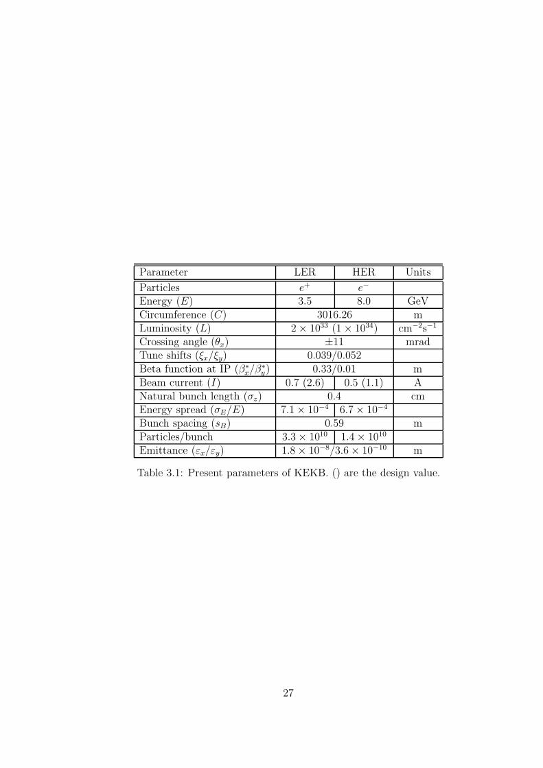
The first commissioning of the KEKB accelerator was from May 24 to Aug.4,1999. The first B meson was observed on Jun.1, 1999. During first beam run period,the peak luminosity reached 3×1032cm−2s−1, and 26 pb−1 data were recorded in total.During the running from Oct., 1999 to July, 2000, the peak luminosity has reached2.2× 1033cm−2s−1, and the integrated luminosity of 6.8 fb−1 was accumulated. Thepresent peak luminosity is still 20% of the designed value. Efforts for further machinetuning and improvement of some of the machine components continue. Figure 3.15
24
VME
MPX
Q/T TDC VME
Q/T TDC VME
Q/T TDC VME
Q/T TDC VME
TDC VME
Q/T TDC VMEMasterControl
Unit
HVMonitor
& Control
Monitor& Alarm
AcceleratorComm.
EventBuilder
OnlineComputer
Farm
MassStorageSystem
TriggerDecision
LogicData ScannerSVD
CDC
ACC
TOF
ECL
KLM
EFC
Backgr.Monitor
LuminosityMonitor
SequenceControl
Unit
Detector Subsystems
Data flow
Control flow
Timing signal
Timing signal
Control Control
Figure 3.13: Data acquisition system.
SVD
CDC
TSC
ECL
Timing
>
Glo
bal D
ecis
ion
Logi
c
Trigger SignalGate/Stop
2.2 µsec after event crossing
Rφ Track Topology
Stereo Wires
Cathod Pads
Z Track
Beam Crossing
Belle Trigger System
Rφ
Z
Hit
4x4 Sum Cluster Count
Threshold
EFC Amp. Bhabha Logic
Two γ Logic
KLM Hit
Track Segment
Z Finder
Rφ Track
Z Track
TSC Trigger
Low Threshold
High Threshold
E Sum
Low Threshold
High Threshold
µ hit
Combined Track
Cluster Count
Axial Wires
Figure 3.14: Trigger scheme.
25
shows the history of the luminosity of the KEKB until July 2000.
Figure 3.15: History of integrated luminosity of KEKB.
26
Parameter LER HER Units
Particles e+ e−
Energy (E) 3.5 8.0 GeVCircumference (C) 3016.26 mLuminosity (L) 2 × 1033 (1 × 1034) cm−2s−1
Crossing angle (θx) ±11 mradTune shifts (ξx/ξy) 0.039/0.052Beta function at IP (β∗
x/β∗y) 0.33/0.01 m
Beam current (I) 0.7 (2.6) 0.5 (1.1) ANatural bunch length (σz) 0.4 cmEnergy spread (σE/E) 7.1 × 10⁻⁴ 6.7 × 10⁻⁴
Bunch spacing (sB) 0.59 mParticles/bunch 3.3 × 10¹⁰ 1.4 × 10¹⁰
Emittance (εx/εy) 1.8 × 10⁻⁸/3.6 × 10−10 m
Table 3.1: Present parameters of KEKB. () are the design value.
27
Chapter 4
KLM detector
In this chapter we describe the KLM system. Glass-electrode RPC module, HighVoltage system, gas supply and exhaust system, and signal readout system aredescribed.
4.1 Introduction
KLM is the subdetector system that is designed to identify KL and muon with themomentum above ∼ 600 MeV/c with high efficiency [18].
Since muons are produced in many of B decay modes, its identification is quiteimportant for the measurements such as B flavor from semileptonic decay, J/ψ →µ+µ− and rare B decays.
Since KL is a neutral hadron, it rarely interacts with the inner detectors. SoKL detection is performed by finding the hadron shower in the electromagneticcalorimeter and the KLM.
Figure 4.1 shows a schematic view of the KLM. It consists of an octagonal barreldetector and two endcap detector that are divided into quadrants. Both part havea structure of alternating layer of 47 mm thick iron plates and 44 mm thick slotswhere RPCs (resistive plate chamber) are mounted. The detail of RPC is describedin the next section. The iron plate is an absorber material in KLM and also servesas a return path of the magnetic flux provided by superconducting solenoid. Thereare 15 slots in the barrel and 14 in the endcap. The overall detector coverage areais about 2000 m2.
The detector component of KLM consists of a unit of RPCs and readout stripswhich is called “module”. The barrel modules are rectangular in shape and vary insize from 220×151 to 220×267 cm2. The endcap modules are in fan shape, and theinner radius is 130.5 cm, outer radius is 331 cm. The thickness of both module is3.9 cm.
The KLM covers the polar angle range of 25 < θ < 145. The number ofreadout channel is 21,856 in barrel and 16,128 in endcap.
28
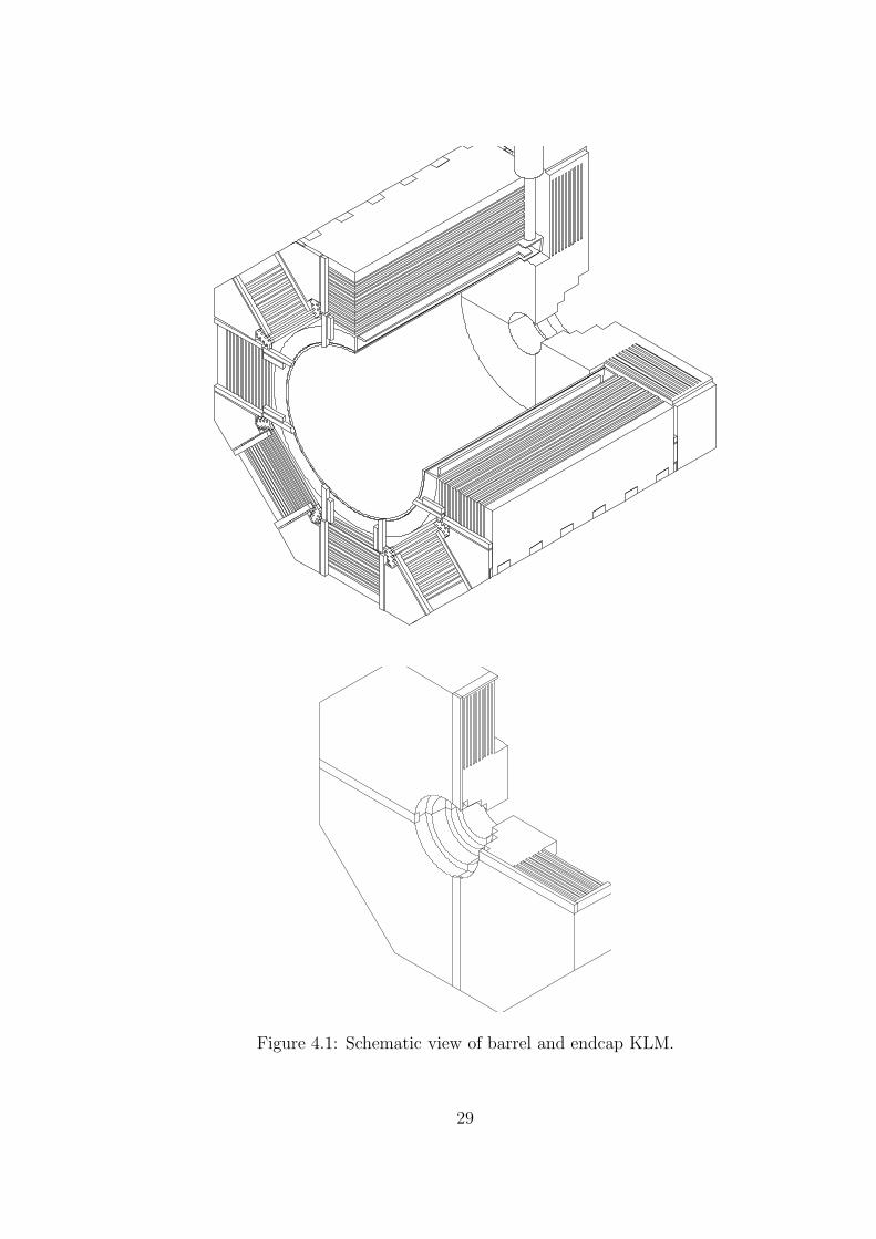
Figure 4.1: Schematic view of barrel and endcap KLM.
29
4.2 Glass-electrode RPC
The RPC is essentially like a planer spark counter wherein the avalanche inducedby an incident charged particle is quenched when the limited amount of charge onthe inner surface of high resistive electrodes is exhausted.
The RPC has features as follows.
• Signal pulse height is high (∼ several 100 mV) enough to operate withoutamplifier.
• Good time resolution (∼ several nsec).
• Easy to build. Have freedom in size and shape.
• Not so expensive.
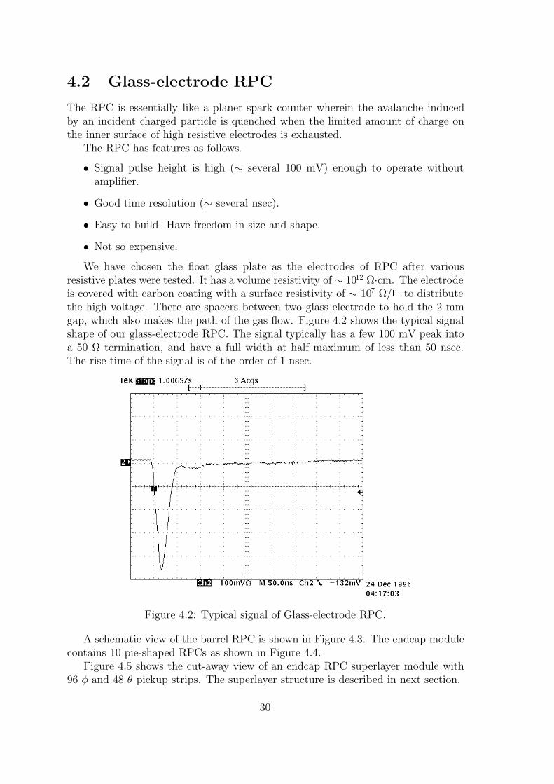
We have chosen the float glass plate as the electrodes of RPC after variousresistive plates were tested. It has a volume resistivity of ∼ 1012 Ω·cm. The electrodeis covered with carbon coating with a surface resistivity of ∼ 107 Ω/ to distributethe high voltage. There are spacers between two glass electrode to hold the 2 mmgap, which also makes the path of the gas flow. Figure 4.2 shows the typical signalshape of our glass-electrode RPC. The signal typically has a few 100 mV peak intoa 50 Ω termination, and have a full width at half maximum of less than 50 nsec.The rise-time of the signal is of the order of 1 nsec.
Figure 4.2: Typical signal of Glass-electrode RPC.
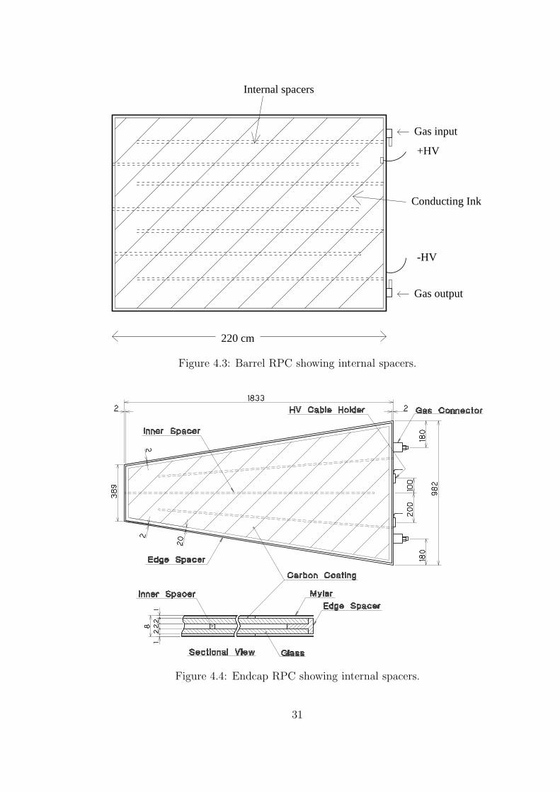
A schematic view of the barrel RPC is shown in Figure 4.3. The endcap modulecontains 10 pie-shaped RPCs as shown in Figure 4.4.
Figure 4.5 shows the cut-away view of an endcap RPC superlayer module with96 φ and 48 θ pickup strips. The superlayer structure is described in next section.
30
Gas output
220 cm
+HV
-HV
Internal spacers
Conducting Ink
Gas input
Figure 4.3: Barrel RPC showing internal spacers.
Figure 4.4: Endcap RPC showing internal spacers.
31
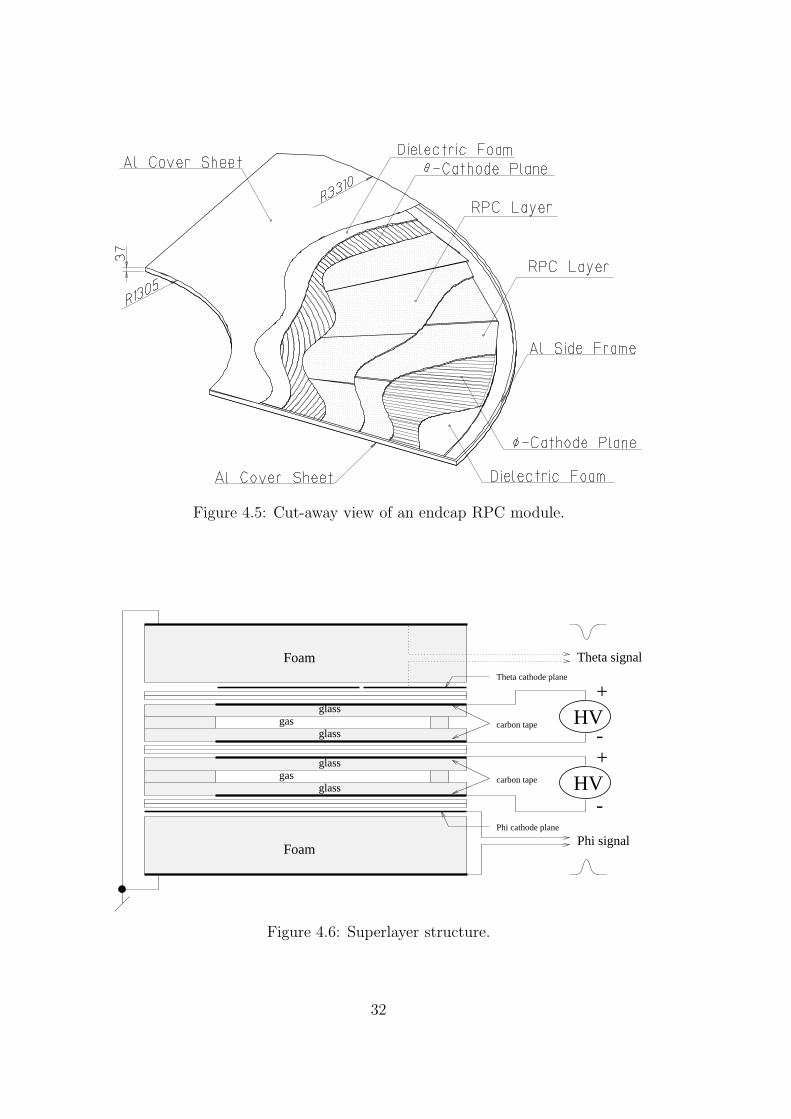
Figure 4.5: Cut-away view of an endcap RPC module.
glass
glass
gas
gasglass
glass
Foam
FoamPhi signal
Theta signal
Phi cathode plane
carbon tape
carbon tape
Theta cathode plane
+
-HV
+
-HV
Figure 4.6: Superlayer structure.
32

4.3 Superlayer structure
The superlayer structure consist of two RPCs sandwiched between orthogonal pickupstrip planes as shown in Figure 4.6. The HV is supplied to the same direction fortwo RPC layers so that both readout planes could produce signals when either RPCfires. This design minimizes the effect of dead regions between gaps in adjacentRPCs and near the internal spacers by offsetting their locations for two RPCs thatcomprise a superlayer, which result in a high efficiency.
4.4 Gas system
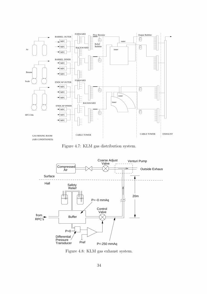
We have chosen the gas mixture of 30% argon, 62% HFC134a, and 8% butane-silver(iso-/n-∼25/75), which is environmentally friendly and non-flammable andprovides high detection efficiency and stable RPC operation[19].
Figure 4.7 shows the block diagram of the KLM gas distribution. Mixed gas issupplied to each RPC in a superlayer so that if one supply line fails the other willstill be operational. To insure the uniform gas distribution for 704 channel, “FlowRegisters” which is a 10 cm long stainless steel tube of 254 µm diameter are insertedupstream of the RPC. Since mixed gas is heavier than air, the gas, that fills the 20m vertical exhaust line to the ground level, exerts about 40 mmAq pressure to theRPCs, which might damage them. We use Venturi pump to control the exhaustpressure differential to be nearly zero. The exhaust system is shown in Figure 4.8.
During initial operation, we experienced a damage of the electrode surface whichis caused by water vapor. We found it from the increase of dark current and corre-sponding decrease of efficiency. The water vapor was migrating through the poly-olefin tubings, and the concentration of H2O was measured to be about 2000 ppmin some exhaust lines. By replacing the polyolefin tubing with copper tubing, thecontaminated RPCs eventually dried out and have recovered the efficiency. Nowcareful control and monitor of water vapor in the gas are made by the water filtersand dew point meters. Interlock system turns off the HV to protect the glass surfaceif abnormal gas mixture is detected.
4.5 HV system
RPCs are operated in a limited streamer mode. Applied high voltage is fixed to +4.7(+4.5) kV for anode plane of barrel (endcap) RPCs and −3.5 kV for cathode planefor barrel and endcap RPCs. Dark current of individual layer is carefully monitoredsince efficiency becomes lower when the current exceeds the nominal value of ∼ 7µA per one RPC layer.
33
MFC
MFC
MFC
MFC
MFC
MFC
MFC
MFC
MFC
MFC
MFC
MFC
Ar
Butane
Scale
HFC134a
ReliefBubbler
Flow Resistor
outer
inner
outer
inner
Output Bubbler
GAS MIXING ROOM
(AIR CONDITIONED)
CABLE TOWER CABLE TOWER EXHAUST
BARREL OUTER
BARREL INNER
ENDCAP OUTER
ENDCAP INNER
FORWARD
BACKWARD
FORWARD
BACKWARD
Figure 4.7: KLM gas distribution system.
Relief
fromRPC’s
P=-250 mmAq
Safety
P=~0 mmAq
Hall
Surface
Coarse Adjust
20m
Transducer
Outside Exhaust
Venturi Pump
PrefPressureDifferential
Control
Buffer
P=0
Valve
AirCompressed
Valve
Figure 4.8: KLM gas exhaust system.
34
4.6 Readout system
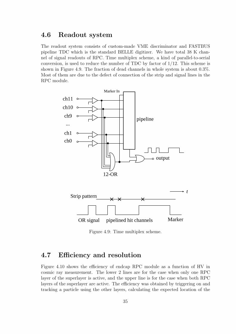
The readout system consists of custom-made VME discriminator and FASTBUSpipeline TDC which is the standard BELLE digitizer. We have total 38 K chan-nel of signal readouts of RPC. Time multiplex scheme, a kind of parallel-to-serialconversion, is used to reduce the number of TDC by factor of 1/12. This scheme isshown in Figure 4.9. The fraction of dead channels in whole system is about 0.3%.Most of them are due to the defect of connection of the strip and signal lines in theRPC module.
ch11
ch10
ch9
ch1
ch0
pipeline...
12-OR
output
Marker In
OR signal pipelined hit channels Marker
tStrip pattern
Figure 4.9: Time multiplex scheme.
4.7 Efficiency and resolution
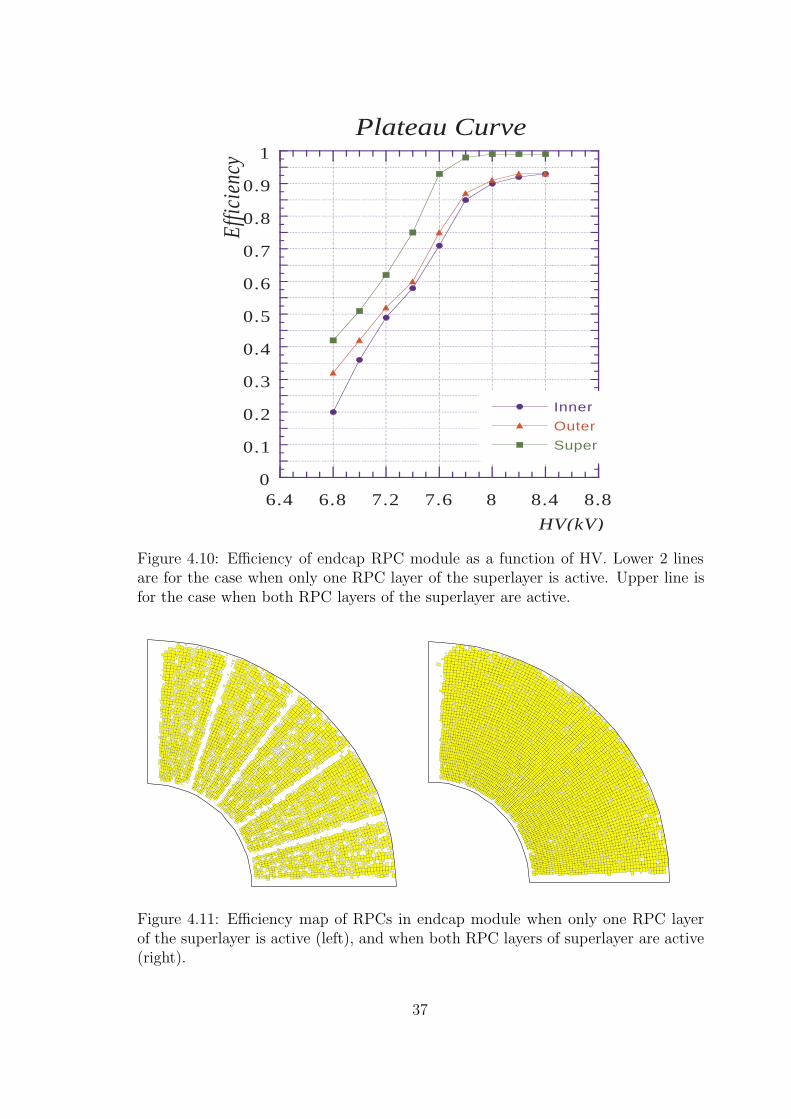
Figure 4.10 shows the efficiency of endcap RPC module as a function of HV incosmic ray measurement. The lower 2 lines are for the case when only one RPClayer of the superlayer is active, and the upper line is for the case when both RPClayers of the superlayer are active. The efficiency was obtained by triggering on andtracking a particle using the other layers, calculating the expected location of the
35

track as it passed through this layer, and looking to see if a hit was recorded at thatlocation (±1 strip). The efficiency is the ratio of the number of hits found to thenumber expected. Figure 4.11 shows the efficiency map with a grid determined bythe readout strip. The size of the box indicates the efficiency of the grid. When onlyone RPC layer of the superlayer is active, the edges of each RPC and the regionnear the internal spacers are clearly seen as inefficient regions. When both RPClayer are active, the superlayer acts as a logical “OR” for hits of either RPC layer.Since care was taken to insure that the edges of RPCs in the two RPC layers do notoverlap, we obtain the uniform efficiency that is typically over 98%.
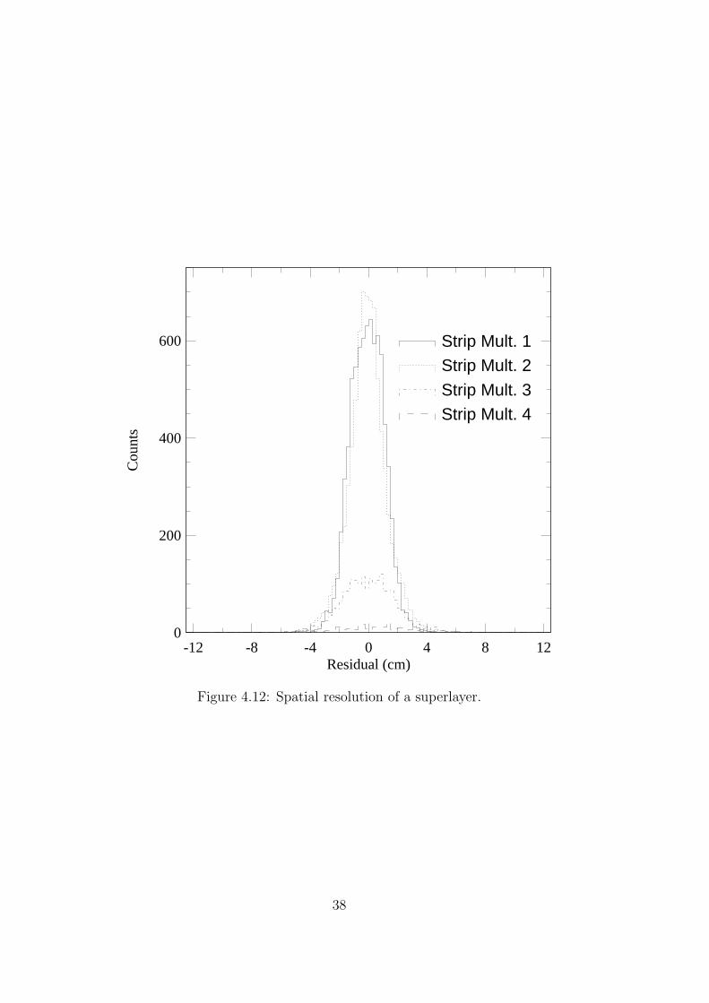
Figure 4.12 shows the spatial resolution of the modules. This residual distri-bution shows the difference between the measured and predicted hit location usingthe track that has been fitted using hits in the adjacent layers. The multiplicityreferred to is the number of adjacent strips that produces signal. When this stripmultiplicity is more than one, the hit location is determined as the center of thestrips. With one or two strips hit the standard deviation is 1.1cm. With three hitstrips it is 1.7cm, and with four hit strips it is 2.9cm. The multiplicity-weightedstandard-deviation is 1.2cm, which gives the angular resolution from the interactionpoint better than 10 mrad. The resolution is almost the same as that expected fromstrip size and assumption of uniform distribution of particles.
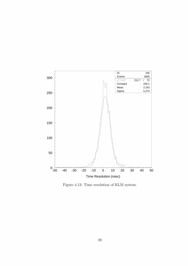
Figure 4.13 shows the ∆t distribution of 2 KLM layers using cosmic lays. Thetime resolution of the KLM system is ∼ several nsec.
36
0
0.1
0.2
0.3
0.4
0.5
0.6
0.7
0.8
0.9
1
6.4 6.8 7.2 7.6 8 8.4 8.8
Plateau Curve
Inner
Outer
Super
Effic
ienc
y
HV(kV)
Figure 4.10: Efficiency of endcap RPC module as a function of HV. Lower 2 linesare for the case when only one RPC layer of the superlayer is active. Upper line isfor the case when both RPC layers of the superlayer are active.
Figure 4.11: Efficiency map of RPCs in endcap module when only one RPC layerof the superlayer is active (left), and when both RPC layers of superlayer are active(right).
37
-12 -8 -4 0 4 8 12Residual (cm)
0
200
400
600
Cou
nts
Strip Mult. 1Strip Mult. 2
Strip Mult. 3Strip Mult. 4
Figure 4.12: Spatial resolution of a superlayer.
38
0
50
100
150
200
250
300
-50 -40 -30 -20 -10 0 10 20 30 40 50
Time Resolution (nsec)
IDEntries
100 3605
212.7 / 72
Constant 239.1
Mean 2.243Sigma 5.274
Figure 4.13: Time resolution of KLM system.
39
Chapter 5
Software Tools
In this chapter we describe the software tools for data analysis and for Monte Carlosimulation of the Belle detector.
5.1 Overview
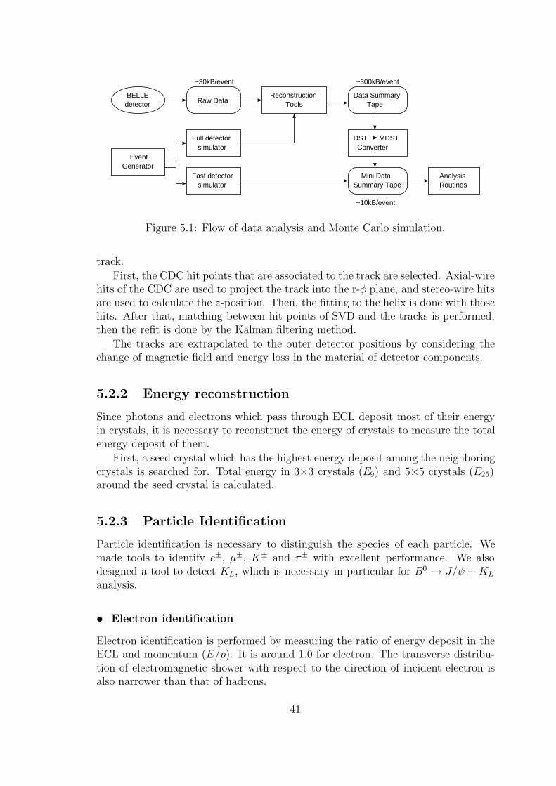
Figure 5.1 shows the general framework of data analysis and Monte Carlo simulationin the Belle experiment. The raw data taken by the Belle DAQ are processed byreconstruction tools, such as charged particle tracker, energy measurement and par-ticle identifications. Output of reconstruction tools are stored into Data SummaryTape (DST). For physics analysis, DSTs are converted to the more convenient andcompact subset of data, so-called Mini-DST (MDST).
For Monte Carlo simulation, we have two detector simulator : full detector sim-ulator and fast detector simulator. The full detector simulator generates detectorresponse in the same way as the real detector generates it. Data generated by fulldetector simulator is processed by the reconstruction tools, and subsequent processis the same as in the real data. The fast detector simulator uses the parameterizeddetector performances, and generate Mini-DST data directly.
Analysis and simulation tools consist of many program modules which are exe-cuted on a common framework, BASF/FPDA [20]. Data are managed by the banksystem, PANTHER [21], which is based on entity relationship model [22]. PAN-THER can be used from either FORTRAN, C or C++ languages.
5.2 Reconstruction tools
For the event reconstruction for physics analysis, it is necessary to perform chargedparticle tracking, energy measurement and particle identification.
5.2.1 Charged particle tracking
The charged particle tracking tries to find all tracks in the event and reconstructthem, and provide the coordinate, momentum, energy deposit (dE/dx), for each
40
BELLEdetector Raw Data
Reconstruction Tools
Data Summary Tape
EventGenerator
Full detector simulator
Fast detector simulator
DST MDST Converter
Mini DataSummary Tape
AnalysisRoutines
~30kB/event ~300kB/event
~10kB/event
Figure 5.1: Flow of data analysis and Monte Carlo simulation.
track.
First, the CDC hit points that are associated to the track are selected. Axial-wirehits of the CDC are used to project the track into the r-φ plane, and stereo-wire hitsare used to calculate the z-position. Then, the fitting to the helix is done with thosehits. After that, matching between hit points of SVD and the tracks is performed,then the refit is done by the Kalman filtering method.
The tracks are extrapolated to the outer detector positions by considering thechange of magnetic field and energy loss in the material of detector components.
5.2.2 Energy reconstruction
Since photons and electrons which pass through ECL deposit most of their energyin crystals, it is necessary to reconstruct the energy of crystals to measure the totalenergy deposit of them.
First, a seed crystal which has the highest energy deposit among the neighboringcrystals is searched for. Total energy in 3×3 crystals (E9) and 5×5 crystals (E25)around the seed crystal is calculated.
5.2.3 Particle Identification
Particle identification is necessary to distinguish the species of each particle. Wemade tools to identify e±, µ±, K± and π± with excellent performance. We alsodesigned a tool to detect KL, which is necessary in particular for B0 → J/ψ +KL
analysis.
• Electron identification
Electron identification is performed by measuring the ratio of energy deposit in theECL and momentum (E/p). It is around 1.0 for electron. The transverse distribu-tion of electromagnetic shower with respect to the direction of incident electron isalso narrower than that of hadrons.
41
For electron identification, E/p is the main method. In addition to it, we usematching information of track and ECL cluster, shower shape, dE/dx in the CDC,light yield in the ACC, and time of flight measured by the TOF.
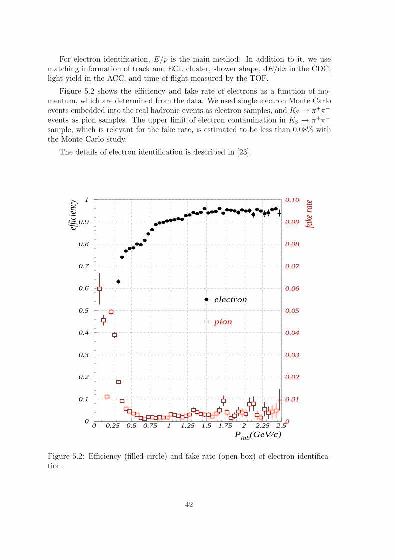
Figure 5.2 shows the efficiency and fake rate of electrons as a function of mo-mentum, which are determined from the data. We used single electron Monte Carloevents embedded into the real hadronic events as electron samples, and KS → π+π−
events as pion samples. The upper limit of electron contamination in KS → π+π−
sample, which is relevant for the fake rate, is estimated to be less than 0.08% withthe Monte Carlo study.
The details of electron identification is described in [23].
0
0.1
0.2
0.3
0.4
0.5
0.6
0.7
0.8
0.9
1
0 0.25 0.5 0.75 1 1.25 1.5 1.75 2 2.25 2.5
electron
pion
0
0.01
0.02
0.03
0.04
0.05
0.06
0.07
0.08
0.09
0.10
fake
rate
Plab(GeV/c)
effic
ienc
y
Figure 5.2: Efficiency (filled circle) and fake rate (open box) of electron identifica-tion.
42
• Muon identification
Muon is more penetrative than any other charged particle since muon is massiveand does not produce electromagnetic shower. Charged tracks are extrapolated toKLM region, then KLM hits nearby the track are collected. The track extrapolationis performed by Kalman filtering method inside the KLM region.
Use of hit information of the KLM is the main method for muon identification.The depth of KLM hits shows ∆R which is the difference between the measured andexpected range of track. The spread of KLM hits shows χ2
r which is the normalizedtransverse deviations of all hits associated with the track. Probability density dis-tributions of ∆R and χ2
r, obtained from Monte Carlo single track of muons, pionsand kaons, are used to calculate the likelihood.
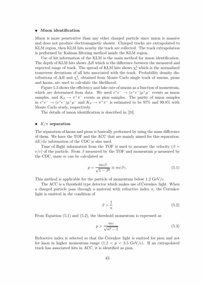
Figure 5.3 shows the efficiency and fake rate of muons as a function of momentum,which are determined from data. We used e+e− → (e+e−)µ+µ− events as muonsamples, and KS → π+π− events as pion samples. The purity of muon samplesin e+e− → (e+e−)µ+µ− and KS → π+π− is estimated to be 97% and 99.8% withMonte Carlo study, respectively.
The details of muon identification is described in [24].
• K/π separation
The separation of kaons and pions is basically performed by using the mass differenceof them. We have the TOF and the ACC that are mainly aimed for this separation.dE/dx information of the CDC is also used.
Time of flight information from the TOF is used to measure the velocity (β =v/c) of the particle. From β measured by the TOF and momentum p measured bythe CDC, mass m can be calculated as
p =mcβ√1 − β2
≡ mcβγ. (5.1)
This method is applicable for the particle of momentum below 1.2 GeV/c.The ACC is a threshold type detector which makes use of Cerenkov light. When
a charged particle pass through a material with refractive index n, the Cerenkovlight is emitted in the condition of
β >1
n(5.2)
From Equation (5.1) and (5.2), the threshold momentum is expressed as
p >mc√n2 − 1
(5.3)
Refractive index is selected so that the Cerenkov light is emitted for pion and notfor kaon in higher momentum range (1.2 < p < 3.5 GeV/c). If an extrapolatedtrack has associated hits in ACC, it is identified as pion.
43
0
0.1
0.2
0.3
0.4
0.5
0.6
0.7
0.8
0.9
1
0 0.25 0.5 0.75 1 1.25 1.5 1.75 2 2.25 2.5P(GeV/c)
effici
ency
0
0.01
0.02
0.03
0.04
0.05
0.06
0.07
0.08
0.09
0.1
fake
rate
Figure 5.3: Efficiency (filled circle) and fake rate (open circle) of muon identification.
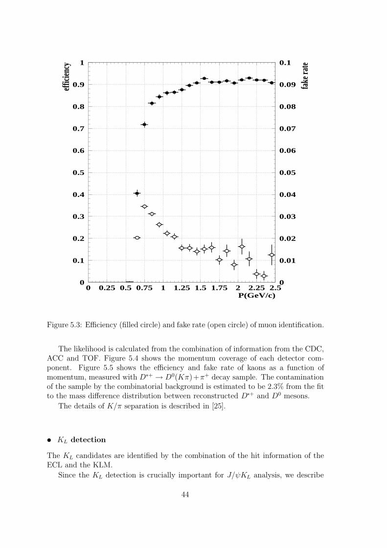
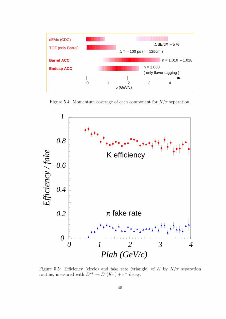
The likelihood is calculated from the combination of information from the CDC,ACC and TOF. Figure 5.4 shows the momentum coverage of each detector com-ponent. Figure 5.5 shows the efficiency and fake rate of kaons as a function ofmomentum, measured with D∗+ → D0(Kπ)+π+ decay sample. The contaminationof the sample by the combinatorial background is estimated to be 2.3% from the fitto the mass difference distribution between reconstructed D∗+ and D0 mesons.
The details of K/π separation is described in [25].
• KL detection
The KL candidates are identified by the combination of the hit information of theECL and the KLM.
Since the KL detection is crucially important for J/ψKL analysis, we describe
44
0 1 2 3 4p (GeV/c)
dE/dx (CDC)
TOF (only Barrel)
Barrel ACC
Endcap ACC
∆ dE/dX ∼ 5 %
∆ T ∼ 100 ps (r = 125cm )
n = 1.010 ∼ 1.028
n = 1.030( only flavor tagging )
Figure 5.4: Momentum coverage of each component for K/π separation.
0
0.2
0.4
0.6
0.8
1
0 1 2 3 4
K efficiency
π fake rate
Plab (GeV/c)
Eff
icie
ncy
/ fak
e
Figure 5.5: Efficiency (circle) and fake rate (triangle) of K by K/π separationroutine, measured with D∗+ → D0(Kπ) + π+ decay.
45
the details in the next chapter.
5.3 Monte Carlo simulation
Monte Carlo simulation is necessary to know the reconstruction efficiency and thebackground contamination.
5.3.1 Event generator
The event generator simulates the physical process of particle decay chain. Theinitial state is Υ(4S) or qq (for continuum) and the final states consist of stableparticles. We use QQ [26] event generator originally developed by CLEO group andmodified to match the Belle experiment [27]. QQ can handle either Υ(4S) decays orcontinuum process. The decay of particle is performed according to the decay tablewhich contains the decay modes and branching ratios measured by CLEO. User cancontrol decay mode of any particle by changing the decay table. The output of QQis stored into HEPEVT table [28] which includes production time, vertex position,4-momentum, decay subproducts, etc.
5.3.2 Full detector simulation
The full detector simulator is based on GEANT3 [29], which is a library developed atCERN to simulate the passage of particles through the materials. GEANT systemallows us to describe an experimental setup by a structure of geometrical volumes,and transport particles which are generated by an event generator through the var-ious ranges of the setup, taking into account geometrical volume boundaries andphysical effects according to the nature of particles themselves, their interactionswith matter and the magnetic field.
The full detector simulation takes long time to process (∼30 sec/event) since ittraces all particle step by step computing reactions with materials.
5.3.3 Fast detector simulation
The fast detector simulator was developed [30] to save processing time when wesimulate a large number of background events.
The fast detector simulation takes the particles from the event generator as aninput, and calculate the detector responses with smearing functions based on simpleparameterization. Some of the smearing functions are determined from full detectorsimulation, some are based on the results of the beam tests, and others are fromreal data if it is possible to use. The fast detector simulator produces the Mini-DSTformat output data directly. The fast detector simulator could not take into accountthe effect of secondary particles generated by the reaction of particles and detectormaterials.
46

Chapter 6
KL detection
In this chapter we describe the KL identification method and its performance withthe Belle detector.
6.1 KL selection criteria
The KL candidates are identified using the combination of the hit information ofthe ECL and the KLM. Following algorithm is used to select the KL candidates.
1. Hit clusters are made by combining nearby KLM hits which are within 5
opening angles each other. This process is repeated until no more hit is foundwithin 5 opening angle from each other. We call this hit cluster “KLM clus-ter”.
2. KLM clusters are classified as charged or neutral. Each charged track foundby inner tracker is extrapolated to the first layer of KLM, and the meetingpoint is joined to interaction point by a straight line. If this line is withinthe 15 cone around the KLM cluster direction, the KLM cluster is defined asbeing associated with the charged track, and is classified as charged cluster.Otherwise the cluster is classified as neutral cluster.
3. Calculate the direction of neutral KLM cluster for two different cases sepa-rately.
• If the neutral ECL shower with energy(EECL) greater than 0.16 GeV isfound within the 15 opening angle of the KLM cluster direction, theKLM cluster is said to be associated with the ECL shower, and we usethe direction of ECL shower as the direction of KLM cluster.
• If no ECL shower is found to associate to KLM cluster, we use the direc-tion of the center of KLM cluster as the direction of the KLM cluster.
4. KL candidates are required to satisfy following conditions.
• The KLM cluster is a neutral cluster.
47
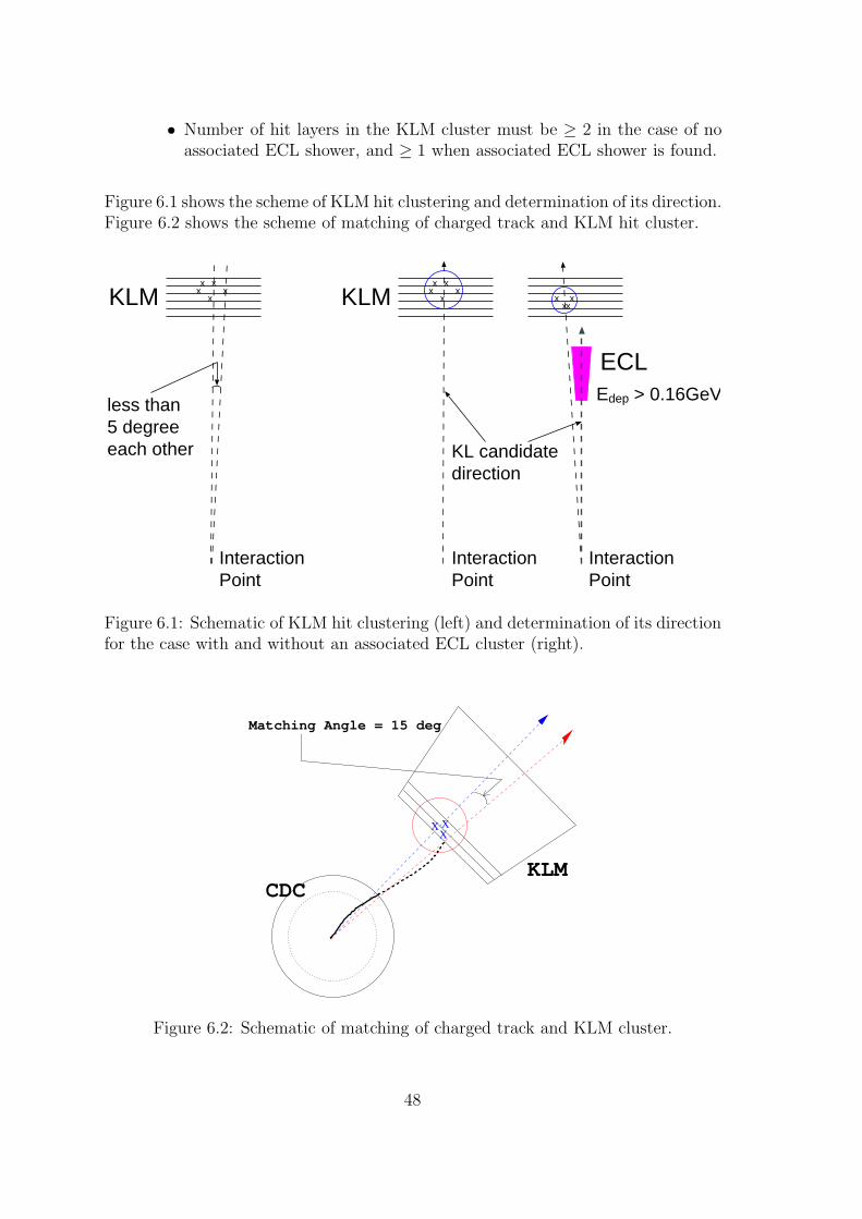
• Number of hit layers in the KLM cluster must be ≥ 2 in the case of noassociated ECL shower, and ≥ 1 when associated ECL shower is found.
Figure 6.1 shows the scheme of KLM hit clustering and determination of its direction.Figure 6.2 shows the scheme of matching of charged track and KLM hit cluster.
x
KLMx
x xx
InteractionPoint
x
KLMx
x xx
InteractionPoint
x xxx
less than5 degreeeach other
ECLE > 0.16GeVdep
InteractionPoint
KL candidatedirection
Figure 6.1: Schematic of KLM hit clustering (left) and determination of its directionfor the case with and without an associated ECL cluster (right).
XX
X
KLMCDC
Matching Angle = 15 deg
Figure 6.2: Schematic of matching of charged track and KLM cluster.
48
6.2 Performance
6.2.1 Detection efficiency
Figure 6.3 shows the KL detection efficiency as a function of momentum in thelaboratory frame, estimated by Monte Carlo single KL events. Single KL are gen-erated uniformly in the momentum range between 0.3 and 4.5 GeV/c, cos θ rangebetween 25 and 150, φ range between 0 and 360. Figure 6.4 shows theKL detectionefficiency that is estimated using Monte Carlo J/ψKL events. A strong momentum-cos θ correlation of the KL in this sample makes the efficiency vs momentum curvedifferent from the single KL case. Many of high momentum KL in the J/ψKL eventsgo forward and suffer from the KLM acceptance cut-off.
We examined how the KL detection efficiency in the J/ψKL Monte Carlo eventsdepends on the choice of charged track veto angle (normally 15) and the ECLshower association angle (normally 15). Figure 6.5 shows the veto-angle dependenceof efficiency and average number of KL candidates per event after removing KL
from J/ψKL. The latter quantity is a measurement of “fake” KL rate per event.The efficiency decreases as the veto-angle becomes wider, slowly first and morerapidly above 20. The fake rate decreases rapidly first as the veto-angle is widened,and slows down at around 15. Based on these, we believe that a choice of 15 isreasonable.
Figure 6.6 shows the KL detection efficiency and the fake rate as the ECL showerassociation angle is varied. The efficiency first increases as the association angle iswidened, and then begins to decrease above 20, reflecting a fact that true KL isgetting removed by being associated with random ECL hits. The “fake” rate alsobegins to increase above 20. We believe that 15 is a reasonable choice.
6.2.2 Angular resolution
The angular resolution for KL is estimated using Monte Carlo simulation. Figure6.7 shows the differences between detected and generated direction of single KL fortwo separate cases, without and with associated ECL shower. The Monte CarloKL are generated uniformly in the momentum range of 0.3 and 2.5 GeV/c, thecos θ range of 25 and 150, and the φ range of 0 and 360. Angular resolutionwhich is defined as the FWHM for those distributions is 3 for the case withoutassociated ECL shower, and 1.5 for the case with associated ECL shower, andindependent of the KL momentum. The distribution have long tails. This tendencyis more pronounced in the case of no associated ECL shower. This is due to a largefluctuation of hadronic shower pattern in the energy region of this experiment. TheKL direction is more precisely measured if the KL interacts in the ECL, and theECL shower position is used in this case.
49
0
0.1
0.2
0.3
0.4
0.5
0.6
0.7
0.8
0.9
1
0 0.5 1 1.5 2 2.5 3 3.5 4 4.5 5P(GeV/c)
Effe
cien
cy
Single KL
0
0.2
0.4
0.6
0.8
1
-1 -0.8 -0.6 -0.4 -0.2 0 0.2 0.4 0.6 0.8 1Cos(θ)
Effe
cien
cy
Single KL
Figure 6.3: Momentum and cos θ dependence of KL detection efficiency determinedusing single KL Monte Carlo events.
0
0.2
0.4
0.6
0.8
1
0 0.5 1 1.5 2 2.5 3 3.5 4 4.5 5P(GeV/c)
Effi
cien
cy
B → J/ψ+KL
0
0.2
0.4
0.6
0.8
1
-1 -0.8 -0.6 -0.4 -0.2 0 0.2 0.4 0.6 0.8 1cos(θ)
Effi
cien
cy
B → J/ψ+KL
Figure 6.4: Momentum and cos θ dependence of KL detection efficiency determinedusing J/ψKL Monte Carlo events.
50
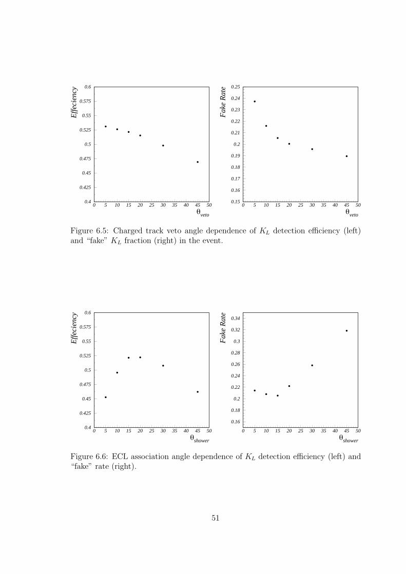
0.4
0.425
0.45
0.475
0.5
0.525
0.55
0.575
0.6
0 5 10 15 20 25 30 35 40 45 50
θveto
Eff
ecie
ncy
0.15
0.16
0.17
0.18
0.19
0.2
0.21
0.22
0.23
0.24
0.25
0 5 10 15 20 25 30 35 40 45 50
θveto
Fak
e R
ate
Figure 6.5: Charged track veto angle dependence of KL detection efficiency (left)and “fake” KL fraction (right) in the event.
0.4
0.425
0.45
0.475
0.5
0.525
0.55
0.575
0.6
0 5 10 15 20 25 30 35 40 45 50
θshower
Eff
ecie
ncy
0.16
0.18
0.2
0.22
0.24
0.26
0.28
0.3
0.32
0.34
0 5 10 15 20 25 30 35 40 45 50
θshower
Fak
e R
ate
Figure 6.6: ECL association angle dependence of KL detection efficiency (left) and“fake” rate (right).
51
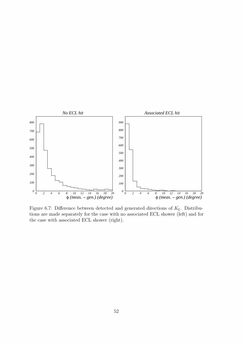
No ECL hit
0
100
200
300
400
500
600
700
800
0 2 4 6 8 10 12 14 16 18 20
φ (meas. − gen.) (degree)
Associated ECL hit
0
100
200
300
400
500
600
700
800
900
0 2 4 6 8 10 12 14 16 18 20
φ (meas. − gen.) (degree)
Figure 6.7: Difference between detected and generated directions of KL. Distribu-tions are made separately for the case with no associated ECL shower (left) and forthe case with associated ECL shower (right).
52
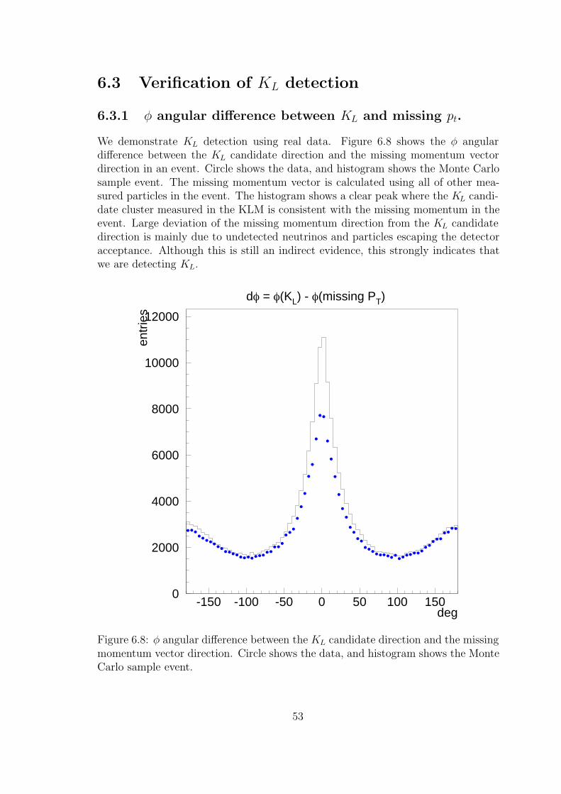
6.3 Verification of KL detection
6.3.1 φ angular difference between KL and missing pt.
We demonstrate KL detection using real data. Figure 6.8 shows the φ angulardifference between the KL candidate direction and the missing momentum vectordirection in an event. Circle shows the data, and histogram shows the Monte Carlosample event. The missing momentum vector is calculated using all of other mea-sured particles in the event. The histogram shows a clear peak where the KL candi-date cluster measured in the KLM is consistent with the missing momentum in theevent. Large deviation of the missing momentum direction from the KL candidatedirection is mainly due to undetected neutrinos and particles escaping the detectoracceptance. Although this is still an indirect evidence, this strongly indicates thatwe are detecting KL.
dφ = φ(KL) - φ(missing PT)
0
2000
4000
6000
8000
10000
12000
-150 -100 -50 0 50 100 150deg
entr
ies
Figure 6.8: φ angular difference between the KL candidate direction and the missingmomentum vector direction. Circle shows the data, and histogram shows the MonteCarlo sample event.
53
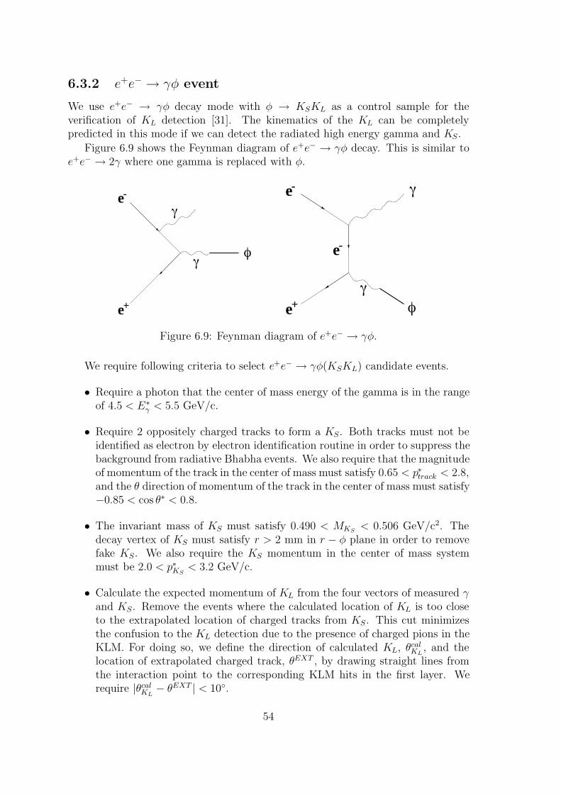
6.3.2 e+e− → γφ event
We use e+e− → γφ decay mode with φ → KSKL as a control sample for theverification of KL detection [31]. The kinematics of the KL can be completelypredicted in this mode if we can detect the radiated high energy gamma and KS.
Figure 6.9 shows the Feynman diagram of e+e− → γφ decay. This is similar toe+e− → 2γ where one gamma is replaced with φ.
-
e+
e
γ
γ
φ
+
e-
e-
e φγ
γ
Figure 6.9: Feynman diagram of e+e− → γφ.
We require following criteria to select e+e− → γφ(KSKL) candidate events.
• Require a photon that the center of mass energy of the gamma is in the rangeof 4.5 < E∗
γ < 5.5 GeV/c.
• Require 2 oppositely charged tracks to form a KS. Both tracks must not beidentified as electron by electron identification routine in order to suppress thebackground from radiative Bhabha events. We also require that the magnitudeof momentum of the track in the center of mass must satisfy 0.65 < p∗track < 2.8,and the θ direction of momentum of the track in the center of mass must satisfy−0.85 < cos θ∗ < 0.8.
• The invariant mass of KS must satisfy 0.490 < MKS< 0.506 GeV/c2. The
decay vertex of KS must satisfy r > 2 mm in r − φ plane in order to removefake KS. We also require the KS momentum in the center of mass systemmust be 2.0 < p∗KS
< 3.2 GeV/c.
• Calculate the expected momentum of KL from the four vectors of measured γand KS. Remove the events where the calculated location of KL is too closeto the extrapolated location of charged tracks from KS. This cut minimizesthe confusion to the KL detection due to the presence of charged pions in theKLM. For doing so, we define the direction of calculated KL, θcalKL
, and thelocation of extrapolated charged track, θEXT , by drawing straight lines fromthe interaction point to the corresponding KLM hits in the first layer. Werequire |θcalKL
− θEXT | < 10.
54

• We look for KL clusters in the event. If more than one KL cluster are found,we keep the one closest to θcalKL
.
• If the detected KL cluster is inside the 10 cone around the direction of calcu-lated KL, we declare that a KL is detected.
From Monte Carlo study, the detection efficiency of e+e− → γφ(KSKL) event isestimated to be 6.2%.
The triggered efficiency of e+e− → γφ event are estimated to be about 60% withthe Belle trigger scheme from Monte Carlo study. Most of the untriggered eventsare discarded by present Belle trigger scheme which suppresses Bhabha events, sincemost of e+e− → γφ events are also triggered with Bhabha event trigger conditionwhich looks simply energy sum of ECL.
The integrated luminosity used for this analysis is 1.2 fb−1. The total numberdetected as e+e− → γφ(KSKL) event is 95. Among these events, 25 KL events aredetected along the expected direction.
Figure 6.10 shows the KL detection efficiency as a function of momentum mea-sured by e+e− → γφ with data and Monte Carlo sample. Although statistics is stillsmall, one can see the large discrepancy between the data and Monte Carlo expec-tation. One of the cause of this discrepancy might be due to the contamination inselected KS. We need further study for this analysis.
6.4 KLM response in data and Monte Carlo
We studied the probability to make KLM clusters for KL, pion and kaon, usingMonte Carlo samples and data [33].
6.4.1 KLM cluster classification
Table 6.1 shows the average number of KLM clusters per hadronic event in the dataand Monte Carlo. The KLM clusters are divided into three categories : those passedthe KL selection criteria, those associated with charged track, and others. Threedifferent Monte Carlo samples, all hadronic events, BB enriched sample (R2 < 0.2),and continuum enriched (0.2 < R2 < 0.8), are used in this comparison. Except forthose classified as others, which are mostly one-hit clusters and presumably causedby noise hits, number of clusters in the data is lower compared with the MonteCarlo.
Table 6.2 shows a fraction of KL candidate which are associated with ECL. Herewe also observe a discrepancy between the data and Monte Carlo. This might bedue to beam-background in the ECL, which is not taken into account in the MonteCarlo in this study.
An average number of KL per event in the data comes out to be 0.35, whereasMonte Carlo prediction is 0.47. Fraction of detected KL in the data is 40% by theKLM only, and 60% by a combination of KLM and ECL. Monte Carlo predict thesefractions are about 50% and 50%.
55
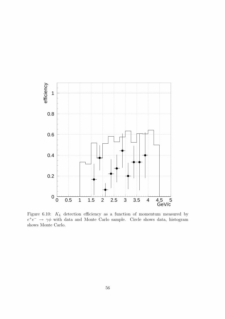
0
0.2
0.4
0.6
0.8
1
0 0.5 1 1.5 2 2.5 3 3.5 4 4.5 5GeV/c
effic
ienc
y
Figure 6.10: KL detection efficiency as a function of momentum measured bye+e− → γφ with data and Monte Carlo sample. Circle shows data, histogramshows Monte Carlo.
56
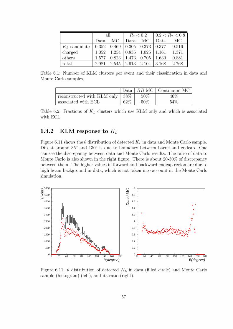
all R2 < 0.2 0.2 < R2 < 0.8Data MC Data MC Data MC
KL candidate 0.352 0.469 0.305 0.373 0.377 0.516charged 1.052 1.254 0.835 1.025 1.161 1.371others 1.577 0.823 1.473 0.705 1.630 0.881total 2.981 2.545 2.613 2.104 3.168 2.768
Table 6.1: Number of KLM clusters per event and their classification in data andMonte Carlo samples.
Data BB MC Continuum MCreconstructed with KLM only 38% 50% 46%associated with ECL 62% 50% 54%
Table 6.2: Fractions of KL clusters which use KLM only and which is associatedwith ECL.
6.4.2 KLM response to KL
Figure 6.11 shows the θ distribution of detected KL in data and Monte Carlo sample.Dip at around 35 and 130 is due to boundary between barrel and endcap. Onecan see the discrepancy between data and Monte Carlo results. The ratio of data toMonte Carlo is also shown in the right figure. There is about 20-30% of discrepancybetween them. The higher values in forward and backward endcap region are due tohigh beam background in data, which is not taken into account in the Monte Carlosimulation.
0
500
1000
1500
2000
2500
3000
3500
4000
4500
5000
0 20 40 60 80 100 120 140 160 180
θ(degree)
Eve
nts
0
0.2
0.4
0.6
0.8
1
1.2
1.4
1.6
1.8
2
0 20 40 60 80 100 120 140 160 180
θ(degree)
Dat
a / M
C
Figure 6.11: θ distribution of detected KL in data (filled circle) and Monte Carlosample (histogram) (left), and its ratio (right).
57

6.4.3 KLM response to π± and K±
The pions and kaons are identified by theK/π separation routine. Matching betweenKLM clusters and pion or kaon tracks are done by the KL identification methodwritten in section 6.1.
Figure 6.12 shows the θ and φ distribution of the fraction to make KLM clustersfor pions of momentum between 0.8 and 1.2 GeV/c. Monte Carlo results and realdata are shown in the figure. One can see the discrepancy between them, showingthat Monte Carlo is always higher than data.
Figure 6.13 shows the fraction of pions making KLM clusters as a function ofmomentum. Filled circle is for Monte Carlo and open square is for data. The ratioof data to the Monte Carlo are also shown in order to quantify the discrepancy.
The same study was carried out for kaon. Figure 6.14 shows the θ and φ distri-bution of the fraction of making KLM clusters for kaons of momentum between 0.8and 1.2 GeV/c.
Figure 6.15 shows the fraction of kaons making KLM clusters as a function ofmomentum. The ratio of data to the Monte Carlo are also shown in order to quantifythe discrepancy.
6.4.4 Summary of KLM response to KL, π± and K±
There is about 20-30% discrepancy between data and Monte Carlo in the KLMresponse to either KL, pions or kaons. We have noticed that the hadron-showermodel which is used in the Monte Carlo might not be representing the real datacorrectly. The study to modify the hadron-shower model in full detector simulatorhas been started, so we will get better agreement when the study completes.
58
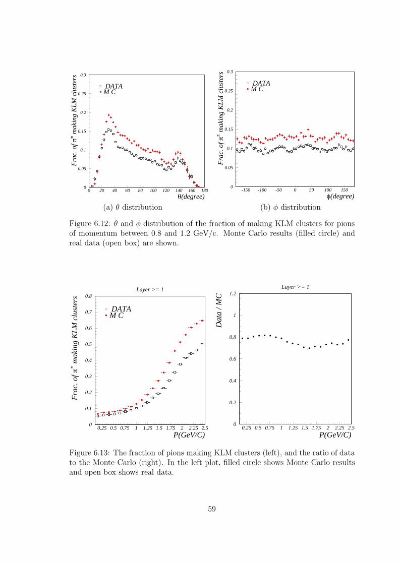
0
0.05
0.1
0.15
0.2
0.25
0.3
0 20 40 60 80 100 120 140 160 180
θ(degree)
Fra
c. o
f π± m
akin
g K
LM
clu
ster
s
DATAM C
0
0.05
0.1
0.15
0.2
0.25
0.3
-150 -100 -50 0 50 100 150
φ(degree)
Fra
c. o
f π± m
akin
g K
LM
clu
ster
s
DATAM C
(a) θ distribution (b) φ distribution
Figure 6.12: θ and φ distribution of the fraction of making KLM clusters for pionsof momentum between 0.8 and 1.2 GeV/c. Monte Carlo results (filled circle) andreal data (open box) are shown.
Layer >= 1
0
0.1
0.2
0.3
0.4
0.5
0.6
0.7
0.8
0.25 0.5 0.75 1 1.25 1.5 1.75 2 2.25 2.5
P(GeV/C)
Fra
c. o
f π± m
akin
g K
LM
clu
ster
s
DATAM C
Layer >= 1
0
0.2
0.4
0.6
0.8
1
1.2
0.25 0.5 0.75 1 1.25 1.5 1.75 2 2.25 2.5
P(GeV/C)
Dat
a / M
C
Figure 6.13: The fraction of pions making KLM clusters (left), and the ratio of datato the Monte Carlo (right). In the left plot, filled circle shows Monte Carlo resultsand open box shows real data.
59
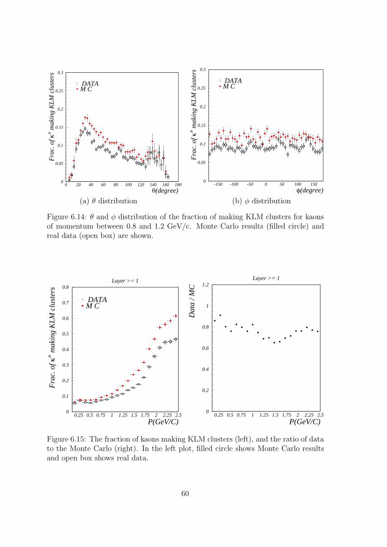
0
0.05
0.1
0.15
0.2
0.25
0.3
0 20 40 60 80 100 120 140 160 180
θ(degree)
Fra
c. o
f κ± m
akin
g K
LM
clu
ster
s
DATAM C
0
0.05
0.1
0.15
0.2
0.25
0.3
-150 -100 -50 0 50 100 150
φ(degree)F
rac.
of κ
± mak
ing
KL
M c
lust
ers
DATAM C
(a) θ distribution (b) φ distribution
Figure 6.14: θ and φ distribution of the fraction of making KLM clusters for kaonsof momentum between 0.8 and 1.2 GeV/c. Monte Carlo results (filled circle) andreal data (open box) are shown.
Layer >= 1
0
0.1
0.2
0.3
0.4
0.5
0.6
0.7
0.8
0.25 0.5 0.75 1 1.25 1.5 1.75 2 2.25 2.5
P(GeV/C)
Fra
c. o
f κ± m
akin
g K
LM
clu
ster
s
DATAM C
Layer >= 1
0
0.2
0.4
0.6
0.8
1
1.2
0.25 0.5 0.75 1 1.25 1.5 1.75 2 2.25 2.5
P(GeV/C)
Dat
a / M
C
Figure 6.15: The fraction of kaons making KLM clusters (left), and the ratio of datato the Monte Carlo (right). In the left plot, filled circle shows Monte Carlo resultsand open box shows real data.
60
Chapter 7
Reconstruction of B0 → J/ψ +KLdecays
In this chapter we describe the reconstruction procedure of B0 → J/ψ +KL event.Signal yield and background estimation are also described.
7.1 Data set and Monte Carlo events
Data set used in this analysis is 6.2 fb−1 that was taken during the run period fromJune 1999 to July 2000. As Monte Carlo sample, we use 600,000 inclusive J/ψevents. This corresponds to 223 fb−1 data of Υ(4S) decays. They are generated asΥ(4S) → BB with the B0B0 mixing being turned off. We allow B0 to decay onlyto J/ψX and B0 to decay generically. The J/ψ is allowed to decay into e+e− andµ+µ− each with 50% probability.
For the study of J/ψKL signal events and particular background mode such asJ/ψK∗0(KLπ
0), we use the generator information for those 600,000 inclusive J/ψevents.
7.2 Hadronic event selection
The hadronic events were selected by following criteria.
• At least three “good” tracks were coming from the interaction point, where
“good” track was defined by (i) |r| < 2.0 cm and |z| < 4.0 cm at the closest
approach at the beam axis, (ii) momentum projected onto the xy−plane > 0.1
GeV/c .
• More than one “good” cluster must be observed in the barrel region of the
calorimeter, where “good” cluster was defined in such a way that it was de-
tected in the good acceptance region with an energy deposit greater than 0.1
GeV, where no track were associated with the cluster.
61
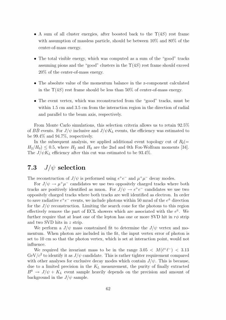
• A sum of all cluster energies, after boosted back to the Υ(4S) rest frame
with assumption of massless particle, should be between 10% and 80% of the
center-of-mass energy.
• The total visible energy, which was computed as a sum of the “good” tracks
assuming pions and the “good” clusters in the Υ(4S) rest frame should exceed
20% of the center-of-mass energy.
• The absolute value of the momentum balance in the z-component calculated
in the Υ(4S) rest frame should be less than 50% of center-of-mass energy.
• The event vertex, which was reconstructed from the “good” tracks, must be
within 1.5 cm and 3.5 cm from the interaction region in the direction of radial
and parallel to the beam axis, respectively.
From Monte Carlo simulations, this selection criteria allows us to retain 92.5%of BB events. For J/ψ inclusive and J/ψKL events, the efficiency was estimated tobe 99.4% and 94.7%, respectively.
In the subsequent analysis, we applied additional event topology cut of R2(=H2/H0) ≤ 0.5, where H2 and H0 are the 2nd and 0th Fox-Wolfram moments [34].The J/ψKL efficiency after this cut was estimated to be 93.4%.
7.3 J/ψ selection
The reconstruction of J/ψ is performed using e+e− and µ+µ− decay modes.For J/ψ → µ+µ− candidates we use two oppositely charged tracks where both
tracks are positively identified as muon. For J/ψ → e+e− candidates we use twooppositely charged tracks where both tracks are well identified as electron. In orderto save radiative e+e− events, we include photons within 50 mrad of the e± directionfor the J/ψ reconstruction. Limiting the search cone for the photons to this regioneffectively remove the part of ECL showers which are associated with the e±. Wefurther require that at least one of the lepton has one or more SVD hit in rφ stripand two SVD hits in z strip.
We perform a J/ψ mass constrained fit to determine the J/ψ vertex and mo-mentum. When photon are included in the fit, the input vertex error of photon isset to 10 cm so that the photon vertex, which is set at interaction point, would notinfluence.
We required the invariant mass to be in the range 3.05 < M(+−) < 3.13GeV/c2 to identify it as J/ψ candidate. This is rather tighter requirement comparedwith other analyses for exclusive decay modes which contain J/ψ. This is because,due to a limited precision in the KL measurement, the purity of finally extractedB0 → J/ψ + KL event sample heavily depends on the precision and amount ofbackground in the J/ψ sample.
62
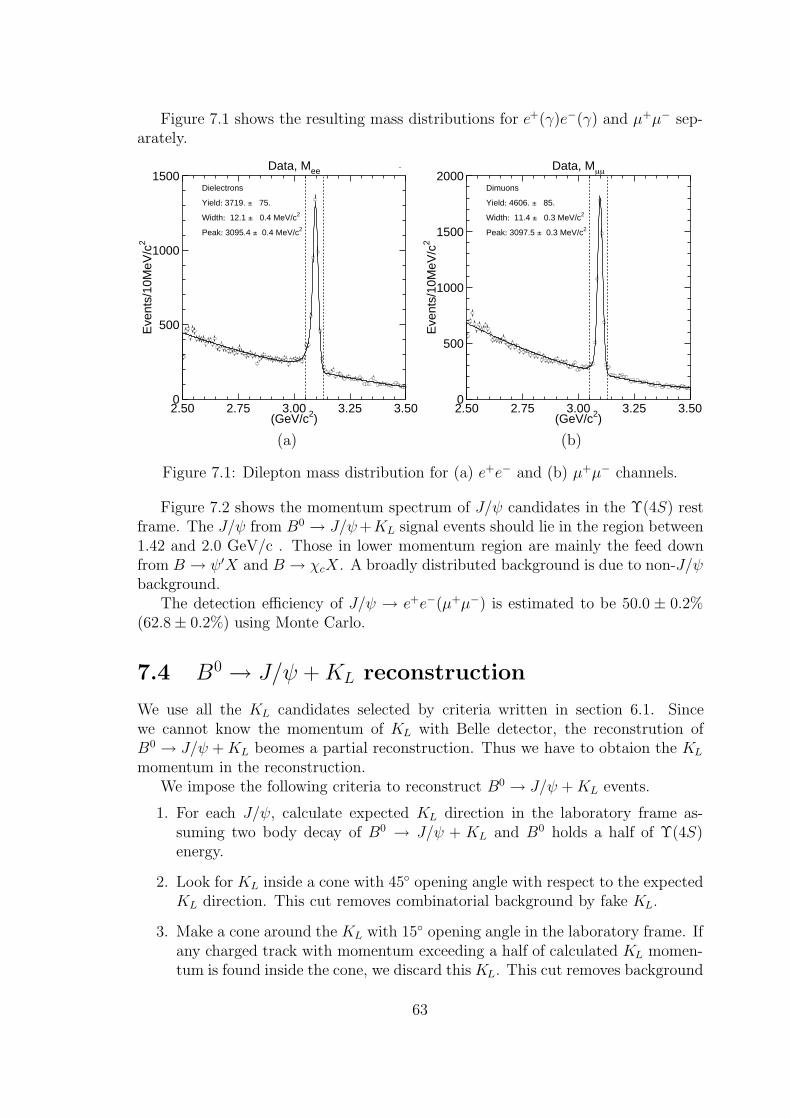
Figure 7.1 shows the resulting mass distributions for e+(γ)e−(γ) and µ+µ− sep-arately.
Data, Mee
2.50 2.75 3.00 3.25 3.50(GeV/c2)
0
500
1000
1500
Eve
nts/
10M
eV/c
2
Dielectrons
Yield: 3719. ± 75.
Width: 12.1 ± 0.4 MeV/c2
Peak: 3095.4 ± 0.4 MeV/c2
Data, Mµµ
2.50 2.75 3.00 3.25 3.50(GeV/c2)
0
500
1000
1500
2000
Eve
nts/
10M
eV/c
2
Dimuons
Yield: 4606. ± 85.
Width: 11.4 ± 0.3 MeV/c2
Peak: 3097.5 ± 0.3 MeV/c2
(a) (b)
Figure 7.1: Dilepton mass distribution for (a) e+e− and (b) µ+µ− channels.
Figure 7.2 shows the momentum spectrum of J/ψ candidates in the Υ(4S) restframe. The J/ψ from B0 → J/ψ+KL signal events should lie in the region between1.42 and 2.0 GeV/c . Those in lower momentum region are mainly the feed downfrom B → ψ′X and B → χcX. A broadly distributed background is due to non-J/ψbackground.
The detection efficiency of J/ψ → e+e−(µ+µ−) is estimated to be 50.0 ± 0.2%(62.8 ± 0.2%) using Monte Carlo.
7.4 B0 → J/ψ +KL reconstruction
We use all the KL candidates selected by criteria written in section 6.1. Sincewe cannot know the momentum of KL with Belle detector, the reconstrution ofB0 → J/ψ +KL beomes a partial reconstruction. Thus we have to obtaion the KL
momentum in the reconstruction.We impose the following criteria to reconstruct B0 → J/ψ +KL events.
1. For each J/ψ, calculate expected KL direction in the laboratory frame as-suming two body decay of B0 → J/ψ + KL and B0 holds a half of Υ(4S)energy.
2. Look for KL inside a cone with 45 opening angle with respect to the expectedKL direction. This cut removes combinatorial background by fake KL.
3. Make a cone around the KL with 15 opening angle in the laboratory frame. Ifany charged track with momentum exceeding a half of calculated KL momen-tum is found inside the cone, we discard this KL. This cut removes background
63
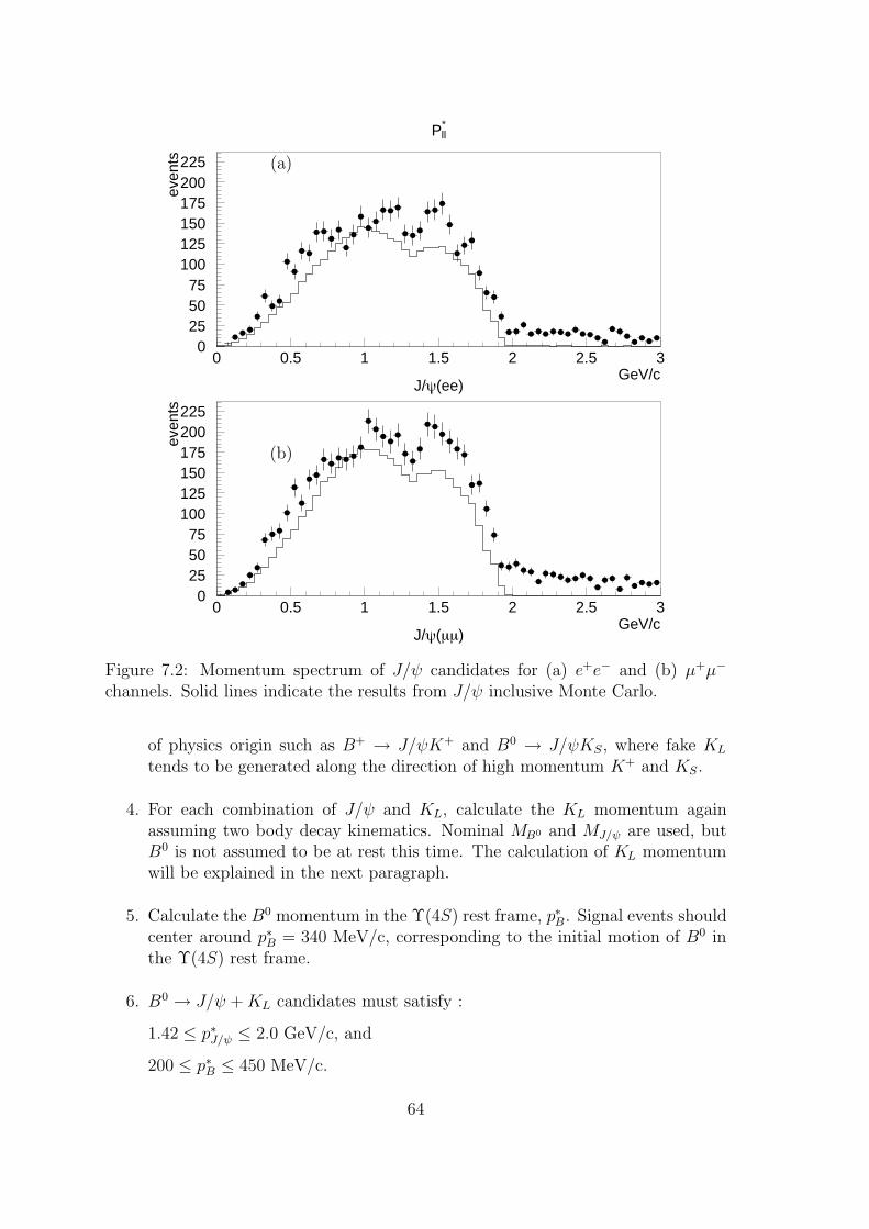
J/ψ(ee)
P*ll
0255075
100125150175200225
0 0.5 1 1.5 2 2.5 3GeV/c
even
ts
J/ψ(µµ)
0255075
100125150175200225
0 0.5 1 1.5 2 2.5 3GeV/c
even
ts(a)
(b)
Figure 7.2: Momentum spectrum of J/ψ candidates for (a) e+e− and (b) µ+µ−
channels. Solid lines indicate the results from J/ψ inclusive Monte Carlo.
of physics origin such as B+ → J/ψK+ and B0 → J/ψKS, where fake KL
tends to be generated along the direction of high momentum K+ and KS.
4. For each combination of J/ψ and KL, calculate the KL momentum againassuming two body decay kinematics. Nominal MB0 and MJ/ψ are used, butB0 is not assumed to be at rest this time. The calculation of KL momentumwill be explained in the next paragraph.
5. Calculate the B0 momentum in the Υ(4S) rest frame, p∗B. Signal events shouldcenter around p∗B = 340 MeV/c, corresponding to the initial motion of B0 inthe Υ(4S) rest frame.
6. B0 → J/ψ +KL candidates must satisfy :
1.42 ≤ p∗J/ψ ≤ 2.0 GeV/c, and
200 ≤ p∗B ≤ 450 MeV/c.
64
The KL momentum is obtained by following calculation. We know the directionof the KL momentum from the information of the ECL and the KLM by assumingthat the KL was generated at interaction point. The only unknown is the magnitudeofKL momentum, |pKL
|, when we assume two body decay kinematics. We can obtainit by solving the following equation.
m2B = (EJP + EKL
)2 −(pJ/ψ + pKL
)2
=(EJP +
√|pKL
|2 +m2KL
)2
−(|pJ/ψ|2 + |pKL
|2 + 2|pJ/ψ||pKL| cos θ
)2(7.1)
where
mB, mJ/ψ, mKL: invariant mass of B0, J/ψ, KL,
EJ/ψ, pJ/ψ : measured energy and momentum of J/ψ,
pKL: momentum of KL to be solved,
θ : opening angle between pJ/ψ and pKL.
All the parameters are the value in the laboratory frame. This is the second orderequation for |pKL
|. The solution is expressed as
pKL =a · b + EJ/ψ
√a2 − 4m2
KL(E2
J/ψ − b2)
2(E2J/ψ − b2)
. (7.2)
a ≡ m2B −m2
J/ψ −m2KL,
b ≡ |pJ/ψ| cos θ.
The problem of this method is that this is not a fit but only a calculation, so wecannot evaluate the error of |pKL
|.Figure 7.3 shows the spectrum of calculated KL momentum in the Υ(4S) rest
frame. The KL from B0 → J/ψ+KL signal events should lie between 1.55 and 1.85GeV/c as shown with broken line in the figure. Those from B → J/ψKLπ back-ground should lie between 1.6 and 1.9 GeV/c. A long tail toward higher momentumregion is due to low momentum J/ψ which come from the feed down.
Figure 7.4 shows scatter plots of p∗J/ψ versus p∗B for data and different sourcesin Monte Carlo. According to the Monte Carlo, about 88% of the signal eventsis contained in the region of 200 ≤ p∗B ≤ 450 MeV/c . The background fromB → J/ψKLπ also peaks near the signal region although the mean is shifted byabout 80 MeV/c toward higher p∗B and the width is much broader. Here the J/ψKLπbackground is a sum of both resonant case (J/ψK∗) and non-resonant case, andcontributions from B± → J/ψKLπ
± and B0 → J/ψKLπ0 are summed. According
to the Monte Carlo, about a half of these events remains in the signal p∗B region. Forneither of the two cases, hardly any events populate outside of the 1.42 ≤ p∗J/ψ ≤ 2.0GeV/c region.
65
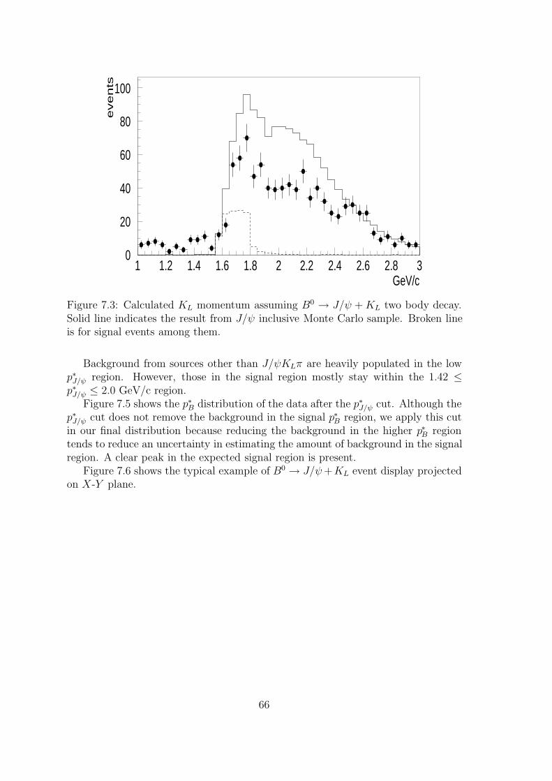
0
20
40
60
80
100
1 1.2 1.4 1.6 1.8 2 2.2 2.4 2.6 2.8 3GeV/c
eve
nts
Figure 7.3: Calculated KL momentum assuming B0 → J/ψ +KL two body decay.Solid line indicates the result from J/ψ inclusive Monte Carlo sample. Broken lineis for signal events among them.
Background from sources other than J/ψKLπ are heavily populated in the lowp∗J/ψ region. However, those in the signal region mostly stay within the 1.42 ≤p∗J/ψ ≤ 2.0 GeV/c region.
Figure 7.5 shows the p∗B distribution of the data after the p∗J/ψ cut. Although thep∗J/ψ cut does not remove the background in the signal p∗B region, we apply this cutin our final distribution because reducing the background in the higher p∗B regiontends to reduce an uncertainty in estimating the amount of background in the signalregion. A clear peak in the expected signal region is present.
Figure 7.6 shows the typical example of B0 → J/ψ+KL event display projectedon X-Y plane.
66
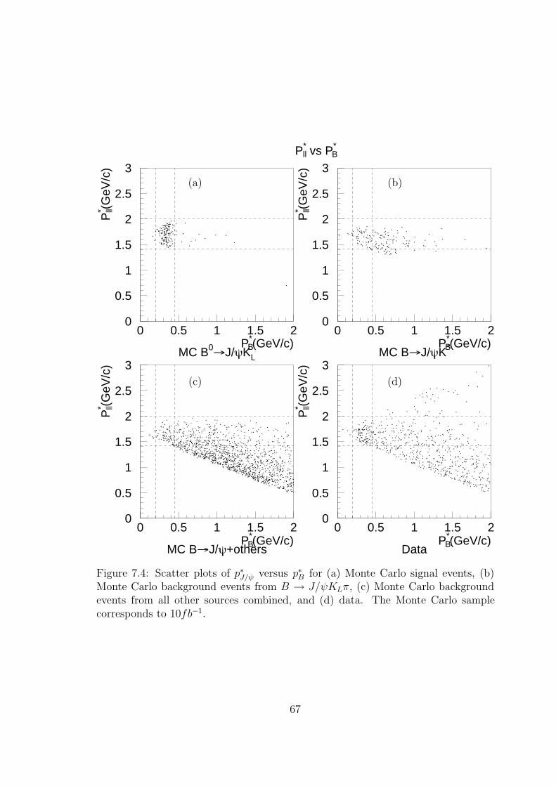
P*ll vs P*
B
0
0.5
1
1.5
2
2.5
3
0 0.5 1 1.5 2
MC B0→J/ψKL
P*B(GeV/c)
P* ll(
GeV
/c)
0
0.5
1
1.5
2
2.5
3
0 0.5 1 1.5 2
MC B→J/ψK*P*B(GeV/c)
P* ll(
GeV
/c)
0
0.5
1
1.5
2
2.5
3
0 0.5 1 1.5 2
MC B→J/ψ+othersP*
B(GeV/c)
P* ll(
GeV
/c)
0
0.5
1
1.5
2
2.5
3
0 0.5 1 1.5 2
DataP*
B(GeV/c)
P* ll(
GeV
/c)
(a) (b)
(c) (d)
Figure 7.4: Scatter plots of p∗J/ψ versus p∗B for (a) Monte Carlo signal events, (b)Monte Carlo background events from B → J/ψKLπ, (c) Monte Carlo backgroundevents from all other sources combined, and (d) data. The Monte Carlo samplecorresponds to 10fb−1.
67
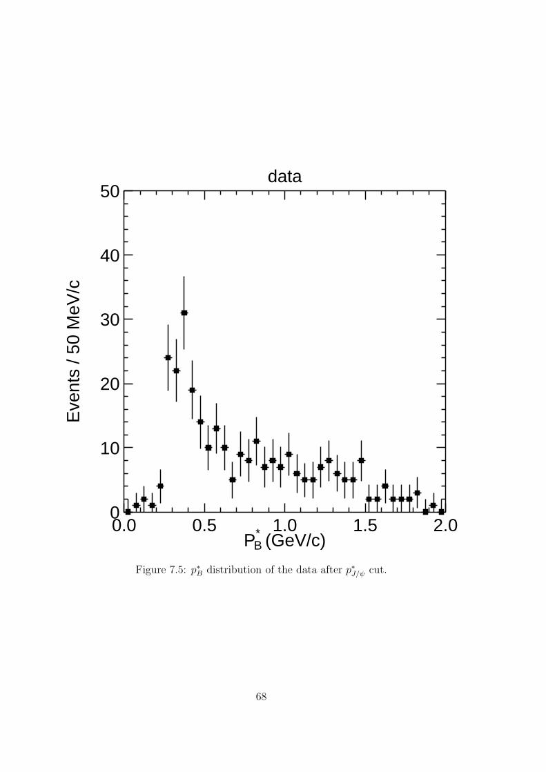
data
0.0 0.5 1.0 1.5 2.0P*
B (GeV/c)
0
10
20
30
40
50
Eve
nts
/ 50
MeV
/c
Figure 7.5: p∗B distribution of the data after p∗J/ψ cut.
68
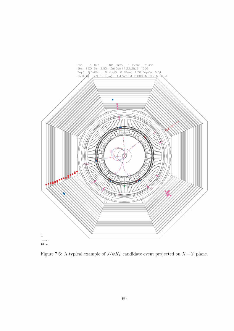
20 cm
Figure 7.6: A typical example of J/ψKL candidate event projected on X−Y plane.
69
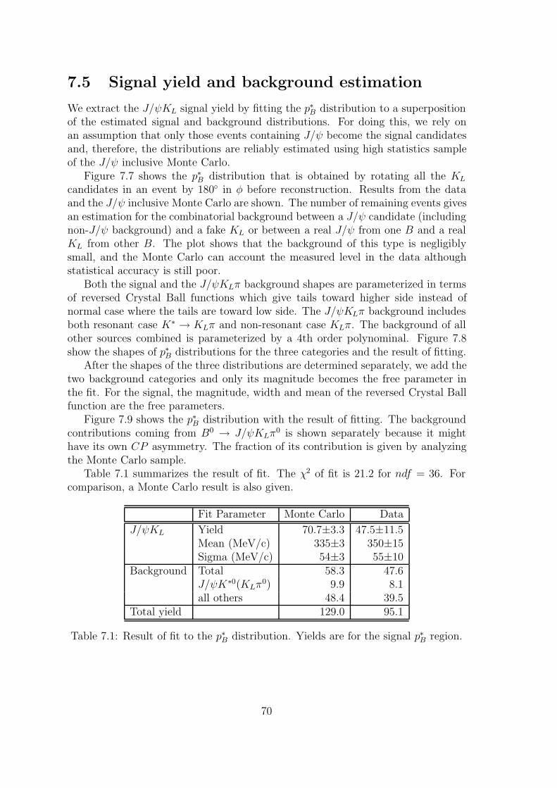
7.5 Signal yield and background estimation
We extract the J/ψKL signal yield by fitting the p∗B distribution to a superpositionof the estimated signal and background distributions. For doing this, we rely onan assumption that only those events containing J/ψ become the signal candidatesand, therefore, the distributions are reliably estimated using high statistics sampleof the J/ψ inclusive Monte Carlo.
Figure 7.7 shows the p∗B distribution that is obtained by rotating all the KL
candidates in an event by 180 in φ before reconstruction. Results from the dataand the J/ψ inclusive Monte Carlo are shown. The number of remaining events givesan estimation for the combinatorial background between a J/ψ candidate (includingnon-J/ψ background) and a fake KL or between a real J/ψ from one B and a realKL from other B. The plot shows that the background of this type is negligiblysmall, and the Monte Carlo can account the measured level in the data althoughstatistical accuracy is still poor.
Both the signal and the J/ψKLπ background shapes are parameterized in termsof reversed Crystal Ball functions which give tails toward higher side instead ofnormal case where the tails are toward low side. The J/ψKLπ background includesboth resonant case K∗ → KLπ and non-resonant case KLπ. The background of allother sources combined is parameterized by a 4th order polynominal. Figure 7.8show the shapes of p∗B distributions for the three categories and the result of fitting.
After the shapes of the three distributions are determined separately, we add thetwo background categories and only its magnitude becomes the free parameter inthe fit. For the signal, the magnitude, width and mean of the reversed Crystal Ballfunction are the free parameters.
Figure 7.9 shows the p∗B distribution with the result of fitting. The backgroundcontributions coming from B0 → J/ψKLπ
0 is shown separately because it mighthave its own CP asymmetry. The fraction of its contribution is given by analyzingthe Monte Carlo sample.
Table 7.1 summarizes the result of fit. The χ2 of fit is 21.2 for ndf = 36. Forcomparison, a Monte Carlo result is also given.
Fit Parameter Monte Carlo Data
J/ψKL Yield 70.7±3.3 47.5±11.5Mean (MeV/c) 335±3 350±15Sigma (MeV/c) 54±3 55±10
Background Total 58.3 47.6J/ψK∗0(KLπ
0) 9.9 8.1all others 48.4 39.5
Total yield 129.0 95.1
Table 7.1: Result of fit to the p∗B distribution. Yields are for the signal p∗B region.
70
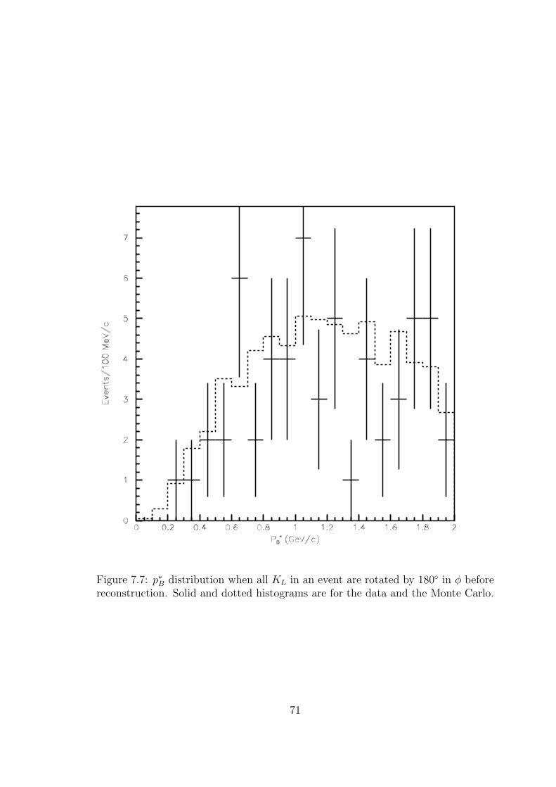
Figure 7.7: p∗B distribution when all KL in an event are rotated by 180 in φ beforereconstruction. Solid and dotted histograms are for the data and the Monte Carlo.
71
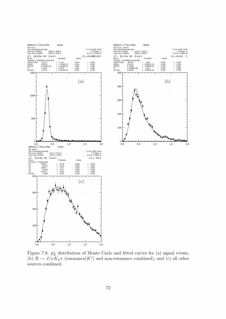
0.0 0.5 1.0 1.5 2.00
500
1000
1500
MINUIT χ2 Fit to Plot 31&0MC J/ψ KLFile: Generated internally 17-JUL-2000 19:48Plot Area Total/Fit 3839.0 / 3839.0Func Area Total/Fit 3754.4 / 3754.4
Fit Status 3E.D.M. 2.226E-06
χ2= 84.9 for 40 - 5 d.o.f., C.L.=0.498E-03%Errors Parabolic MinosFunction 1: Modified Crystal BallAMPLITUDE 1131.5 ± 27.16 - 0.000 + 0.000MEAN 0.33312 ± 1.1033E-03 - 0.000 + 0.000WIDTH 5.97281E-02 ± 1.1090E-03 - 0.000 + 0.000N 1.3975 ± 0.1013 - 0.000 + 0.000ALPHA 1.6716 ± 6.2518E-02 - 0.000 + 0.000
0.0 0.5 1.0 1.5 2.00
100
200
300
400
500
MINUIT χ2 Fit to Plot 35&0MC J/ψ KL π (sum)File: Generated internally 17-JUL-2000 19:48Plot Area Total/Fit 4152.0 / 4152.0Func Area Total/Fit 4094.5 / 4094.5
Fit Status 3E.D.M. 7.560E-06
χ2= 62.2 for 40 - 5 d.o.f., C.L.=0.314 %Errors Parabolic MinosFunction 2: Modified Crystal BallAMPLITUDE 382.83 ± 1.394 - 0.000 + 0.000MEAN 0.41161 ± 6.8857E-03 - 0.000 + 0.000WIDTH 0.13932 ± 4.0894E-03 - 0.000 + 0.000N 1.19059E+06 ± 1.414 - 0.000 + 0.000ALPHA 0.41538 ± 1.8907E-02 - 0.000 + 0.000
0.0 0.5 1.0 1.5 2.00
100
200
300
400
MINUIT χ2 Fit to Plot 37&0MC othersFile: Generated internally 17-JUL-2000 19:48Plot Area Total/Fit 7412.0 / 7412.0Func Area Total/Fit 7357.0 / 7357.0
Fit Status 3E.D.M. 2.185E-16
χ2= 51.6 for 40 - 5 d.o.f., C.L.= 3.5%Errors Parabolic MinosFunction 3: PolynominalA0 -199.54 ± 12.49 - 0.000 + 0.000A1 2079.1 ± 92.43 - 0.000 + 0.000A2 -2687.6 ± 175.2 - 0.000 + 0.000A3 1293.5 ± 122.1 - 0.000 + 0.000A4 -220.10 ± 28.34 - 0.000 + 0.000SCALE∗ 1.0000 ± 0.000 - 0.000 + 0.000
(a) (b)
(c)
Figure 7.8: p∗B distribution of Monte Carlo and fitted curves for (a) signal events,(b) B → J/ψKLπ (resonance(K∗) and non-resonance combined), and (c) all othersources combined.
72
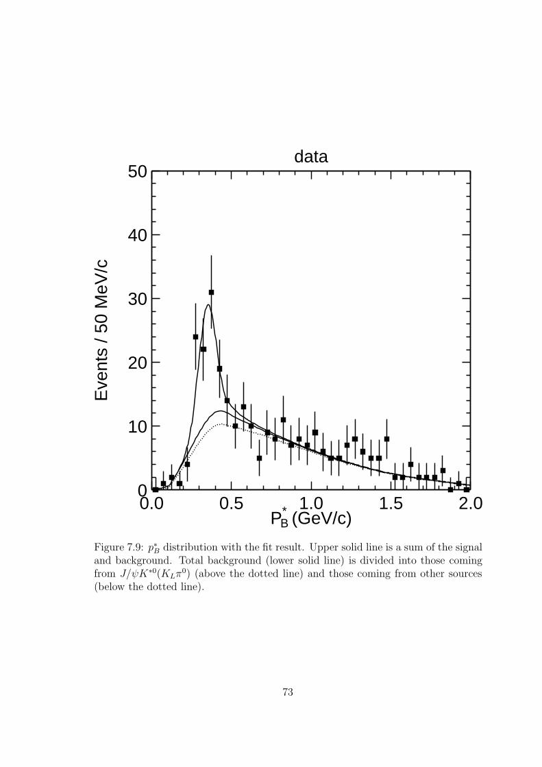
data
0.0 0.5 1.0 1.5 2.0P*
B (GeV/c)
0
10
20
30
40
50
Eve
nts
/ 50
MeV
/c
Figure 7.9: p∗B distribution with the fit result. Upper solid line is a sum of the signaland background. Total background (lower solid line) is divided into those comingfrom J/ψK∗0(KLπ
0) (above the dotted line) and those coming from other sources(below the dotted line).
73
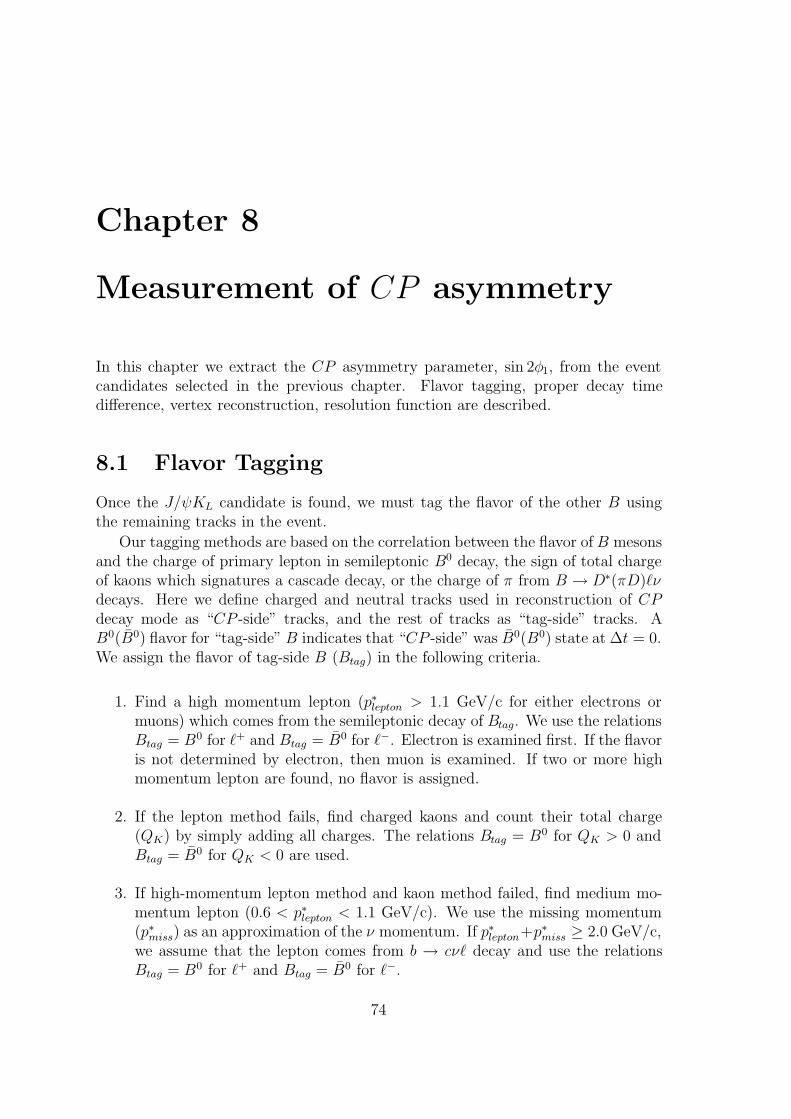
Chapter 8
Measurement of CP asymmetry
In this chapter we extract the CP asymmetry parameter, sin 2φ1, from the eventcandidates selected in the previous chapter. Flavor tagging, proper decay timedifference, vertex reconstruction, resolution function are described.
8.1 Flavor Tagging
Once the J/ψKL candidate is found, we must tag the flavor of the other B usingthe remaining tracks in the event.
Our tagging methods are based on the correlation between the flavor of B mesonsand the charge of primary lepton in semileptonic B0 decay, the sign of total chargeof kaons which signatures a cascade decay, or the charge of π from B → D∗(πD)νdecays. Here we define charged and neutral tracks used in reconstruction of CPdecay mode as “CP -side” tracks, and the rest of tracks as “tag-side” tracks. AB0(B0) flavor for “tag-side” B indicates that “CP -side” was B0(B0) state at ∆t = 0.We assign the flavor of tag-side B (Btag) in the following criteria.
1. Find a high momentum lepton (p∗lepton > 1.1 GeV/c for either electrons ormuons) which comes from the semileptonic decay of Btag. We use the relationsBtag = B0 for + and Btag = B0 for −. Electron is examined first. If the flavoris not determined by electron, then muon is examined. If two or more highmomentum lepton are found, no flavor is assigned.
2. If the lepton method fails, find charged kaons and count their total charge(QK) by simply adding all charges. The relations Btag = B0 for QK > 0 andBtag = B0 for QK < 0 are used.
3. If high-momentum lepton method and kaon method failed, find medium mo-mentum lepton (0.6 < p∗lepton < 1.1 GeV/c). We use the missing momentum(p∗miss) as an approximation of the ν momentum. If p∗lepton+p∗miss ≥ 2.0 GeV/c,we assume that the lepton comes from b → cν decay and use the relationsBtag = B0 for + and Btag = B0 for −.
74
_b
_s
ν
l+
c_
BK
+0
d
D*-
π-
slow
W+
Figure 8.1: Illustration for the flavor tagging method.
4. If above method failed, find low momentum (p∗ < 200 MeV/c) charged trackconsistent with a π from the D∗ → Dπ decay. We use the relations Btag = B0
for π− and Btag = B0 for π+.
Figure 8.1 illustrates the schematics of our flavor tagging method.The efficiency and wrong tag fraction is obtained using exclusively reconstructed
B → D(∗)ν events which are self tagging decay modes, and the full Monte Carlosimulation. Here, we define
• Tagging efficiency: εtag = Ntag/Nrec, where Ntag and Nrec are number of taggedand reconstructed CP events, respectively.
• Wrong-tag fraction: ω =(number of wrongly tagged events)/ (total number oftagged events)
Taking into account the wrong-tag fraction, the time evolution of the oppositeflavor (OF) and same flavor (SF) neutral B meson pair is given as
POF ∝ 1 + (1 − 2ω) cos(∆md∆t), (8.1)
PSF ∝ 1 + (1 − 2ω) cos(∆md∆t). (8.2)
The wrong-tag fraction determines the oscillation amplitude of the OF-SF asymme-try.
Amix =OF − SF
OF + SF= (1 − 2ω) cos(∆md∆t) (8.3)
We fit the time evolution of the OF and SF events simultaneously and obtain thewrong-tag fraction [35].
We use the following decay modes:
• B0 → D∗−+ν,D∗− → D0π−
– D0 → K+π−
75
– D0 → K+π−π0
– D0 → K+π+π−π−
• B0 → D−+ν,D− → K+π−π−
The vertex position of D(∗)ν is obtained in the following way. First, we fit theD vertex using K and π tracks, where K and π mass is constrained to the worldaverage D mass. For the Kππ0 mode, D mass constraint is turned off. Then, weperform a vertex fitting of and D tracks to obtain the B vertex. The slow piontrack from D∗ is not used in the fit, since it does not help to improve B vertexresolution.
We apply the flavor tagging mentioned above to the tag-side, treating the tracksused by the reconstruction of D(∗)ν decay as the CP -side tracks. We also use thesame method to obtain a tag-side vertex position as this analysis, which is describedin detail later.
We obtain the wrong-tag fraction together with the mixing parameter ∆md byfitting the ∆z distribution of the SF and OF events.
The results are
ωlepton = 0.071 ± 0.045 and ωK = 0.199 ± 0.070. (8.4)
The tagging efficiencies are obtained using the same D(∗)ν samples.
εlepton = 0.142 ± 0.021, (8.5)
εK = 0.279 ± 0.042. (8.6)
We have also checked the wrong-tag fraction using the time-integrated numberof OF and SF events with D(∗)∓±ν sample. Taking into account the B0
d-B0d mixing
effect, ω is obtained by
ω =χobs − χd1 − 2χd
, χd =τ 2B0∆m2
2(1 + τ 2B0∆m2)
(8.7)
where χobs = NSF/(NOF +NSF ), and we use χd = 0.172 ± 0.010 [13]. Both resultsare consistent within errors.
The tagging efficiencies and wrong tag fractions of mid-momentum lepton andslow pion are obtained from Monte Carlo analysis. The efficiencies for mid-momentumlepton and slow pion are 3% and 7%, and wrong tag fractions are 29% and 34%,respectively.
The results are summarized in table 8.1, These give total efficiency of 0.52, andthe total effective tagging efficiency (εeff ), defined as a sum of ε(1 − 2ω) over alltagging methods, is 0.218.
We find a total of 42 tagged events, of which 8 events were tagged by a high-momentum e, 7 events by a high-momentum µ, 19 events by K±, 0 events bymedium-momentum e, 2 events by medium-momentum µ, and 6 events by slow π.
76
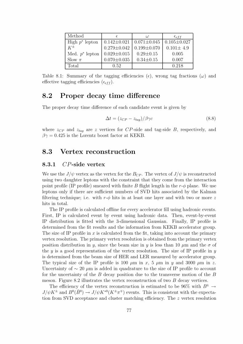
Method ε ω εeffHigh p∗ lepton 0.142±0.021 0.071±0.045 0.105±0.027K± 0.279±0.042 0.199±0.070 0.101± 4.9Med. p∗ lepton 0.029±0.015 0.29±0.15 0.005Slow π 0.070±0.035 0.34±0.15 0.007Total 0.52 0.218
Table 8.1: Summary of the tagging efficiencies (ε), wrong tag fractions (ω) andeffective tagging efficiencies (εeff ).
8.2 Proper decay time difference
The proper decay time difference of each candidate event is given by
∆t = (zCP − ztag)/βγc (8.8)
where zCP and ztag are z vertices for CP -side and tag-side B, respectively, andβγ = 0.425 is the Lorentz boost factor at KEKB.
8.3 Vertex reconstruction
8.3.1 CP -side vertex
We use the J/ψ vertex as the vertex for the BCP . The vertex of J/ψ is reconstructedusing two daughter leptons with the constraint that they come from the interactionpoint profile (IP profile) smeared with finite B flight length in the r-φ plane. We useleptons only if there are sufficient numbers of SVD hits associated by the Kalmanfiltering technique; i.e. with r-φ hits in at least one layer and with two or more zhits in total.
The IP profile is calculated offline for every accelerator fill using hadronic events.First, IP is calculated event by event using hadronic data. Then, event-by-eventIP distribution is fitted with the 3-dimensional Gaussian. Finally, IP profile isdetermined from the fit results and the information from KEKB accelerator group.The size of IP profile in x is calculated from the fit, taking into account the primaryvertex resolution. The primary vertex resolution is obtained from the primary vertexposition distribution in y, since the beam size in y is less than 10 µm and the σ ofthe y is a good representation of the vertex resolution. The size of IP profile in yis determined from the beam size of HER and LER measured by accelerator group.The typical size of the IP profile is 100 µm in x, 5 µm in y and 3000 µm in z.Uncertainty of ∼ 20 µm is added in quadrature to the size of IP profile to accountfor the uncertainty of the B decay position due to the transverse motion of the Bmeson. Figure 8.2 illustrates the vertex reconstruction of two B decay vertices.
The efficiency of the vertex reconstruction is estimated to be 96% with B± →J/ψK± and B0(B0) → J/ψK∗0(K±π∓) events. This is consistent with the expecta-tion from SVD acceptance and cluster matching efficiency. The z vertex resolution
77
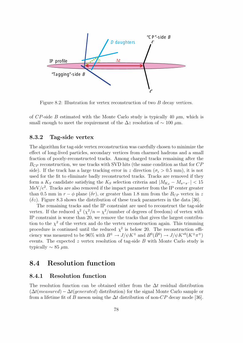
–
IP profile
D daughters
D
“CP”-side B
+
“Tagging”-side B
∆z
Figure 8.2: Illustration for vertex reconstruction of two B decay vertices.
of CP -side B estimated with the Monte Carlo study is typically 40 µm, which issmall enough to meet the requirement of the ∆z resolution of ∼ 100 µm.
8.3.2 Tag-side vertex
The algorithm for tag-side vertex reconstruction was carefully chosen to minimize theeffect of long-lived particles, secondary vertices from charmed hadrons and a smallfraction of poorly-reconstructed tracks. Among charged tracks remaining after theBCP reconstruction, we use tracks with SVD hits (the same condition as that for CPside). If the track has a large tracking error in z direction (σz > 0.5 mm), it is notused for the fit to eliminate badly reconstructed tracks. Tracks are removed if theyform a KS candidate satisfying the KS selection criteria and |MKS
−Mπ+π−| < 15MeV/c2. Tracks are also removed if the impact parameter from the IP center greaterthan 0.5 mm in r − φ plane (δr), or greater than 1.8 mm from the BCP vertex in z(δz). Figure 8.3 shows the distribution of these track parameters in the data [36].
The remaining tracks and the IP constraint are used to reconstruct the tag-sidevertex. If the reduced χ2 (χ2/n = χ2/number of degrees of freedom) of vertex withIP constraint is worse than 20, we remove the tracks that gives the largest contribu-tion to the χ2 of the vertex and do the vertex reconstruction again. This trimmingprocedure is continued until the reduced χ2 is below 20. The reconstruction effi-ciency was measured to be 96% with B± → J/ψK± and B0(B0) → J/ψK∗0(K±π∓)events. The expected z vertex resolution of tag-side B with Monte Carlo study istypically ∼ 85 µm.
8.4 Resolution function
8.4.1 Resolution function
The resolution function can be obtained either from the ∆t residual distribution(∆t(measured)−∆t(generated) distribution) for the signal Monte Carlo sample orfrom a lifetime fit of B meson using the ∆t distribution of non-CP decay mode [36].
78

σz (µm)track
0
10
20
30
40
50
0 200 400 600 800 1000
δz (µm)
0
10
20
30
40
50
60
-2000 0 2000δr (µm)
0
10
20
30
40
50
-1000 -500 0 500 1000
(a)
(c)(b)
[Ent
ries/
10µm
]
[Ent
ries/
20µm
]
[Ent
ries/
50µm
]
Figure 8.3: (a) σtrackz distribution, (b) δz distribution and (c) δr distribution in thedata. Vertical line indicate cut values for each variable.
The resolution of ∆t, R(∆t), is parametrized as a sum of two Gaussians, wherea main Gaussian is for the intrinsic SVD resolution and the effect of the secondarycharmed mesons in tag-side B decays, and a tail Gaussian is for a few poorly recon-structed tracks :
R(∆t) =fmain
σ√
2πexp
(−(∆t− µ)2
2σ2
)+
ftail
σtail√
2πexp
(−(∆t− µtail)
2
2σ2tail
). (8.9)
The mean values (µ, µtail) and width (σ, σtail) of the two Gaussians are calculatedevent-by-event from the CP -side and tag-side vertex errors, taking into account theerror due to the approximation of ∆t ∼ ∆z/βγc. The Gaussian parameters andthe fraction ftail (= 1− fmain) are determined from the full Monte Carlo simulationstudies and a multi-parameter fit to B → D∗ν data. Figure 8.4 shows the exampleof average shape of the R(∆t) by summing event-by-event R(∆t) functions over440 B− → D0π− events. In order to parameterize the total shape of the averagedresolution function, we fit it by a triple Gaussian. The following function is obtainedby the fit, and we use this function as the resolution function in this analysis.
g(∆t− ∆t′) = 0.656e−(∆t−∆t′+0.143)2
2×0.7542 + 0.298e−(∆t−∆t′+0.260)2
2×1.652 + 0.046e−(∆t−∆t′+0.56)2
2×0.4.72 .(8.10)
79
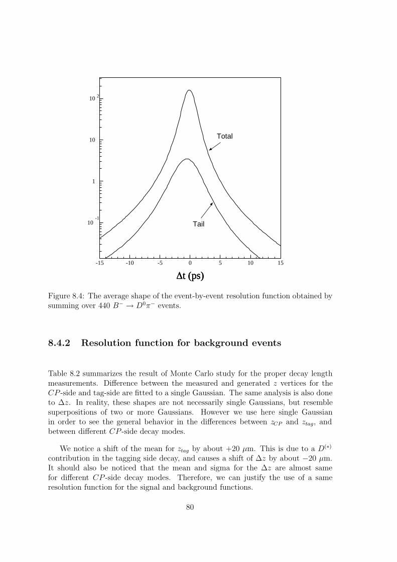
Total
Tail10-1
1
10
10 2
-15 -10 -5 0 5 10 15
∆t (ps)∆t (ps)∆t (ps)
Figure 8.4: The average shape of the event-by-event resolution function obtained bysumming over 440 B− → D0π− events.
8.4.2 Resolution function for background events
Table 8.2 summarizes the result of Monte Carlo study for the proper decay lengthmeasurements. Difference between the measured and generated z vertices for theCP -side and tag-side are fitted to a single Gaussian. The same analysis is also doneto ∆z. In reality, these shapes are not necessarily single Gaussians, but resemblesuperpositions of two or more Gaussians. However we use here single Gaussianin order to see the general behavior in the differences between zCP and ztag, andbetween different CP -side decay modes.
We notice a shift of the mean for ztag by about +20 µm. This is due to a D(∗)
contribution in the tagging side decay, and causes a shift of ∆z by about −20 µm.It should also be noticed that the mean and sigma for the ∆z are almost samefor different CP -side decay modes. Therefore, we can justify the use of a sameresolution function for the signal and background functions.
80
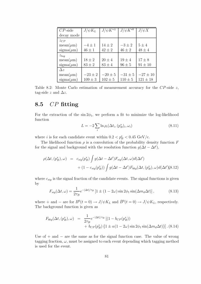
CP -side J/ψKL J/ψK∗± J/ψK∗0 J/ψXdecay modezCPmean(µm) −4 ± 1 14 ± 2 −3 ± 2 5 ± 4sigma(µm) 46 ± 1 42 ± 2 46 ± 2 48 ± 4ztagmean(µm) 18 ± 2 20 ± 4 19 ± 4 17 ± 8sigma(µm) 83 ± 2 83 ± 4 96 ± 5 91 ± 10∆zmean(µm) −23 ± 2 −20 ± 5 −31 ± 5 −27 ± 10sigma(µm) 109 ± 3 102 ± 5 110 ± 5 121 ± 18
Table 8.2: Monte Carlo estimation of measurement accuracy for the CP -side z,tag-side z and ∆z.
8.5 CP fitting
For the extraction of the sin 2φ1, we perform a fit to minimize the log-likelihoodfunction
L = −2∑i
ln ρi(∆ti, (p∗B)i, ωi) (8.11)
where i is for each candidate event within 0.2 < p∗B < 0.45 GeV/c.
The likelihood function ρ is a convolution of the probability density function Ffor the signal and background with the resolution function g(∆t− ∆t′),
ρ(∆t, (p∗B), ω) = csig(p∗B)∫g(∆t− ∆t′)Fsig(∆t, ω)d(∆t′)
+ (1 − csig(p∗B))
∫g(∆t− ∆t′)Fbkg(∆t, (p∗B), ω)d(∆t′),(8.12)
where csig is the signal fraction of the candidate events. The signal functions is givenby
Fsig(∆t, ω) =1
2τBe−|∆t|/τB [1 ± (1 − 2ω) sin 2φ1 sin(∆md∆t)] , (8.13)
where + and − are for B0(t = 0) → J/ψKL and B0(t = 0) → J/ψKL, respectively.The background function is given as
Fbkg(∆t, (p∗B), ω) =
1
2τBe−|∆t|/τB [(1 − bCP (p∗B))
+ bCP (p∗B) 1 ± α(1 − 2ω) sin 2φ1 sin(∆md∆t)] . (8.14)
Use of + and − are the same as for the signal function case. The value of wrongtagging fraction, ω, must be assigned to each event depending which tagging methodis used for the event.
81
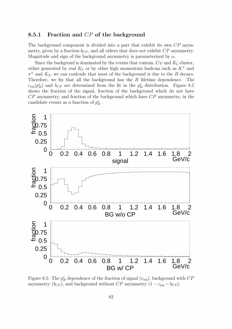
8.5.1 Fraction and CP of the background
The background component is divided into a part that exhibit its own CP asym-metry, given by a fraction bCP , and all others that does not exhibit CP asymmetry.Magnitude and sign of the background asymmetry is parameterized by α.
Since the backgrond is dominated by the events that contain J/ψ and KL cluster,either generated by real KL or by other high momentum hadrons such as K± andπ± and KS, we can conlcude that most of the background is due to the B decays.Therefore, we fix that all the background has the B lifetime dependence. Thecsig(p
∗B) and bCP are determined from the fit in the p∗B distribution. Figure 8.5
shows the fraction of the signal, fraction of the background which do not haveCP asymmetry, and fraction of the background which have CP asymmetry, in thecandidate events as a function of p∗B .
00.25
0.50.75
1
0 0.2 0.4 0.6 0.8 1 1.2 1.4 1.6 1.8 2signal GeV/c
frac
tion
00.25
0.50.75
1
0 0.2 0.4 0.6 0.8 1 1.2 1.4 1.6 1.8 2BG w/o CP GeV/c
frac
tion
00.25
0.50.75
1
0 0.2 0.4 0.6 0.8 1 1.2 1.4 1.6 1.8 2BG w/ CP GeV/c
frac
tion
Figure 8.5: The p∗B dependence of the fraction of signal (csig), background with CPasymmetry (bCP ), and background without CP asymmetry (1 − csig − bCP ).
82
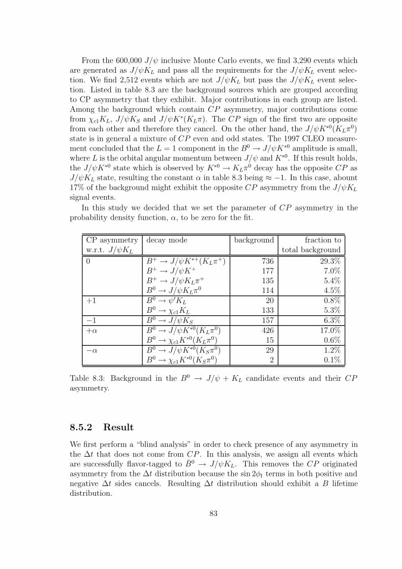
From the 600,000 J/ψ inclusive Monte Carlo events, we find 3,290 events whichare generated as J/ψKL and pass all the requirements for the J/ψKL event selec-tion. We find 2,512 events which are not J/ψKL but pass the J/ψKL event selec-tion. Listed in table 8.3 are the background sources which are grouped accordingto CP asymmetry that they exhibit. Major contributions in each group are listed.Among the background which contain CP asymmetry, major contributions comefrom χc1KL, J/ψKS and J/ψK∗(KLπ). The CP sign of the first two are oppositefrom each other and therefore they cancel. On the other hand, the J/ψK∗0(KLπ
0)state is in general a mixture of CP even and odd states. The 1997 CLEO measure-ment concluded that the L = 1 component in the B0 → J/ψK∗0 amplitude is small,where L is the orbital angular momentum between J/ψ and K∗0. If this result holds,the J/ψK∗0 state which is observed by K∗0 → KLπ
0 decay has the opposite CP asJ/ψKL state, resulting the constant α in table 8.3 being ≈ −1. In this case, abount17% of the background might exhibit the opposite CP asymmetry from the J/ψKL
signal events.
In this study we decided that we set the parameter of CP asymmetry in theprobability density function, α, to be zero for the fit.
CP asymmetry decay mode background fraction tow.r.t. J/ψKL total background
0 B+ → J/ψK∗+(KLπ+) 736 29.3%
B+ → J/ψK+ 177 7.0%B+ → J/ψKLπ
+ 135 5.4%B0 → J/ψKLπ
0 114 4.5%+1 B0 → ψ′KL 20 0.8%
B0 → χc1KL 133 5.3%−1 B0 → J/ψKS 157 6.3%+α B0 → J/ψK∗0(KLπ
0) 426 17.0%B0 → χc1K
∗0(KLπ0) 15 0.6%
−α B0 → J/ψK∗0(KSπ0) 29 1.2%
B0 → χc1K∗0(KSπ
0) 2 0.1%
Table 8.3: Background in the B0 → J/ψ + KL candidate events and their CPasymmetry.
8.5.2 Result
We first perform a “blind analysis” in order to check presence of any asymmetry inthe ∆t that does not come from CP . In this analysis, we assign all events whichare successfully flavor-tagged to B0 → J/ψKL. This removes the CP originatedasymmetry from the ∆t distribution because the sin 2φ1 terms in both positive andnegative ∆t sides cancels. Resulting ∆t distribution should exhibit a B lifetimedistribution.
83
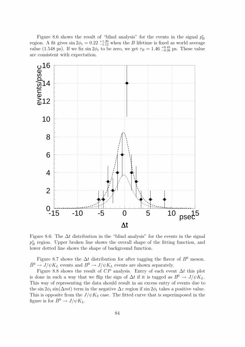
Figure 8.6 shows the result of “blind analysis” for the events in the signal p∗Bregion. A fit gives sin 2φ1 = 0.22 +1.20
−1.12 when the B lifetime is fixed as world averagevalue (1.548 ps). If we fix sin 2φ1 to be zero, we get τB = 1.46 +0.45
−0.38 ps. These valueare consistent with expectation.
0
2
4
6
8
10
12
14
16
-15 -10 -5 0 5 10 15
∆tpsec
even
ts/p
sec
∆t∆tFigure 8.6: The ∆t distribution in the “blind analysis” for the events in the signalp∗B region. Upper broken line shows the overall shape of the fitting function, andlower dotted line shows the shape of background function.
Figure 8.7 shows the ∆t distribution for after tagging the flavor of B0 meson.B0 → J/ψKL events and B0 → J/ψKL events are shown separately.
Figure 8.8 shows the result of CP analysis. Entry of each event ∆t this plotis done in such a way that we flip the sign of ∆t if it is tagged as B0 → J/ψKL.This way of representing the data should result in an excess entry of events due tothe sin 2φ1 sin(∆mt) term in the negative ∆z region if sin 2φ1 takes a positive value.This is opposite from the J/ψKS case. The fitted curve that is superimposed in thefigure is for B0 → J/ψKL.
84

While the fitting is done properly, the CP -dependent ∆t shape for the B0 →J/ψKL sample with their ∆t sign being flipped is not completely identical to thatof the B0 → J/ψKL sample. This is because a small shift in the ∆t distribution dueto the D∗ contribution occurs toward the negative side for both cases and flipping ofthe ∆t sign causes a flip of this shift also. However, the 20 µm shift corresponds toabout 0.16 ps shift, and too small to be noticeable with the present level of statistics.
A fit gives sin 2φ1 = −1.00 +0.89−0.73 when the τB is fixed at the world average value.
85
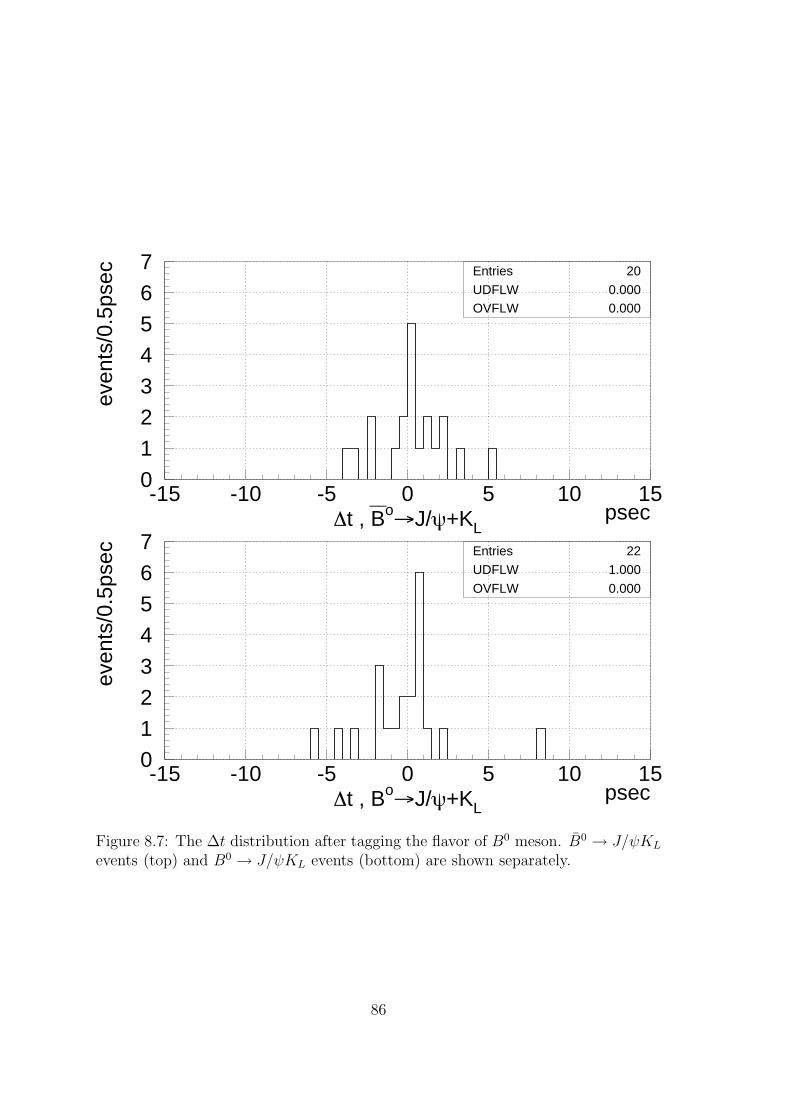
0
1234567
-15 -10 -5 0 5 10 15
Entries
UDFLWOVFLW
20
0.000 0.000
∆t , B⎯o→J/ψ+KL
psec
even
ts/0
.5ps
ec
0123
4567
-15 -10 -5 0 5 10 15
Entries
UDFLW
OVFLW
22
1.000
0.000
∆t , Bo→J/ψ+KLpsec
even
ts/0
.5ps
ec
Figure 8.7: The ∆t distribution after tagging the flavor of B0 meson. B0 → J/ψKL
events (top) and B0 → J/ψKL events (bottom) are shown separately.
86
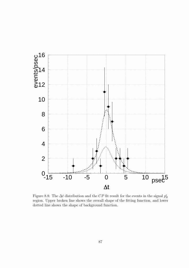
0
2
4
6
8
10
12
14
16
-15 -10 -5 0 5 10 15
∆tpsec
even
ts/p
sec
∆t∆tFigure 8.8: The ∆t distribution and the CP fit result for the events in the signal p∗Bregion. Upper broken line shows the overall shape of the fitting function, and lowerdotted line shows the shape of background function.
87
Chapter 9
Conclusion
We have measured the CP asymmetry parameter sin 2φ1 in the B0 → J/ψ + KL
decay.
For the detection of KL and muons, the KLM detector subsystem was con-structed which was based on glass-electrode resistive plate chambers (RPC). Thesuperlayer structure and independent gas/HV lines for each detector module pro-vides a stable and reliable operation. Although this was the first time that the glassplates were used as the RPC electrode, the performance of the system under thehigh luminosity runs was proved to be excellent.
We measured the KL by finding the hadron showers with the combination of theKLM and the electromagnetic calorimeter. Only the KL direction was measured inthis experiment. The magnitude of KL momentum was determined by the measuredJ/ψ momentum and KL angle, and assuming the two body decay. The B0 →J/ψ+KL signal was extracted from the center-of-mass momentum spectrum of theparent B0.
We used the first data set taken by the Belle detector at KEK B-factory fromJune 1999 to July 2000. The total integrated luminosity of 6.2 fb−1 is accumulatedon the energy of Υ(4S) resonance. We observed 102 candidate of B0 → J/ψ +KL
events in total, where 48 events are estimated to be the background events from thefitting results for the shape of p∗B distribution obtained by Monte Carlo simulationstudy. This is the first direct observation of the B0 → J/ψ+KL decays. We observeabout 20% discrepancy of the KL yield between data and Monte Carlo. Study ofhadron shower formation in the detector using charged pions and kaons in the datashowed that the Monte Carlo might not be representing the real data correctly.
We could successfully identify the flavor of B mesons by either high momentumlepton, kaon of all momentum range, mid-momentum lepton, and slow pion. Wecould also measure the distance between two B meson vertices with the silicon vertexdetector. A total of 42 events remained out of 102 events after the flavor taggingwas done.
Although statistic is limited, from the fitting to the proper time distribution ofthe 42 events we obtained the value
sin 2φ1 = −1.00 +0.89−0.73. (9.1)
88

It should be noted that the discrepancy in the KL detection efficiency which weobserve between Data and Monte Carlo has no effect for the sin 2φ1 measurementsince it depends only on the ∆t distribution in B0 → J/ψKL events and B0 →J/ψKL events.
The current preliminary result of sin 2φ1 value of Belle experiment, which isthe combined result of fitting to the J/ψKS, ψ(2S)KS, χc1KS, J/ψπ
0 and J/ψKL
(98 events in total), is sin 2φ1 = 0.45 +0.43−0.44(stat)
+0.07−0.09(syst). The sin 2φ1 value of
B0 → J/ψ+KL mode alone has the opposite sign from the combined result. It shouldhave the same value as that from other channels based on our formalism. We believethat this is a result of statistical fluctuation due to small event sample. However, thisanalysis demonstrated that we can extract sin 2φ1 value from the B0 → J/ψ +KL
mode. As we accumulate more event sample, an accurate determination of sin 2φ1
should follow.
89
Appendix A
J/ψK∗(KLπ) reduction
In this chapter we describe the study for the reduction of J/ψK∗(KLπ) backgroundevents. We tried to reduce the background which comes from B → J/ψK∗(KLπ)by attempting to reconstruct positively the K∗ → KLπ for the events which remainin the signal region.
A.1 B− → J/ψK∗−(KLπ−)
We add all available π− in the event with J/ψ and KL one by one, and computethe p∗B assuming 3-body decay. We also compute the mKπ assuming 3-body decay.Figure A.1 shows a result of this study with Monte Carlo sample, which is summa-rized in Table A.1. Although simple one-dimensional cuts on p∗B or mKπ assuming3-body decay reduces the background significantly, they also lower the efficiency forthe signal events. The box cut of p∗B and mKπ, on the other hand, reduces thebackground by half while lowering the signal efficiency by only 16%.
We tried further reduction of this background by using the vertex information.The z vertex of π− tracks should coincide with that of J/ψ if the pion track originatesfrom K∗−, whereas the pion in the J/ψKL events should have no correlation. Weselect “good pions” by making a cut on the confidence level of a fit which tries tofind a common vertex between J/ψ and pion. Table A.2 summarizes the result ofthis study. The signal to background ratio is worse when the vertex information isadded and the Figure Of Merit (F.O.M) shows hardly an improvement. Our vertexresolution is not good enough for this purpose.
A.2 B0 → J/ψK∗0(KLπ0)
We repeated an analysis described in the previous section to reduce the J/ψK∗0
(KLπ0) background. Figure A.2 shows p∗B vs mKπ plot for this study. Table A.3
summarizes the result. The result is almost same as that in B− → J/ψK∗−(KLπ−)
reduction.
90
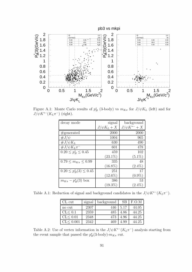
pb3 vs mkpi
00.20.40.60.8
11.21.41.61.8
2
0 0.5 1 1.5 2
ID 121ENTRIES 438 0.00 3.00 2.00
0.00 433. 0.00 0.00 0.00 0.00
J/ψKL
MKπ(GeV/c2)
P* B(
3)(G
eV/c
)
00.20.40.60.8
11.21.41.61.8
2
0 0.5 1 1.5 2
ID 121ENTRIES 99 0.00 0.00 0.00
0.00 99.0 0.00 0.00 0.00 0.00
J/ψK*±MKπ(GeV/c2)
P* B(
3)(G
eV/c
)Figure A.1: Monte Carlo results of p∗B (3-body) vs mKπ for J/ψKL (left) and forJ/ψK∗−(KLπ
−) (right).
decay mode signal backgroundJ/ψKL +X J/ψK∗− +X
#generated 2000 2000#J/ψ 1004 965#J/ψKL 630 490#J/ψKLπ
− 601 4780.20 ≤ p∗B ≤ 0.45 459 102
(23.1%) (5.1%)0.79 ≤ mKπ ≤ 0.99 335 48
(16.8%) (2.4%)0.20 ≤ p∗B(3) ≤ 0.45 251 17
(12.6%) (0.9%)mKπ − p∗B(3) box 386 53
(19.3%) (2.4%)
Table A.1: Reduction of signal and background candidates in the J/ψK∗−(KLπ−).
CL cut signal background SB F.O.M
no cut 2307 446 5.17 44.05CL≤ 0.1 2359 485 4.86 44.25CL≤ 0.01 2348 473 4.96 44.25CL≤ 0.001 2342 469 4.99 44.25
Table A.2: Use of vertex information in the J/ψK∗−(KLπ−) analysis starting from
the event sample that passed the p∗B(3-body)-mKπ cut.
91
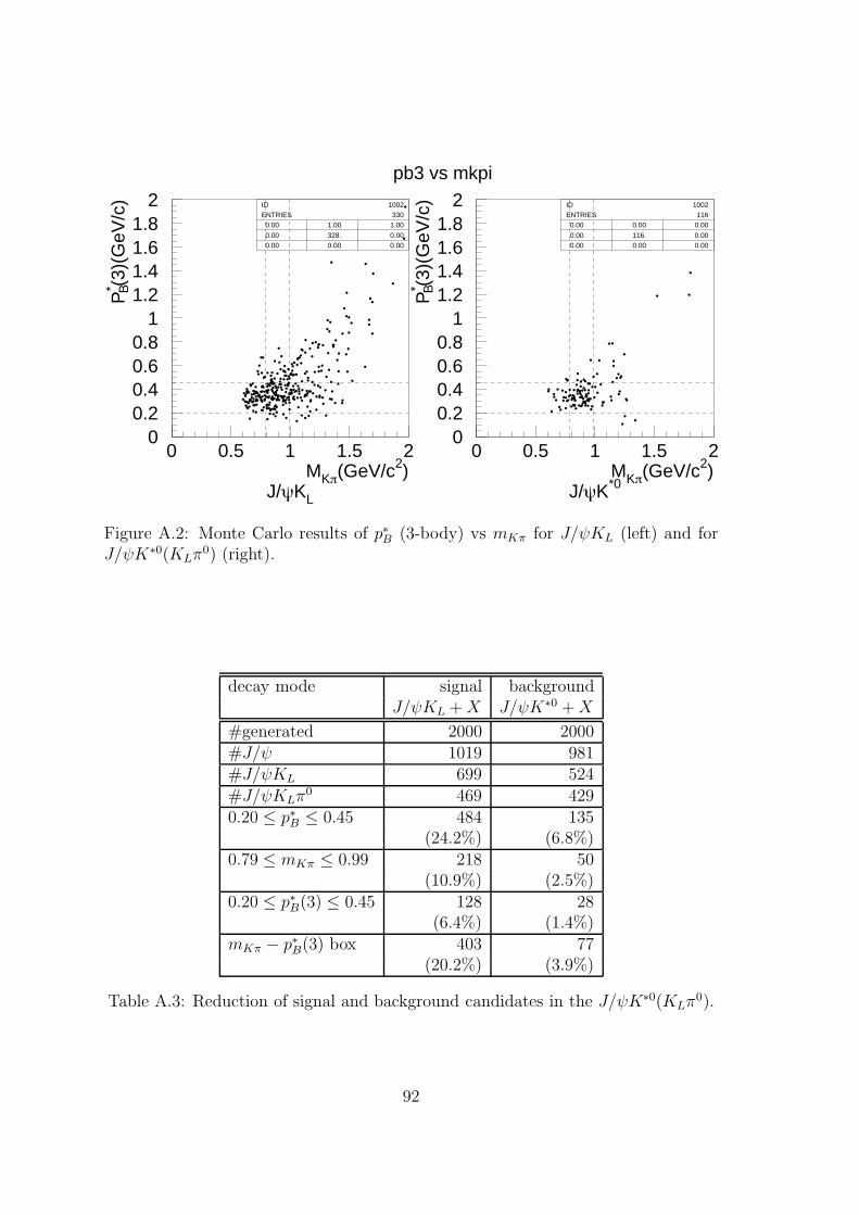
pb3 vs mkpi
00.20.40.60.8
11.21.41.61.8
2
0 0.5 1 1.5 2
ID 1002ENTRIES 330 0.00 1.00 1.00
0.00 328. 0.00 0.00 0.00 0.00
J/ψKL
MKπ(GeV/c2)
P* B(
3)(G
eV/c
)
00.20.40.60.8
11.21.41.61.8
2
0 0.5 1 1.5 2
ID 1002ENTRIES 116 0.00 0.00 0.00
0.00 116. 0.00 0.00 0.00 0.00
J/ψK*0MKπ(GeV/c2)
P* B(
3)(G
eV/c
)
Figure A.2: Monte Carlo results of p∗B (3-body) vs mKπ for J/ψKL (left) and forJ/ψK∗0(KLπ
0) (right).
decay mode signal backgroundJ/ψKL +X J/ψK∗0 +X
#generated 2000 2000#J/ψ 1019 981#J/ψKL 699 524#J/ψKLπ
0 469 4290.20 ≤ p∗B ≤ 0.45 484 135
(24.2%) (6.8%)0.79 ≤ mKπ ≤ 0.99 218 50
(10.9%) (2.5%)0.20 ≤ p∗B(3) ≤ 0.45 128 28
(6.4%) (1.4%)mKπ − p∗B(3) box 403 77
(20.2%) (3.9%)
Table A.3: Reduction of signal and background candidates in the J/ψK∗0(KLπ0).
92

A.3 Summary
Although the box cut of p∗B and mKπ assuming 3-body decay removes a significantfraction of the J/ψK∗(KLπ) background, we did not use it in this analysis. This isbecause a limited statistics of the data sample does not allow a reliable examinationof the performance of this method, and we must rely entirely on the Monte Carlostudy.
93

Bibliography
[1] J. H. Christensen et al., Phys. Rev. Lett. 13 (1964) 138.
[2] M. Kobayashi and T. Maskawa, Prog. Theo. Phys 49 (1973) 652.
[3] J. E. Augustin et al., Phys. Rev. Lett. 33 (1974) 1406.
[4] J. J. Aubert et al., Phys. Rev. Lett. 33 (1974) 1404.
[5] S. W. Herb et al., Phys. Rev. Lett. 39 (1977) 252.
[6] A.Carter and A.I.Sanda, Phys.Rev.Lett. 45(1980)952;Phys.Rev.D23,1567(1981);I. I. Bigi and A. I. Sanda, Nucl. Phys. 193,851(1981).
[7] E. Fernandez et al.(MAC), Phys. Rev. Lett. 51 (1983) 1022;N. Lockyer et al.(MARKII), Phys. Rev. Lett. 51 (1983) 1316.
[8] The BaBar collaboration, Technical Design Report, (1995).
[9] F.Abe et al.(CDF collaboration), Phys. Rev. Lett. 81 (1998) 5513.
[10] LHC-B Letter of Intent, CERN/LHCC 95-5, LHCC/18, August 1995.
[11] S.Weinberg : Phys.Rev.Lett. Phys. Rev. Lett. 19 (1967) 1264,A.Salam : Elementary Particle physics, ed. N.Svartholm (Almquist and Wik-sells, Stockholm 1968) 367.
[12] L.Wolfenstein, Phys. Rev. Lett. 51 (1983) 1945.
[13] C.Caso et al., [Particle Data Group], Eur. Phys. J. C3, 1 (1998).
[14] R.Aleksan, to appear in: Proceedings of the International Europhisics Confer-ence on High Energy Physics, Brussels, Belgium, September 1995.
[15] KEKB B-factory design report, KEK Report 95-3, 1995.
[16] BELLE SVD group, Technical design report of BELLE SVD, 1998.
[17] S.K. Sahu et al., BELLE Note 203 (1997).
[18] A. Abashian et al., Nucl. Instr. and Meth. A449 (2000) 112.
[19] M. Sanpei et al., IEEE Trans. Nucl. Sci. Vol.44, No.3, 752(1997).
94
[20] R. Itoh and S. Ichizawa, BELLE Note 97 (1995).
[21] S. Nagayama, PANTHER — User’s guide —, Version 3.0 (1997).
[22] A. Putzer, Comput. Phys. Commun. 57,156(1989).
[23] K.Hanagaki et al., BELLE Note 312 (2000).
[24] L.Piilonen et al., BELLE Note 338 (2000).
[25] KID group, BELLE Note 321 (2000).
[26] CLEO software document homepage :http://www.lns.cornell.edu/public/CLEO/soft/QQ/index.html (1998).
[27] R. Itoh, QQ quick reference for BELLE (1995).
[28] T.Sjostrand, “PYTHIA 5.7 and JETSET 7.4 Physics and Manual”, CERN-TH.7112/93 (1993).
[29] “GEANT” Detector Description and Simulation Tool, CERN program LibraryLong Writeup W5013 (1993).
[30] H. Ozaki, BELLE Note 99 (1996).
[31] S. Azuchi et al., BELLE Note 265 (1999).
[32] S. Azuchi, Master thesis, Tohoku University, February, 2000.
[33] S. Kumar, BELLE Note 351 (2000).
[34] G. Fox and S. Wolfram, Phys. Rev. Lett. 41 (1978) 1581.
[35] J. Suzuki, BELLE Note 313 (2000).
[36] T.Nakadaira et al., BELLE Note 290 (2000).
95