Measure theory and probability

Alexander GrigoryanUniversity of Bielefeld

Lecture Notes, October 2007 - February 2008

Contents

1 Construction of measures 31.1 Introduction and examples . . . . . . . . . . . . . . . . . . . . . . . . . . . 31.2 σ-additive measures . . . . . . . . . . . . . . . . . . . . . . . . . . . . . . . 51.3 An example of using probability theory . . . . . . . . . . . . . . . . . . . . 71.4 Extension of measure from semi-ring to a ring . . . . . . . . . . . . . . . . 81.5 Extension of measure to a σ-algebra . . . . . . . . . . . . . . . . . . . . . . 11

1.5.1 σ-rings and σ-algebras . . . . . . . . . . . . . . . . . . . . . . . . . 111.5.2 Outer measure . . . . . . . . . . . . . . . . . . . . . . . . . . . . . 131.5.3 Symmetric difference . . . . . . . . . . . . . . . . . . . . . . . . . . 141.5.4 Measurable sets . . . . . . . . . . . . . . . . . . . . . . . . . . . . . 16

1.6 σ-finite measures . . . . . . . . . . . . . . . . . . . . . . . . . . . . . . . . 201.7 Null sets . . . . . . . . . . . . . . . . . . . . . . . . . . . . . . . . . . . . . 231.8 Lebesgue measure in Rn . . . . . . . . . . . . . . . . . . . . . . . . . . . . 25

1.8.1 Product measure . . . . . . . . . . . . . . . . . . . . . . . . . . . . 251.8.2 Construction of measure in Rn. . . . . . . . . . . . . . . . . . . . . 26

1.9 Probability spaces . . . . . . . . . . . . . . . . . . . . . . . . . . . . . . . . 281.10 Independence . . . . . . . . . . . . . . . . . . . . . . . . . . . . . . . . . . 29

2 Integration 382.1 Measurable functions . . . . . . . . . . . . . . . . . . . . . . . . . . . . . . 382.2 Sequences of measurable functions . . . . . . . . . . . . . . . . . . . . . . . 422.3 The Lebesgue integral for finite measures . . . . . . . . . . . . . . . . . . . 47

2.3.1 Simple functions . . . . . . . . . . . . . . . . . . . . . . . . . . . . 472.3.2 Positive measurable functions . . . . . . . . . . . . . . . . . . . . . 492.3.3 Integrable functions . . . . . . . . . . . . . . . . . . . . . . . . . . . 52

2.4 Integration over subsets . . . . . . . . . . . . . . . . . . . . . . . . . . . . 562.5 The Lebesgue integral for σ-finite measure . . . . . . . . . . . . . . . . . . 592.6 Convergence theorems . . . . . . . . . . . . . . . . . . . . . . . . . . . . . 612.7 Lebesgue function spaces Lp . . . . . . . . . . . . . . . . . . . . . . . . . . 68

2.7.1 The p-norm . . . . . . . . . . . . . . . . . . . . . . . . . . . . . . . 692.7.2 Spaces Lp . . . . . . . . . . . . . . . . . . . . . . . . . . . . . . . . 71

2.8 Product measures and Fubini’s theorem . . . . . . . . . . . . . . . . . . . . 762.8.1 Product measure . . . . . . . . . . . . . . . . . . . . . . . . . . . . 76

1

2.8.2 Cavalieri principle . . . . . . . . . . . . . . . . . . . . . . . . . . . . 782.8.3 Fubini’s theorem . . . . . . . . . . . . . . . . . . . . . . . . . . . . 83

3 Integration in Euclidean spaces and in probability spaces 863.1 Change of variables in Lebesgue integral . . . . . . . . . . . . . . . . . . . 863.2 Random variables and their distributions . . . . . . . . . . . . . . . . . . . 1003.3 Functionals of random variables . . . . . . . . . . . . . . . . . . . . . . . . 1043.4 Random vectors and joint distributions . . . . . . . . . . . . . . . . . . . . 1063.5 Independent random variables . . . . . . . . . . . . . . . . . . . . . . . . . 1103.6 Sequences of random variables . . . . . . . . . . . . . . . . . . . . . . . . . 1143.7 The weak law of large numbers . . . . . . . . . . . . . . . . . . . . . . . . 1153.8 The strong law of large numbers . . . . . . . . . . . . . . . . . . . . . . . . 1173.9 Extra material: the proof of the Weierstrass theorem using the weak law

of large numbers . . . . . . . . . . . . . . . . . . . . . . . . . . . . . . . . 121

2

1 Construction of measures

1.1 Introduction and examples

The main subject of this lecture course and the notion of measure (Maß). The rigorousdefinition of measure will be given later, but now we can recall the familiar from theelementary mathematics notions, which are all particular cases of measure:1. Length of intervals in R: if I is a bounded interval with the endpoints a, b (that is,

I is one of the intervals (a, b), [a, b], [a, b), (a, b]) then its length is defined by

(I) = |b− a| .

The useful property of the length is the additivity: if an interval I is a disjoint union ofa finite family Iknk=1 of intervals, that is, I =

Fk Ik, then

(I) =nX

k=1

(Ik) .

Indeed, let aiNi=0 be the set of all distinct endpoints of the intervals I, I1, ..., In enumer-ated in the increasing order. Then I has the endpoints a0, aN while each interval Ik hasnecessarily the endpoints ai, ai+1 for some i (indeed, if the endpoints of Ik are ai and ajwith j > i+1 then the point ai+1 is an interior point of Ik, which means that Ik must in-tersect with some other interval Im). Conversely, any couple ai, ai+1 of consecutive pointsare the end points of some interval Ik (indeed, the interval (ai, ai+1) must be covered bysome interval Ik; since the endpoints of Ik are consecutive numbers in the sequence aj,it follows that they are ai and ai+1). We conclude that

(I) = aN − a0 =N−1Xi=0

(ai+1 − ai) =nX

k=1

(Ik) .

2. Area of domains in R2. The full notion of area will be constructed within thegeneral measure theory later in this course. However, for rectangular domains the area isdefined easily. A rectangle A in R2 is defined as the direct product of two intervals I, Jfrom R:

A = I × J =©(x, y) ∈ R2 : x ∈ I, y ∈ J

ª.

Then setarea (A) = (I) (J) .

We claim that the area is also additive: if a rectangle A is a disjoint union of a finitefamily of rectangles A1, ..., An, that is, A =

Fk Ak, then

area (A) =nX

k=1

area (Ak) .

For simplicity, let us restrict the consideration to the case when all sides of all rectanglesare semi-open intervals of the form [a, b). Consider first a particular case, when the

3

rectangles A1, ..., Ak form a regular tiling of A; that is, let A = I ×J where I =F

i Ii andJ =

Fj Jj, and assume that all rectangles Ak have the form Ii × Jj. Then

area (A) = (I) (J) =Xi

(Ii)Xj

(Jj) =Xi,j

(Ii) (Jj) =Xk

area (Ak) .

Now consider the general case when A is an arbitrary disjoint union of rectangles Ak.Let xi be the set of all X-coordinates of the endpoints of the rectangles Ak put inthe increasing order, and yj be similarly the set of all the Y -coordinates, also in theincreasing order. Consider the rectangles

Bij = [xi, xi+1)× [yj, yj+1).

Then the family Biji,j forms a regular tiling of A and, by the first case,

area (A) =Xi,j

area (Bij) .

On the other hand, each Ak is a disjoint union of some of Bij, and, moreover, those Bij

that are subsets of Ak, form a regular tiling of Ak, which implies that

area(Ak) =X

Bij⊂Ak

area (Bij) .

Combining the previous two lines and using the fact that each Bij is a subset of exactlyone set Ak, we obtainX

k

area (Ak) =Xk

XBij⊂Ak

area (Bij) =Xi,j

area (Bij) = area (A) .

3. Volume of domains in R3. The construction is similar to the area. Consider allboxes in R3, that is, the domains of the form A = I × J ×K where I, J,K are intervalsin R, and set

vol (A) = (I) (J) (K) .

Then volume is also an additive functional, which is proved in a similar way. Later on,we will give the detailed proof of a similar statement in an abstract setting.4. Probability is another example of an additive functional. In probability theory,

one considers a set Ω of elementary events, and certain subsets of Ω are called events(Ereignisse). For each event A ⊂ Ω, one assigns the probability, which is denoted byP (A) and which is a real number in [0, 1]. A reasonably defined probability must satisfythe additivity: if the event A is a disjoint union of a finite sequence of evens A1, ..., An

then

P (A) =nX

k=1

P (Ak) .

The fact that Ai and Aj are disjoint, when i 6= j, means that the events Ai and Aj cannotoccur at the same time.The common feature of all the above example is the following. We are given a non-

empty setM (which in the above example was R, R2, R3, Ω), a family S of its subsets (the

4

families of intervals, rectangles, boxes, events), and a functional μ : S → R+ := [0,+∞)(length, area, volume, probability) with the following property: if A ∈ S is a disjointunion of a finite family Aknk=1 of sets from S then

μ (A) =nX

k=1

μ (Ak) .

A functional μ with this property is called a finitely additive measure. Hence, length,area, volume, probability are all finitely additive measures.

1.2 σ-additive measures

As above, let M be an arbitrary non-empty set and S be a family of subsets of M .

Definition. A functional μ : S → R+ is called a σ-additive measure if whenever a setA ∈ S is a disjoint union of an at most countable sequence AkNk=1 (where N is eitherfinite or N =∞) then

μ (A) =NXk=1

μ (Ak) .

If N = ∞ then the above sum is understood as a series. If this property holds only forfinite values of N then μ is a finitely additive measure.

Clearly, a σ-additive measure is also finitely additive (but the converse is not true).At first, the difference between finitely additive and σ-additive measures might look in-significant, but the σ-additivity provides much more possibilities for applications and isone of the central issues of the measure theory. On the other hand, it is normally moredifficult to prove σ-additivity.

Theorem 1.1 The length is a σ-additive measure on the family of all bounded intervalsin R.

Before we prove this theorem, consider a simpler property.

Definition. A functional μ : S → R+ is called σ-subadditive if whenever A ⊂SN

k=1Ak

where A and all Ak are elements of S and N is either finite or infinite, then

μ (A) ≤NXk=1

μ (Ak) .

If this property holds only for finite values of N then μ is called finitely subadditive.

Lemma 1.2 The length is σ-subadditive.

Proof. Let I, Ik∞k=1 be intervals such that I ⊂S∞

k=1 Ik and let us prove that

(I) ≤∞Xk=1

(Ik)

5

(the case N <∞ follows from the case N =∞ by adding the empty interval). Let us fixsome ε > 0 and choose a bounded closed interval I 0 ⊂ I such that

(I) ≤ (I 0) + ε.

For any k, choose an open interval I 0k ⊃ Ik such that

(I 0k) ≤ (Ik) +ε

2k.

Then the bounded closed interval I 0 is covered by a sequence I 0k of open intervals. Bythe Borel-Lebesgue lemma, there is a finite subfamily

nI 0kj

onj=1

that also covers I 0. It

follows from the finite additivity of length that it is finitely subadditive, that is,

(I 0) ≤Xj

(I 0kj),

(see Exercise 7), which implies that

(I 0) ≤∞Xk=1

(I 0k) .

This yields

l (I) ≤ ε+∞Xk=1

³(Ik) +

ε

2k

´= 2ε+

∞Xk=1

(Ik) .

Since ε > 0 is arbitrary, letting ε→ 0 we finish the proof.Proof of Theorem 1.1. We need to prove that if I =

F∞k=1 Ik then

(I) =∞Xk=1

(Ik)

By Lemma 1.2, we have immediately

(I) ≤∞Xk=1

(Ik)

so we are left to prove the opposite inequality. For any fixed n ∈ N, we have

I ⊃nF

k=1

Ik.

It follows from the finite additivity of length that

(I) ≥nX

k=1

(Ik)

(see Exercise 7). Letting n→∞, we obtain

(I) ≥∞Xk=1

(Ik) ,

which finishes the proof.

6

1.3 An example of using probability theory

Probability theory deals with random events and their probabilities. A classical exampleof a random event is a coin tossing. The outcome of each tossing may be heads or tails:H or T . If the coin is fair then after N trials, H occurs approximately N/2 times, andso does T . It is natural to believe that if N →∞ then #H

N→ 1

2so that one says that H

occurs with probability 1/2 and writes P(H) = 1/2. In the same way P(T ) = 1/2. If acoin is biased (=not fair) then it could be the case that P(H) is different from 1/2, say,

P(H) = p and P(T ) = q := 1− p. (1.1)

We present here an amusing argument how random events H and T satisfying (1.1)can be used to prove the following purely algebraic inequality:

(1− pn)m + (1− qm)n ≥ 1, (1.2)

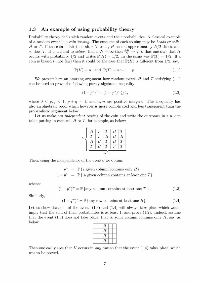
where 0 < p, q < 1, p + q = 1, and n,m are positive integers. This inequality hasalso an algebraic proof which however is more complicated and less transparent than theprobabilistic argument below.Let us make nm independent tossing of the coin and write the outcomes in a n×m

table putting in each cell H or T , for example, as below:

n

⎧⎪⎪⎪⎪⎨⎪⎪⎪⎪⎩H T T H TT T H H HH H T H TT H T T T| z

m

Then, using the independence of the events, we obtain:

pn = P a given column contains only H1− pn = P a given column contains at least one T

whence(1− pn)m = P any column contains at least one T . (1.3)

Similarly,(1− qm)n = P any row contains at least one H . (1.4)

Let us show that one of the events (1.3) and (1.4) will always take place which wouldimply that the sum of their probabilities is at least 1, and prove (1.2). Indeed, assumethat the event (1.3) does not take place, that is, some column contains only H, say, asbelow:

HHHH

Then one easily sees that H occurs in any row so that the event (1.4) takes place, whichwas to be proved.

7

Is this proof rigorous? It may leave impression of a rather empirical argument thana mathematical proof. The point is that we have used in this argument the existence ofevents with certain properties: firstly, H should have probability p where p a given numberin (0, 1) and secondly, there must be enough independent events like that. Certainly,mathematics cannot rely on the existence of biased coins (or even fair coins!) so in orderto make the above argument rigorous, one should have a mathematical notion of eventsand their probabilities, and prove the existence of the events with the required properties.This can and will be done using the measure theory.

1.4 Extension of measure from semi-ring to a ring

Let M be any non-empty set.

Definition. A family S of subsets of M is called a semi-ring if

• S contains ∅

• A,B ∈ S =⇒ A ∩B ∈ S

• A,B ∈ S =⇒ A \B is a disjoint union of a finite family sets from S.

Example. The family of all intervals in R is a semi-ring. Indeed, the intersection oftwo intervals is an interval, and the difference of two intervals is either an interval or thedisjoint union of two intervals. In the same way, the family of all intervals of the form[a, b) is a semi-ring.The family of all rectangles in R2 is also a semi-ring (see Exercise 6).

Definition. A family S if subsets of M is called a ring if

• S contains ∅

• A,B ∈ S =⇒ A ∪B ∈ S and A \B ∈ S.

It follows that also the intersection A ∩B belongs to S because

A ∩B = B \ (B \A)

is also in S. Hence, a ring is closed under taking the set-theoretic operations ∩,∪, \. Also,it follows that a ring is a semi-ring.

Definition. A ring S is called a σ-ring if the union of any countable family Ak∞k=1 ofsets from S is also in S.

It follows that the intersection A =T

kAk is also in S. Indeed, let B be any of thesets Ak so that B ⊃ A. Then

A = B \ (B \A) = B \µS

k

(B \Ak)

¶∈ S.

Trivial examples of rings are S = ∅ , S = ∅,M, or S = 2M — the family of allsubsets of M . On the other hand, the set of the intervals in R is not a ring.

8

Observe that if Sα is a family of rings (σ-rings) then the intersectionT

α Sαis also aring (resp., σ-ring), which trivially follows from the definition.

Definition. Given a family S of subsets of M , denote by R (S) the intersection of allrings containing S.Note that at least one ring containing S always exists: 2M . The ring R (S) is hence

the minimal ring containing S.

Theorem 1.3 Let S be a semi-ring.(a) The minimal ring R (S) consists of all finite disjoint unions of sets from S.(b) If μ is a finitely additive measure on S then μ extends uniquely to a finitely additive

measure on R (S).(c) If μ is a σ-additive measure on S then the extension of μ to R (S) is also σ-additive.

For example, if S is the semi-ring of all intervals on R then the minimal ring R (S)consists of finite disjoint unions of intervals. The notion of the length extends then to allsuch sets and becomes a measure there. Clearly, if a set A ∈ R (S) is a disjoint union ofthe intervals Iknk=1 then (A) =

Pnk=1 (Ik) . This formula follows from the fact that

the extension of to R (S) is a measure. On the other hand, this formula can be used toexplicitly define the extension of .Proof. (a) Let S0 be the family of sets that consists of all finite disjoint unions of sets

from S, that is,

S0 =

½nF

k=1

Ak : Ak ∈ S, n ∈ N¾.

We need to show that S0 = R (S). It suffices to prove that S0 is a ring. Indeed, if we knowthat already then S0 ⊃ R (S) because the ring S0 contains S and R (S) is the minimalring containing S. On the other hand, S0 ⊂ R (S) , because R (S) being a ring containsall finite unions of elements of S and, in particular, all elements of S0.The proof of the fact that S0 is a ring will be split into steps. If A and B are elements

of S then we can write A =Fn

k=1Ak and B =Fm

l=1Bl, where Ak, Bl ∈ S.Step 1. If A,B ∈ S0 and A,B are disjoint then A t B ∈ S0. Indeed, A t B is the

disjoint union of all the sets Ak and Bl so that A tB ∈ S0.Step 2. If A,B ∈ S0 then A ∩B ∈ S0. Indeed, we have

A ∩B =Fk,l

(Ak ∩Bl) .

Since Ak ∩Bl ∈ S by the definition of a semi-ring, we conclude that A ∩B ∈ S0.Step 3. If A,B ∈ S0 then A \B ∈ S0. Indeed, since

A \B =Fk

(Ak \B) ,

it suffices to show that Ak \B ∈ S0 (and then use Step 1). Next, we have

Ak \B = Ak \Fl

Bl =Tl

(Ak \Bl) .

By Step 2, it suffices to prove that Ak\Bl ∈ S0. Indeed, since Ak, Bl ∈ S, by the definitionof a semi-ring we conclude that Ak \Bl is a finite disjoint union of elements of S, whenceAk \Bl ∈ S0.

9

Step 4. If A,B ∈ S0 then A ∪B ∈ S0. Indeed, we have

A ∪B = (A \B)F(B \A)

F(A ∩B) .

By Steps 2 and 3, the sets A \B, B \A, A∩B are in S0, and by Step 1 we conclude thattheir disjoint union is also in S0.By Steps 3 and 4, we conclude that S0 is a ring, which finishes the proof.(b) Now let μ be a finitely additive measure on S. The extension to S0 = R (S) is

unique: if A ∈ R (S) and A =Fn

k=1Ak where Ak ∈ S then necessarily

μ (A) =nX

k=1

μ (Ak) . (1.5)

Now let us prove the existence of μ on S0. For any set A ∈ S0 as above, let us define μ by(1.5) and prove that μ is indeed finitely additive. First of all, let us show that μ (A) doesnot depend on the choice of the splitting of A =

Fnk=1Ak. Let us have another splitting

A =F

lBl where Bl ∈ S. ThenAk =

Fl

Ak ∩Bl

and since Ak ∩Bl ∈ S and μ is finitely additive on S, we obtain

μ (Ak) =Xl

μ (Ak ∩Bl) .

Summing up on k, we obtainXk

μ (Ak) =Xk

Xl

μ (Ak ∩Bl) .

Similarly, we have Xl

μ (Bl) =Xl

Xk

(Ak ∩Bl) ,

whenceP

k μ (Ak) =P

k μ (Bk).Finally, let us prove the finite additivity of the measure (1.5). Let A,B be two disjoint

sets from R (S) and assume that A =F

k Ak and B =F

lBl, where Ak, Bl ∈ S. ThenA tB is the disjoint union of all the sets Ak and Bl whence by the previous argument

μ (A tB) =Xk

μ (Ak) +Xl

μ (Bl) = μ (A) + μ (B) .

If there is a finite family of disjoint sets C1, ..., Cn ∈ R (S) then using the fact that theunions of sets from R (S) is also in R (S), we obtain by induction in n that

μ

µFk

Ck

¶=Xk

μ (Ck) .

(c) Let A =F∞

l=1Bl where A,Bl ∈ R (S). We need to prove that

μ (A) =∞Xl=1

μ (Bl) . (1.6)

10

Represent the given sets in the form A =F

kAk and Bl =F

mBlm where the summationsin k and m are finite and the sets Ak and Blm belong to S. Set also

Cklm = Ak ∩Blm

and observe that Cklm ∈ S. Also, we have

Ak = Ak ∩A = Ak ∩Gl,m

Blm =Gl,m

(Ak ∩Blm) =Gl,m

Cklm

andBlm = Blm ∩A = Blm ∩

Gk

Ak =Gk

(Ak ∩Blm) =Gk

Cklm.

By the σ-additivity of μ on S, we obtain

μ (Ak) =Xl,m

μ (Cklm)

andμ (Blm) =

Xk

μ (Cklm) .

It follows that Xk

μ (Ak) =Xk,l.m

μ (Cklm) =Xl,m

μ (Blm) .

On the other hand, we have by definition of μ on R (S) that

μ (A) =Xk

μ (Ak)

andμ (Bl) =

Xm

μ (Blm)

whence Xl

μ (Bl) =Xl,m

μ (Blm) .

Combining the above lines, we obtain

μ (A) =Xk

μ (Ak) =Xl,m

μ (Blm) =Xl

μ (Bl) ,

which finishes the proof.

1.5 Extension of measure to a σ-algebra

1.5.1 σ-rings and σ-algebras

Recall that a σ-ring is a ring that is closed under taking countable unions (and intersec-tions). For a σ-additive measure, a σ-ring would be a natural domain. Our main aimin this section is to extend a σ-additive measure μ from a ring R to a σ-ring.

11

So far we have only trivial examples of σ-rings: S = ∅ and S = 2M . Implicitexamples of σ-rings can be obtained using the following approach.

Definition. For any family S of subsets of M , denote by Σ (S) the intersection of allσ-rings containing S.

At least one σ-ring containing S exists always: 2M . Clearly, the intersection of anyfamily of σ-rings is again a σ-ring. Hence, Σ (S) is the minimal σ-ring containing S.Most of examples of rings that we have seen so far were not σ-rings. For example, the

ring R that consists of all finite disjoint unions of intervals is not σ-ring because it doesnot contain the countable union of intervals

∞Sk=1

(k, k + 1/2) .

In general, it would be good to have an explicit description of Σ (R), similarly to thedescription of R (S) in Theorem 1.3. One might conjecture that Σ (R) consists of disjointcountable unions of sets from R. However, this is not true. Let R be again the ring offinite disjoint unions of intervals. Consider the following construction of the Cantor setC: it is obtained from [0, 1] by removing the interval

¡13, 23

¢then removing the middle

third of the remaining intervals, etc:

C = [0, 1]\µ1

3,2

3

¶\µ1

9,2

9

¶\µ7

9,8

9

¶\µ1

27,2

27

¶\µ7

27,8

27

¶\µ19

27,20

27

¶\µ25

27,26

27

¶\ ...

Since C is obtained from intervals by using countable union of interval and \, we haveC ∈ Σ (R). However, the Cantor set is uncountable and contains no intervals expect forsingle points (see Exercise 13). Hence, C cannot be represented as a countable union ofintervals.The constructive procedure of obtaining the σ-ring Σ (R) from a ring R is as follows.

Denote by Rσ the family of all countable unions of elements from R. Clearly, R ⊂ Rσ ⊂Σ (R). Then denote by Rσδ the family of all countable intersections from Rσ so that

R ⊂ Rσ ⊂ Rσδ ⊂ Σ (R) .

Define similarly Rσδσ, Rσδσδ, etc. We obtain an increasing sequence of families of sets,all being subfamilies of Σ (R). One might hope that their union is Σ (R) but in generalthis is not true either. In order to exhaust Σ (R) by this procedure, one has to apply ituncountable many times, using the transfinite induction. This is, however, beyond thescope of this course.As a consequence of this discussion, we see that a simple procedure used in Theorem

1.3 for extension of a measure from a semi-ring to a ring, is not going to work in thepresent setting and, hence, the procedure of extension is more complicated.At the first step of extension a measure to a σ-ring, we assume that the full set M is

also an element of R and, hence, μ (M) <∞. Consider the following example: letM be aninterval in R, R consists of all bounded subintervals ofM and μ is the length of an interval.If M is bounded, then M ∈ R. However, if M is unbounded (for example, M = R) thenM does belong to R while M clearly belongs to Σ (R) since M can be represented as acountable union of bounded intervals. It is also clear that for any reasonable extension oflength, μ (M) in this case must be ∞.

12

The assumption M ∈ R and, hence, μ (M) < ∞, simplifies the situation, while theopposite case will be treated later on.

Definition. A ring containing M is called an algebra. A σ-ring in M that contains M iscalled a σ-algebra.

1.5.2 Outer measure

Henceforth, assume that R is an algebra. It follows from the definition of an algebra thatif A ∈ R then Ac := M \ A ∈ R. Also, let μ be a σ-additive measure on R. For any setA ⊂M , define its outer measure μ∗ (A) by

μ∗ (A) = inf

( ∞Xk=1

μ (Ak) : Ak ∈ R and A ⊂∞Sk=1

Al

). (1.7)

In other words, we consider all coverings Ak∞k=1 of A by a sequence of sets from thealgebra R and define μ∗ (A) as the infimum of the sum of all μ (Ak), taken over all suchcoverings.It follows from (1.7) that μ∗ is monotone in the following sense: if A ⊂ B then

μ∗ (A) ≤ μ∗ (B). Indeed, any sequence Ak ⊂ R that covers B, will cover also A, whichimplies that the infimum in (1.7) in the case of the set A is taken over a larger family,than in the case of B, whence μ∗ (A) ≤ μ∗ (B) follows.Let us emphasize that μ∗ (A) is defined on all subsets A ofM , but μ∗ is not necessarily

a measure on 2M . Eventually, we will construct a σ-algebra containing R where μ∗ willbe a σ-additive measure. This will be preceded by a sequence of Lemmas.

Lemma 1.4 For any set A ⊂M , μ∗ (A) <∞. If in addition A ∈ R then μ∗ (A) = μ (A) .

Proof. Note that ∅ ∈ R and μ (∅) = 0 because

μ (∅) = μ (∅ t ∅) = μ (∅) + μ (∅) .

For any set A ⊂ M , consider a covering Ak = M, ∅, ∅, ... of A. Since M, ∅ ∈ R, itfollows from (1.7) that

μ∗ (A) ≤ μ (M) + μ (∅) + μ (∅) + ... = μ (M) <∞.

Assume now A ∈ R. Considering a covering Ak = A, ∅, ∅, ... and using that A, ∅ ∈ R,we obtain in the same way that

μ∗ (A) ≤ μ (A) + μ (∅) + μ (∅) + ... = μ (A) . (1.8)

On the other hand, for any sequence Ak as in (1.7) we have by the σ-subadditivity ofμ (see Exercise 6) that

μ (A) ≤∞Xk=1

μ (Ak) .

Taking inf over all such sequences Ak, we obtain

μ (A) ≤ μ∗ (A) ,

which together with (1.8) yields μ∗ (A) = μ (A).

13

Lemma 1.5 The outer measure μ∗ is σ-subadditive on 2M .

Proof. We need to prove that if

A ⊂∞Sk=1

Ak (1.9)

where A and Ak are subsets of M then

μ∗ (A) ≤∞Xk=1

μ∗ (Ak) . (1.10)

By the definition of μ∗, for any set Ak and for any ε > 0 there exists a sequence Akn∞n=1of sets from R such that

Ak ⊂∞Sn=1

Akn (1.11)

and

μ∗ (Ak) ≥∞Xn=1

μ (Akn)−ε

2k.

Adding up these inequalities for all k, we obtain∞Xk=1

μ∗ (Ak) ≥∞X

k,n=1

μ (Akn)− ε. (1.12)

On the other hand, by (1.9) and (1.11), we obtain that

A ⊂∞S

k,n=1

Akn.

Since Akn ∈ R, we obtain by (1.7)

μ∗ (A) ≤∞X

k,n=1

μ (Akn) .

Comparing with (1.12), we obtain

μ∗ (A) ≤∞Xk=1

μ∗ (Ak) + ε.

Since this inequality is true for any ε > 0, it follows that it is also true for ε = 0, whichfinishes the proof.

1.5.3 Symmetric difference

Definition. The symmetric difference of two sets A,B ⊂M is the set

A M B := (A \B) ∪ (B \A) = (A ∪B) \ (A ∩B) .

Clearly, A M B = B M A. Also, x ∈ A M B if and only if x belongs to exactly one ofthe sets A,B, that is, either x ∈ A and x /∈ B or x /∈ A and x ∈ B.

14

Lemma 1.6 (a) For arbitrary sets A1, A2, B1, B2 ⊂M ,

(A1 A2) M (B1 B2) ⊂ (A1 M B1) ∪ (A2 M B2) , (1.13)

where denotes any of the operations ∪, ∩, \.(b) If μ∗ is an outer measure on M then

|μ∗ (A)− μ∗ (B)| ≤ μ∗ (A M B) , (1.14)

for arbitrary sets A,B ⊂M .

Proof. (a) SetC = (A1 M B1) ∪ (A2 M B2)

and verify (1.13) in the case when is ∪, that is,

(A1 ∪A2) M (B1 ∪B2) ⊂ C. (1.15)

By definition, x ∈ (A1 ∪A2) M (B1 ∪B2) if and only if x ∈ A1 ∪ A2 and x /∈ B1 ∪ B2 orconversely x ∈ B1 ∪B2 and x /∈ A1 ∪A2. Since these two cases are symmetric, it sufficesto consider the first case. Then either x ∈ A1 or x ∈ A2 while x /∈ B1 and x /∈ B2. Ifx ∈ A1 then

x ∈ A1 \B1 ⊂ A1 M B1 ⊂ C

that is, x ∈ C. In the same way one treats the case x ∈ A2, which proves (1.15).For the case when is ∩, we need to prove

(A1 ∩A2) M (B1 ∩B2) ⊂ C. (1.16)

Observe that x ∈ (A1 ∩A2) M (B1 ∩B2) means that x ∈ A1 ∩ A2 and x /∈ B1 ∩ B2or conversely. Again, it suffices to consider the first case. Then x ∈ A1 and x ∈ A2while either x /∈ B1 or x /∈ B2. If x /∈ B1 then x ∈ A1 \ B1 ⊂ C, and if x /∈ B2 thenx ∈ A2 \B2 ⊂ C.For the case when is \, we need to prove

(A1 \A2) M (B1 \B2) ⊂ C. (1.17)

Observe that x ∈ (A1 \A2) M (B1 \B2) means that x ∈ A1 \ A2 and x /∈ B1 \ B2 orconversely. Consider the first case, when x ∈ A1, x /∈ A2 and either x /∈ B1 or x ∈ B2. Ifx /∈ B1 then combining with x ∈ A1 we obtain x ∈ A1 \B1 ⊂ C. If x ∈ B2 then combiningwith x /∈ A2, we obtain

x ∈ B2 \A2 ⊂ A2 M B2 ⊂ C,

which finishes the proof.(b) Note that

A ⊂ B ∪ (A \B) ⊂ B ∪ (A M B)

whence by the subadditivity of μ∗ (Lemma 1.5)

μ∗ (A) ≤ μ∗ (B) + μ∗ (A M B) ,

whenceμ∗ (A)− μ∗ (B) ≤ μ∗ (A M B) .

15

Switching A and B, we obtain a similar estimate

μ∗ (B)− μ∗ (A) ≤ μ∗ (A M B) ,

whence (1.14) follows.

Remark The only property of μ∗ used here was the finite subadditivity. So, inequality(1.14) holds for any finitely subadditive functional.

1.5.4 Measurable sets

We continue considering the case whenR is an algebra onM and μ is a σ-additive measureon R. Recall that the outer measure μ∗ is defined by (1.7).

Definition. A set A ⊂ M is called measurable (with respect to the algebra R and themeasure μ) if, for any ε > 0, there exists B ∈ R such that

μ∗ (A M B) < ε. (1.18)

In other words, set A is measurable if it can be approximated by sets fromR arbitrarilyclosely, in the sense of (1.18).Now we can state one of the main theorems in this course.

Theorem 1.7 (Carathéodory’s extension theorem) Let R be an algebra on a set M andμ be a σ-additive measure on R. Denote byM the family of all measurable subsets of M .Then the following is true.(a) M is a σ-algebra containing R.(b) The restriction of μ∗ onM is a σ-additive measure (that extends measure μ from

R toM).(c) If eμ is a σ-additive measure defined on a σ-algebra Σ such that

R ⊂ Σ ⊂M,

then eμ = μ∗ on Σ.

Hence, parts (a) and (b) of this theorem ensure that a σ-additive measure μ canbe extended from the algebra R to the σ-algebra of all measurable sets M. Moreover,applying (c) with Σ =M, we see that this extension is unique.Since the minimal σ-algebra Σ (R) is contained inM, it follows that measure μ can

be extended from R to Σ (R). Applying (c) with Σ = Σ (R), we obtain that this extensionis also unique.Proof. We split the proof into a series of claims.

Claim 1 The familyM of all measurable sets is an algebra containing R.If A ∈ R then A is measurable because

μ∗ (A M A) = μ∗ (∅) = μ (∅) = 0

where μ∗ (∅) = μ (∅) by Lemma 1.4. Hence, R ⊂M. In particular, also the entire spaceM is a measurable set.

16

In order to verify thatM is an algebra, it suffices to show that if A1, A2 ∈M thenalso A1∪A2 and A1\A2 are measurable. Let us prove this for A = A1∪A2. By definition,for any ε > 0 there are sets B1, B2 ∈ R such that

μ∗ (A1 M B1) < ε and μ∗ (A2 M B2) < ε. (1.19)

Setting B = B1 ∪B2 ∈ R, we obtain by Lemma 1.6,

A M B ⊂ (A1 M B1) ∪ (A2 M B2)

and by the subadditivity of μ∗ (Lemma 1.5)

μ∗ (A M B) ≤ μ∗ (A1 M B1) + μ∗ (A2 M B2) < 2ε. (1.20)

Since ε > 0 is arbitrary andB ∈ R we obtain that A satisfies the definition of a measurableset.The fact that A1 \A2 ∈M is proved in the same way.

Claim 2 μ∗ is σ-additive onM.SinceM is an algebra and μ∗ is σ-subadditive by Lemma 1.5, it suffices to prove that

μ∗ is finitely additive onM (see Exercise 9).Let us prove that, for any two disjoint measurable sets A1 and A2, we have

μ∗ (A) = μ∗ (A1) + μ∗ (A2)

where A = A1FA2. By Lemma 1.5, we have the inequality

μ∗ (A) ≤ μ∗ (A1) + μ∗ (A2)

so that we are left to prove the opposite inequality

μ∗ (A) ≥ μ∗ (A1) + μ∗ (A2) .

As in the previous step, for any ε > 0 there are sets B1, B2 ∈ R such that (1.19) holds.Set B = B1 ∪B2 ∈ R and apply Lemma 1.6, which says that

|μ∗ (A)− μ∗ (B)| ≤ μ∗ (A M B) < 2ε,

where in the last inequality we have used (1.20). In particular, we have

μ∗ (A) ≥ μ∗ (B)− 2ε. (1.21)

On the other hand, since B ∈ R, we have by Lemma 1.4 and the additivity of μ on R,that

μ∗ (B) = μ (B) = μ (B1 ∪B2) = μ (B1) + μ (B2)− μ (B1 ∩B2) . (1.22)

Next, we will estimate here μ (Bi) from below via μ∗ (Ai), and show that μ (B1 ∩B2) issmall enough. Indeed, using (1.19) and Lemma 1.6, we obtain, for any i = 1, 2,

|μ∗ (Ai)− μ∗ (Bi)| ≤ μ∗ (Ai M Bi) < ε

whenceμ (B1) ≥ μ∗ (A1)− ε and μ (B2) ≥ μ∗ (A2)− ε. (1.23)

17

On the other hand, by Lemma 1.6 and using A1 ∩A2 = ∅, we obtain

B1 ∩B2 = (A1 ∩A2) M (B1 ∩B2) ⊂ (A1 M B1) ∪ (A2 M B2)

whence by (1.20)

μ (B1 ∩B2) = μ∗ (B1 ∩B2) ≤ μ∗ (A1 M B1) + μ∗ (A2 M B2) < 2ε. (1.24)

It follows from (1.21)—(1.24) that

μ∗ (A) ≥ (μ∗ (A1)− ε) + (μ∗ (A2)− ε)− 2ε− 2ε = μ∗ (A1) + μ∗ (A2)− 6ε.

Letting ε→ 0, we finish the proof.

Claim 3M is σ-algebra.Assume that An∞n=1 is a sequence of measurable sets and prove that A :=

S∞n=1An

is also measurable. Note that

A = A1 ∪ (A2 \A1) ∪ (A3 \A2 \A1) ... =∞Fn=1

eAn,

where eAn := An \An−1 \ ... \A1 ∈M

(here we use the fact that M is an algebra — see Claim 1). Therefore, renaming eAn toAn, we see that it suffices to treat the case of a disjoint union: given A =

F∞n=1An where

An ∈M, prove that A ∈M.Note that, for any fixed N ,

μ∗ (A) ≥ μ∗µ

NFn=1

An

¶=

NXn=1

μ∗ (An) ,

where we have used the monotonicity of μ∗ and the additivity of μ∗ on M (Claim 2).This implies by N →∞ that

∞Xn=1

μ∗ (An) ≤ μ∗ (A) <∞

(cf. Lemma 1.4), so that the seriesP∞

n=1 μ∗ (An) converges. In particular, for any ε > 0,

there is N ∈ N such that∞X

n=N+1

μ∗ (An) < ε.

Setting

A0 =NFn=1

An and A00 =∞F

n=N+1

An,

we obtain by the σ-subadditivity of μ∗

μ∗ (A00) ≤∞X

n=N+1

μ∗ (An) < ε.

18

By Claim 1, the set A0 is measurable as a finite union of measurable sets. Hence, there isB ∈ R such that

μ∗ (A0 M B) < ε.

Since A = A0 ∪A00, we have

A M B ⊂ (A0 M B) ∪A00. (1.25)

Indeed, x ∈ A M B means that x ∈ A and x /∈ B or x /∈ A and x ∈ B. In the first case,we have x ∈ A0 or x ∈ A00. If x ∈ A0 then together with x /∈ B it gives

x ∈ A0 M B ⊂ (A0 M B) ∪A00.

If x ∈ A00 then the inclusion is obvious. In the second case, we have x /∈ A0 which togetherwith x ∈ B implies x ∈ A0 M B, which finishes the proof of (1.25).It follows from (1.25) that

μ∗ (A M B) ≤ μ∗ (A0 M B) + μ∗ (A00) < 2ε.

Since ε > 0 is arbitrary and B ∈ R, we conclude that A ∈M.Claim 4 Let Σ be a σ-algebra such that

R ⊂ Σ ⊂M

and let eμ be a σ-additive measure on Σ such that eμ = μ on R. Then eμ = μ∗ on Σ.We need to prove that eμ (A) = μ∗ (A) for any A ∈ Σ By the definition of μ∗, we have

μ∗ (A) = inf

( ∞Xn=1

μ (An) : An ∈ R and A ⊂∞Sn=1

An

).

Applying the σ-subadditivity of eμ (see Exercise 7), we obtaineμ (A) ≤ ∞X

n=1

eμ (An) =∞Xn=1

μ (An) .

Taking inf over all such sequences An, we obtaineμ (A) ≤ μ∗ (A) . (1.26)

On the other hand, since A is measurable, for any ε > 0 there is B ∈ R such that

μ∗ (A M B) < ε. (1.27)

By Lemma 1.6(b),|μ∗ (A)− μ∗ (B)| ≤ μ∗ (A M B) < ε. (1.28)

Note that the proof of Lemma 1.6(b) uses only subadditivity of μ∗. Since eμ is alsosubadditive, we obtain that

|eμ (A)− eμ (B)| ≤ eμ (A M B) ≤ μ∗ (A M B) < ε,

where we have also used (1.26) and (1.27) . Combining with (1.28) and using eμ (B) =μ (B) = μ∗ (B), we obtain

|eμ (A)− μ∗ (A)| ≤ |μ∗ (A)− μ∗ (B)|+ |eμ (A)− eμ (B)| < 2ε.Letting ε→ 0, we conclude that eμ (A) = μ∗ (A) ,which finishes the proof.

19

1.6 σ-finite measures

Recall Theorem 1.7: any σ-additive measure on an algebra R can be uniquely extendedto the σ-algebra of all measurable sets (and to the minimal σ-algebra containing R).Theorem 1.7 has a certain restriction for applications: it requires that the full set M

belongs to the initial ring R (so that R is an algebra). For example, if M = R and R isthe ring of the bounded intervals then this condition is not satisfied. Moreover, for anyreasonable extension of the notion of length, the length of the entire line R must be ∞.This suggest that we should extended the notion of a measure to include also the valuesof ∞.So far, we have not yet defined the term “measure” itself using “finitely additive

measures” and “σ-additive measures”. Now we define the notion of a measure as follows.

Definition. Let M be a non-empty set and S be a family of subsets of M . A functionalμ : S → [0,+∞] is called a measure if, for all sets A,Ak ∈ S such that A =

FNk=1Ak

(where N is either finite or infinite), we have

μ (A) =NXk=1

μ (Ak) .

Hence, a measure is always σ-additive. The difference with the previous definition of“σ-additive measure” is that we allow for measure to take value +∞. In the summation,we use the convention that (+∞) + x = +∞ for any x ∈ [0,+∞].Example. Let S be the family of all intervals on R (including the unbounded intervals)and define the length of any interval I ⊂ R with the endpoints a, b by (I) = |b− a|where a and b may take values from [−∞,+∞]. Clearly, for any unbounded interval Iwe have (I) = +∞. We claim that is a measure on S in the above sense.Indeed, let I =

FNk=1 Ik where I, Ik ∈ S and N is either finite or infinite. We need to

prove that

(I) =NXk=1

(Ik) (1.29)

If I is bounded then all intervals Ik are bounded, and (1.29) follows from Theorem 1.1. Ifone of the intervals Ik is unbounded then also I is unbounded, and (1.29) is true becausethe both sides are +∞. Finally, consider the case when I is unbounded while all Ikare bounded. Choose any bounded closed interval I 0 ⊂ I. Since I 0 ⊂

S∞k=1 Ik, by the

σ-subadditivity of the length on the ring of bounded intervals (Lemma 1.2), we obtain

(I 0) ≤NXk=1

(Ik) .

By the choose of I 0, the length (I 0) can be made arbitrarily large, whence it follows that

NXk=1

(Ik) = +∞ = (I) .

20

Of course, allowing the value+∞ for measures, we receive trivial examples of measuresas follows: just set μ (A) = +∞ for any A ⊂M . The following definition is to ensure theexistence of plenty of sets with finite measures.

Definition. A measure μ on a set S is called finite ifM ∈ S and μ (M) <∞. A measureμ is called σ-finite if there is a sequence Bk∞k=1 of sets from S such that μ (Bk) < ∞and M =

S∞k=1Bk.

Of course, any finite measure is σ-finite. The measure in the setting of Theorem 1.7is finite. The length defined on the family of all intervals in R, is σ-finite but not finite.Let R be a ring in a set M . Our next goal is to extend a σ-finite measure μ from R

to a σ-algebra. For any B ∈ R, define the family RB of subsets of B by

RB = R ∩ 2B = A ⊂ B : A ∈ R .

Observe that RB is an algebra in B (indeed, RB is a ring as the intersection of two rings,and also B ∈ RB). If μ (B) <∞ then μ is a finite measure on RB and by Theorem 1.7,μ extends uniquely to a finite measure μB on the σ-algebraMB of measurable subsets ofB. Our purpose now is to construct a σ-algebraM of measurable sets in M and extendmeasure μ to a measure onM.Let Bk∞k=1 be a sequence of sets from R such that M =

S∞k=1Bk and μ (Bk) < ∞

(such sequence exists by the σ-finiteness of μ). Replacing the sets Bk by the differences

B1, B2 \B1, B3 \B1 \B2, ...,

we can assume that all Bk are disjoint, that is, M =F∞

k=1Bk. In what follows, we fixsuch a sequence Bk.Definition. A set A ∈ M is called measurable if A ∩ Bk ∈ MBk

for any k. For anymeasurable set A, set

μM (A) =Xk

μBk(A ∩Bk) . (1.30)

Theorem 1.8 Let μ be a σ-finite measure on a ring R andM be the family of all mea-surable sets defined above. Then the following is true.(a)M is a σ-algebra containing R.(b) The functional μM defined by (1.30) is a measure on M that extends measure μ

on R.(c) If eμ is a measure defined on a σ-algebra Σ such that

R ⊂ Σ ⊂M,

then eμ = μM on Σ.

Proof. (a) If A ∈ R then A ∩ Bk ∈ R because Bk ∈ R. Therefore, A ∩ Bk ∈ RBk

whence A ∩Bk ∈MBkand A ∈M. Hence, R ⊂M.

Let us show that if A =SN

n=1An where An ∈M then also A ∈M (where N can be∞). Indeed, we have

A ∩Bk =Sn

(An ∩Bk) ∈MBk

21

because An ∩ Bk ∈MBkandMBk

is a σ-algebra. Therefore, A ∈M. In the same way,if A0, A00 ∈M then the difference A = A0 \A00 belongs toM because

A ∩Bk = (A0 ∩Bk) \ (A00 ∩Bk) ∈MBk

.

Finally, M ∈M becauseM ∩Bk = Bk ∈MBk

.

Hence,M satisfies the definition of a σ-algebra.(b) If A ∈ R then A ∩Bk ∈ RBk

whence μBk(A ∩Bk) = μ (A ∩Bk) . Since

A =Fk

(A ∩Bk) ,

and μ is a measure on R, we obtain

μ (A) =Xk

μ (A ∩Bk) =Xk

μBk(A ∩Bk) .

Comparing with (1.30), we obtain μM (A) = μ (A). Hence, μM on R coincides with μ.Let us show that μM is a measure. Let A =

FNn=1An where An ∈M and N is either

finite or infinite. We need to prove that

μM (A) =Xn

μM (An) .

Indeed, we have Xn

μM (An) =Xn

Xk

μBk(An ∩Bk)

=Xk

Xn

μBk(An ∩Bk)

=Xk

μBk

µFn

(An ∩Bk)

¶=

Xk

μBk(A ∩Bk)

= μM (A) ,

where we have used the fact that

A ∩Bk =Fn

(An ∩Bk)

and the σ-additivity of measure μBk.

(c) Let eμ be another measure defined on a σ-algebra Σ such that R ⊂ Σ ⊂M andeμ = μ on R. Let us prove that eμ (A) = μM (A) for any A ∈ Σ. Observing that eμ and μcoincide on RBk

, we obtain by Theorem 1.7 that eμ and μBkcoincide on ΣBk

:= Σ ∩ 2Bk .Then for any A ∈ Σ, we have A =

Fk (A ∩Bk) and A ∩Bk ∈ ΣBk

whenceeμ (A) =Xk

eμ (A ∩Bk) =Xk

μBk(A ∩Bk) =

Xk

μM (A) ,

which finishes the proof.

Remark. The definition of a measurable set uses the decomposition M =F

kBk whereBk are sets from R with finite measure. It seems to depend on the choice of Bk but infact it does not. Here is an equivalent definition: a set A ⊂ M is called measurable ifA ∩B ∈ RB for any B ∈ R. For the proof see Exercise 19.

22

1.7 Null sets

Let R be a ring on a set M and μ be a finite measure on R (that is, μ is a σ-additivefunctional on R and μ (M) <∞). Let μ∗ be the outer measure as defined by (1.7).Definition. A set A ⊂ M is called a null set (or a set of measure 0) if μ∗ (A) = 0. Thefamily of all null sets is denoted by N .Using the definition (1.7) of the outer measure, one can restate the condition μ∗ (A) = 0

as follows: for any ε > 0 there exists a sequence Ak∞k=1 ⊂ R such that

A ⊂Sk

Ak andXk

μ (Ak) < ε.

If the ring R is the minimal ring containing a semi-ring S (that is, R = R (S)) then thesequence Ak in the above definition can be taken from S. Indeed, if Ak ⊂ R then, byTheorem 1.3, Ak is a disjoint finite union of some sets Akn from S where n varies in afinite set. It follows that

μ (Ak) =Xn

μ (Akn)

and Xk

μ (Ak) =Xk

Xn

μ (Akn) .

Since the double sequence Akn covers A, the sequence Ak ⊂ R can be replaced bythe double sequence Akn ⊂ S.

Example. Let S be the semi-ring of intervals in R and μ be the length. It is easy tosee that a single point set x is a null set. Indeed, for any ε > 0 there is an interval Icovering x and such that (I) < ε. Moreover, we claim that any countable set A ⊂ R isa null set. Indeed, if A = xk∞k=1 then cover xk by an interval Ik of length < ε

2kso that

the sequence Ik of intervals covers A andP

k (Ik) < ε. Hence, A is a null set. Forexample, the set Q of all rationals is a null set. The Cantor set from Exercise 13 is anexample of an uncountable set of measure 0.In the same way, any countable subset of R2 is a null set (with respect to the area).

Lemma 1.9 (a) Any subset of a null set is a null set.(b) The family N of all null sets is a σ-ring.(c) Any null set is measurable, that is, N ⊂M.

Proof. (a) It follows from the monotonicity of μ∗ that B ⊂ A implies μ∗ (B) ≤ μ∗ (A).Hence, if μ∗ (A) = 0 then also μ∗ (B) = 0.(b) If A,B ∈ N then A \ B ∈ N by part (a), because A \ B ⊂ A. Let A =

SNn=1An

where An ∈ N and N is finite or infinite. Then, by the σ-subadditivity of μ∗ (Lemma1.5), we have

μ∗ (A) ≤Xn

μ∗ (An) = 0

whence A ∈ N .(c) We need to show that if A ∈ N then, for any ε > 0 there is B ∈ R such that

μ∗ (A M B) < ε. Indeed, just take B = ∅ ∈ R. Then μ∗ (A M B) = μ∗ (A) = 0 < ε, whichwas to be proved.

23

Let now μ be a σ-finite measure on a ring R. Then we have M =F∞

k=1Bk whereBk ∈ R and μ (Bk) <∞.Definition. In the case of a σ-finite measure, a set A ⊂M is called a null set if A ∩Bk

is a null set in each Bk.Lemma 1.9 easily extends to σ-finite measures: one has just to apply the corresponding

part of Lemma 1.9 to each Bk.Let Σ = Σ (R) be the minimal σ-algebra containing a ring R so that

R ⊂ Σ ⊂M.

The relation between two σ-algebras Σ andM is given by the following theorem.

Theorem 1.10 Let μ be a σ-finite measure on a ring R. Then A ∈ M if and only ifthere is B ∈ Σ such that A M B ∈ N , that is, μ∗ (A M B) = 0.

This can be equivalently stated as follows:

— A ∈M if and only if there is B ∈ Σ and N ∈ N such that A = B M N .

— A ∈M if and only if there is N ∈ N such that A M N ∈ Σ.

Indeed, Theorem 1.10 says that for any A ∈M there is B ∈ Σ and N ∈ N such thatA M B = N . By the properties of the symmetric difference, the latter is equivalent toeach of the following identities: A = B M N and B = A M N (see Exercise 15), whichsettle the claim.Proof of Theorem 1.10. We prove the statement in the case when measure μ is

finite. The case of a σ-finite measure follows then straightforwardly.By the definition of a measurable set, for any n ∈ N there is Bn ∈ R such that

μ∗ (A M Bn) < 2−n.

The set B ∈ Σ, which is to be found, will be constructed as a sort of limit of Bn asn→∞. For that, set

Cn = Bn ∪Bn+1 ∪ ... =∞Sk=n

Bk

so that Cn∞n=1 is a decreasing sequence, and define B by

B =∞Tn=1

Cn.

Clearly, B ∈ Σ since B is obtain from Bn ∈ R by countable unions and intersections. Letus show that

μ∗ (A M B) = 0.

We haveA M Cn = A M

∞Sk=n

Bk ⊂∞Sk=n

(A M Bk)

(see Exercise 15) whence by the σ-subadditivity of μ∗ (Lemma 1.5)

μ∗ (A M Cn) ≤∞Xk=n

μ∗ (A M Bk) <∞Xk=n

2−k = 21−n.

24

Since the sequence Cn∞n=1 is decreasing, the intersection of all sets Cn does not changeif we omit finitely many terms. Hence, we have for any N ∈ N

B =∞T

n=N

Cn.

Hence, using again Exercise 15, we have

A M B = A M∞T

n=N

Cn ⊂∞S

n=N

(A M Cn)

whence

μ∗ (A M B) ≤∞X

n=N

μ∗ (A M Cn) ≤∞X

n=N

21−n = 22−N .

Since N is arbitrary here, letting N →∞ we obtain μ∗ (A M B) = 0.Conversely, let us show that if A M B is null set for some B ∈ Σ then A is measurable.

Indeed, the set N = A M B is a null set and, by Lemma 1.9, is measurable. SinceA = B M N and both B and N are measurable, we conclude that A is also measurable.

1.8 Lebesgue measure in Rn

Now we apply the above theory of extension of measures to Rn. For that, we need thenotion of the product measure.

1.8.1 Product measure

Let M1 and M2 be two non-empty sets, and S1, S2 be families of subsets of M1 and M2,respectively. Consider the set

M =M1 ×M2 := (x, y) : x ∈M1, y ∈M2and the family S of subsets of M , defined

S = S1 × S2 := A×B : A ∈ S1, B ∈ S2 .

For example, if M1 =M2 = R then M = R2. If S1 and S2 are families of all intervalsin R then S consists of all rectangles in R2.Claim. If S1 and S2 are semi-rings then S is also a semi-ring (see Exercise 6).In the sequel, let S1 and S2 be semi-rings.Let μ1 be a finitely additive measure on the semi-ring S1 and μ2 be a finitely additive

measure on the semi-ring S2. Define the product measure μ = μ1 × μ2 on S as follows: ifA ∈ S1 and B ∈ S2 then set

μ (A×B) = μ1 (A)μ2 (B) .

Claim. μ is also a finitely additive measure on S (see By Exercise 20).

Remark. It is true that if μ1 and μ2 are σ-additive then μ is σ-additive as well, but theproof in the full generality is rather hard and will be given later in the course.By induction, one defines the product of n semi-rings and the product of n measures

for any n ∈ N.

25

1.8.2 Construction of measure in Rn.

Let S1 be the semi-ring of all bounded intervals in R and define Sn (being the family ofsubsets of Rn = R× ...×R) as the product of n copies of S1:

Sn = S1 × S1 × ...× S1.

That is, any set A ∈ Sn has the form

A = I1 × I2 × ...× In (1.31)

where Ik are bounded intervals in R. In other words, Sn consists of bounded boxes.Clearly, Sn is a semi-ring as the product of semi-rings. Define the product measure λn onSn by

λn = × ...×where is the length on S1. That is, for the set A from (1.31),

λn (A) = (I1) .... (In) .

Then λn is a finitely additive measure on the semi-ring Sn in Rn.

Lemma 1.11 λn is a σ-additive measure on Sn.

Proof. We use the same approach as in the proof of σ-additivity of (Theorem 1.1),which was based on the finite additivity of and on the compactness of a closed boundedinterval. Since λn is finitely additive, in order to prove that it is also σ-additive, it sufficesto prove that λn is regular in the following sense: for any A ∈ Sn and any ε > 0, thereexist a closed box K ∈ Sn and an open box U ∈ Sn such that

K ⊂ A ⊂ U and λn (U) ≤ λn (K) + ε

(see Exercise 17). Indeed, if A is as in (1.31) then, for any δ > 0 and for any index j,there is a closed interval Kj and an open interval Uj such that

Kj ⊂ Ij ⊂ Uj and (Uj) ≤ (Kj) + δ.

Set K = K1 × ...×Kn and U = U1 × ...× Un so that K is closed, U is open, and

K ⊂ A ⊂ U.

It also follows that

λn (U) = (U1) ... (Un) ≤ ( (K1) + δ) ... ( (Kn) + δ) < (K1) ... (Kn) + ε = λn (K) + ε,

provided δ = δ (ε) is chosen small enough. Hence, λn is regular, which finishes the proof.

Note that measure λn is also σ-finite. Indeed, let us cover R by a sequence Ik∞k=1 ofbounded intervals. Then all possible products Ik1 × Ik2 × ...× Ikn forms a covering of Rn

by a sequence of bounded boxes. Hence, λn is a σ-finite measure on Sn.By Theorem 1.3, λn can be uniquely extended as a σ-additive measure to the minimal

ring Rn = R (Sn), which consists of finite union of bounded boxes. Denote this extension

26

also by λn. Then λn is a σ-finite measure on Rn. By Theorem 1.8, λn extends uniquely tothe σ-algebraMn of all measurable sets in Rn. Denote this extension also by λn. Hence,λn is a measure on the σ-algebraMn that contains Rn.

Definition. Measure λn onMn is called the Lebesgue measure in Rn. The measurablesets in Rn are also called Lebesgue measurable.

In particular, the measure λ2 in R2 is called area and the measure λ3 in R3 is calledvolume. Also, λn for any n ≥ 1 is frequently referred to as an n-dimensional volume.

Definition. The minimal σ-algebra Σ (Rn) containing Rn is called the Borel σ-algebraand is denoted by Bn (or by B (Rn)). The sets from Bn are called the Borel sets (or Borelmeasurable sets).

Hence, we have the inclusions Sn ⊂ Rn ⊂ Bn ⊂Mn.

Example. Let us show that any open subset U of Rn is a Borel set. Indeed, for any x ∈ Uthere is an open box Bx such that x ∈ Bx ⊂ U . Clearly, Bx ∈ Rn and U =

Sx∈U Bx.

However, this does not immediately imply that U is Borel since the union is uncountable.To fix this, observe that Bx can be chosen so that all the coordinates of Bx (that is, allthe endpoints of the intervals forming Bx) are rationals. The family of all possible boxesin Rn with rational coordinates is countable. For every such box, we can see if it occurs inthe family Bxx∈U or not. Taking only those boxes that occur in this family, we obtainan at most countable family of boxes, whose union is also U . It follows that U is a Borelset as a countable union of Borel sets.Since closed sets are complements of open sets, it follows that also closed sets are Borel

sets. Then we obtain that countable intersections of open sets and countable unions ofclosed sets are also Borel, etc. Any set, that can be obtained from open and closed setsby applying countably many unions, intersections, subtractions, is again a Borel set.

Example. Any non-empty open set U has a positive Lebesgue measure, because Ucontains a non-empty box B and λ (B) > 0. As an example, let us show that thehyperplane A = xn = 0 of Rn has measure 0. It suffices to prove that the intersectionA ∩B is a null set for any bounded box B in Rn. Indeed, set

B0 = A ∩B = x ∈ B : xn = 0

and note that B0 is a bounded box in Rn−1. Choose ε > 0 and set

Bε = B0 × (−ε, ε) = x ∈ B : |xn| < ε

so that Bε is a box in Rn and B0 ⊂ Bε. Clearly,

λn (Bε) = λn−1 (B0) (−ε, ε) = 2ελn−1 (B0) .

Since ε can be made arbitrarily small, we conclude that B0 is a null set.

Remark. Recall that Bn ⊂Mn and, by Theorem 1.10, any set fromMn is the symmetricdifference of a set from Bn and a null set. An interesting question is whether the familyMn of Lebesgue measurable sets is actually larger than the family Bn of Borel sets. Theanswer is yes. Although it is difficult to construct an explicit example of a set inMn \Bn

27

the fact thatMn \ Bn is non-empty can be used comparing the cardinal numbers |Mn|and |Bn|. Indeed, it is possible to show that

|Bn| = |R| <¯2R¯= |Mn| , (1.32)

which of course implies thatMn \Bn is non-empty. Let us explain (not prove) why (1.32)is true. As we have seen, any open set is the union of a countable sequence of boxeswith rational coordinates. Since the cardinality of such sequences is |R|, it follows thatthe family of all open sets has the cardinality |R|. Then the cardinality of the countableintersections of open sets amounts to that of countable sequences of reals, which is again|R| . Continuing this way and using the transfinite induction, one can show that thecardinality of the family of the Borel sets is |R|.To show that |Mn| =

¯2R¯, we use the fact that any subset of a null set is also a null

set and, hence, is measurable. Assume first that n ≥ 2 and let A be a hyperplane fromthe previous example. Since |A| = |R| and any subset of A belongs to Mn, we obtainthat |Mn| ≥

¯2A¯=¯2R¯, which finishes the proof. If n = 1 then the example with a

hyperplane does not work, but one can choose A to be the Cantor set (see Exercise 13),which has the cardinality |R| and measure 0. Then the same argument works.

1.9 Probability spaces

Probability theory can be considered as a branch of a measure theory where one usesspecific notation and terminology, and considers specific questions. We start with theprobabilistic notation and terminology.

Definition. A probability space is a triple (Ω,F ,P) where

• Ω is a non-empty set, which is called the sample space.

• F is a σ-algebra of subsets of Ω, whose elements are called events.

• P is a probability measure on F , that is, P is a measure on F and P (Ω) = 1 (inparticular, P is a finite measure). For any event A ∈ F , P(A) is called the probabilityof A.

Since F is an algebra, that is, Ω ∈ F , the operation of taking complement is definedin F , that is, if A ∈ F then the complement Ac := Ω \ A is also in F . The event Ac isopposite to A and

P (Ac) = P (Ω \A) = P (Ω)− P (A) = 1− P (A) .

Example. 1. Let Ω = 1, 2, ..., N be a finite set, and F is the set of all subsets of Ω.Given N non-negative numbers pi such that

PNi=1 pi = 1, define P by

P(A) =Xi∈A

pi. (1.33)

The condition (1.33) ensures that P (Ω) = 1.

28

For example, in the simplest case N = 2, F consists of the sets ∅, 1 , 2 , 1, 2.Given two non-negative numbers p and q such that p+q = 1, set P (1) = p, P (2) = q,while P (∅) = 0 and P (1, 2) = 1.This example can be generalized to the case when Ω is a countable set, say, Ω = N.

Given a sequence pi∞i=1 of non-negative numbers pi such thatP∞

i=1 pi = 1, define for anyset A ⊂ Ω its probability by (1.33). Measure P constructed by means of (1.33) is calleda discrete probability measure, and the corresponding space (Ω,F ,P) is called a discreteprobability space.

2. Let Ω = [0, 1], F be the set of all Lebesgue measurable subsets of [0, 1] and P bethe Lebesgue measure λ1 restricted to [0, 1]. Clearly, (Ω,F ,P) is a probability space.

1.10 Independence

Let (Ω,F ,P) be a probability space.Definition. Two events A and B are called independent (unabhängig) if

P(A ∩B) = P(A)P(B).

More generally, let Ai be a family of events parametrized by an index i. Then thefamily Ai is called independent (or one says that the events Ai are independent) if, forany finite set of distinct indices i1, i2, ..., ik,

P(Ai1 ∩Ai2 ∩ ... ∩Aik) = P(Ai1)P(Ai2)...P(Aik). (1.34)

For example, three events A,B,C are independent if

P (A ∩B) = P (A)P (B) , P (A ∩ C) = P (A)P (C) , P (B ∩ C) = P (B)P (C)P (A ∩B ∩ C) = P (A)P (B)P (C) .

Example. In any probability space (Ω,F ,P), any couple A,Ω is independent, for anyevent A ∈ F , which follows from

P(A ∩ Ω) = P(A) = P(A)P(Ω).

Similarly, the couple A, ∅ is independent. If the couple A,A is independent then P(A) = 0or 1, which follows from

P(A) = P(A ∩A) = P(A)2.

Example. Let Ω be a unit square [0, 1]2, F consist of all measurable sets in Ω andP = λ2. Let I and J be two intervals in [0, 1], and consider the events A = I × [0, 1] andB = [0, 1]× J . We claim that the events A and B are independent. Indeed, A∩B is therectangle I × J , and

P(A ∩B) = λ2(I × J) = (I) (J) .

SinceP(A) = (I) and P(B) = (J) ,

29

we concludeP(A ∩B) = P(A)P(B).

We may choose I and J with the lengths p and q, respectively, for any prescribed couplep, q ∈ (0, 1). Hence, this example shows how to construct two independent event withgiven probabilities p, q.In the same way, one can construct n independent events (with prescribed probabili-

ties) in the probability space Ω = [0, 1]n where F is the family of all measurable sets inΩ and P is the n-dimensional Lebesgue measure λn. Indeed, let I1, ..., In be intervals in[0, 1] of the length p1, ..., pn. Consider the events

Ak = [0, 1]× ...× Ik × ...× [0, 1] ,

where all terms in the direct product are [0, 1] except for the k-th term Ik. Then Ak is abox in Rn and

P (Ak) = λn (Ak) = (Ik) = pk.

For any sequence of distinct indices i1, i2, ..., ik, the intersection

Ai1 ∩Ai2 ∩ ... ∩Aik

is a direct product of some intervals [0, 1] with the intervals Ii1, ..., Iik so that

P (Ai1 ∩ ... ∩Aik) = pi1...pik = P (Ai1) ...P (Ain) .

Hence, the sequence Aknk=1 is independent.It is natural to expect that independence is preserved by certain operations on events.

For example, let A,B,C,D be independent events and let us ask whether the followingcouples of events are independent:

1. A ∩B and C ∩D

2. A ∪B and C ∪D

3. E = (A ∩B) ∪ (C \A) and D.

It is easy to show that A ∩B and C ∩D are independent:

P ((A ∩B) ∩ (C ∩D)) = P (A ∩B ∩ C ∩D)= P(A)P(B)P(C)P(D) = P(A ∩B)P(C ∩D).

It is less obvious how to prove that A ∪ B and C ∪D are independent. This will followfrom the following more general statement.

Lemma 1.12 Let A = Ai be an independent family of events. Suppose that a familyA0 of events is obtained from A by one of the following procedures:

1. Adding to A one of the events ∅ or Ω.

2. Replacing two events A,B ∈ A by one event A ∩B,

3. Replacing an event A ∈ A by its complement Ac.

30

4. Replacing two events A,B ∈ A by one event A ∪B.

5. Replacing two events A,B ∈ A by one event A \B.

Then the family A0 is independent.

Applying the operation 4 twice, we obtain that if A,B,C,D are independent thenA∪B and C ∪D are independent. However, this lemma still does not answer why E andD are independent.Proof. Each of the above procedures removes from A some of the events and adds

a new event, say N . Denote by A00 the family that remains after the removal, so thatA0 is obtained from A00 by adding N . Clearly, removing events does not change theindependence, so that A00 is independent. Hence, in order to prove that A0 is independent,it suffices to show that, for any events A1, A2, ..., Ak from A00 with distinct indices,

P(N ∩A1 ∩ ... ∩Ak) = P(N)P(A1)...P(Ak). (1.35)

Case 1. N = ∅ or Ω. The both sides of (1.35) vanish if N = ∅. If N = Ω thenit can be removed from both sides of (1.35), so (1.35) follows from the independence ofA1, A2, ..., Ak.Case 2. N = A ∩B. We have

P((A ∩B) ∩A1 ∩A2 ∩ ... ∩Ak) = P(A)P(B)P(A1)P(A2)...P(Ak)

= P(A ∩B)P(A1)P(A2)...P(Ak),

which proves (1.35).Case 3. N = Ac. Using the identity

Ac ∩B = B \A = B \ (A ∩B)

and its consequenceP (Ac ∩B) = P (A)− P (A ∩B) ,

we obtain, for B = A1 ∩A2 ∩ ... ∩Ak, that

P(Ac ∩A1 ∩A2 ∩ ... ∩Ak) = P(A1 ∩A2 ∩ ... ∩Ak)− P(A ∩A1 ∩A2 ∩ ... ∩Ak)

= P(A1)P(A2)...P(Ak)− P(A)P(A1)P(A2)...P(Ak)

= (1− P(A))P(A1)P(A2)...P(Ak)

= P(Ac)P(A1)P(A2)...P(Ak)

Case 4. N = A ∪B. By the identity

A ∪B = (Ac ∩Bc)c

this case amounts to 2 and 3.Case 5. N = A \B. By the identity

A \B = A ∩Bc

this case amounts to 2 and 3.

31

Example. Using Lemma 1.12, we can justify the probabilistic argument, introduced inSection 1.3 in order to prove the inequality

(1− pn)m + (1− qm)n ≥ 1, (1.36)

where p, q ∈ [0, 1], p+ q = 1, and n,m ∈ N. Indeed, for that argument we need nm inde-pendent events, each with the given probability p. As we have seen in an example above,there exists an arbitrarily long finite sequence of independent events, and with arbitrarilyprescribed probabilities. So, choose nm independent events each with probability p anddenote them by Aij where i = 1, 2, ..., n and j = 1, 2, ...,m, so that they can be arrangedin a n×m matrix Aij . For any index j (which is a column index), consider an event

Cj =nTi=1

Aij,

that is, the intersection of all events Aij in the column j. Since Aij are independent, weobtain

P(Cj) = pn and P(Ccj ) = 1− pn.

By Lemma 1.12, the events Cj are independent and, hence, Ccj are also independent.

Setting

C =mTj=1

Ccj

we obtainP(C) = (1− pn)m.

Similarly, considering the events

Ri =mTj=1

Acij

andR =

nTi=1

Rci ,

we obtain in the same way that

P(R) = (1− qm)n.

Finally, we claim thatC ∪R = Ω, (1.37)

which would imply thatP (C) + P (R) ≥ 1,

that is, (1.36).To prove (1.37), observe that, by the definitions of R and C,

C =mTj=1

Ccj =

mTj=1

µnTi=1

Aij

¶c

=mTj=1

nSi=1

Acij

and

Rc =

µnTi=1

Rci

¶c

=nSi=1

Ri =nSi=1

mTj=1

Acij.

32

Denoting by ω an arbitrary element of Ω, we see that if ω ∈ Rc then there is an indexi0 such that ω ∈ Ac

i0jfor all j. This implies that ω ∈

Sni=1A

cij for any j, whence ω ∈ C.

Hence, Rc ⊂ C, which is equivalent to (1.37).Let us give an alternative proof of (1.37) which is a rigorous version of the argument

with the coin tossing. The result of nm trials with coin tossing was a sequence of lettersH,T (heads and tails). Now we make a sequence of digits 1, 0 instead as follows: for anyω ∈ Ω, set

Mij (ω) =

½1, ω ∈ Aij,0, ω /∈ Aij.

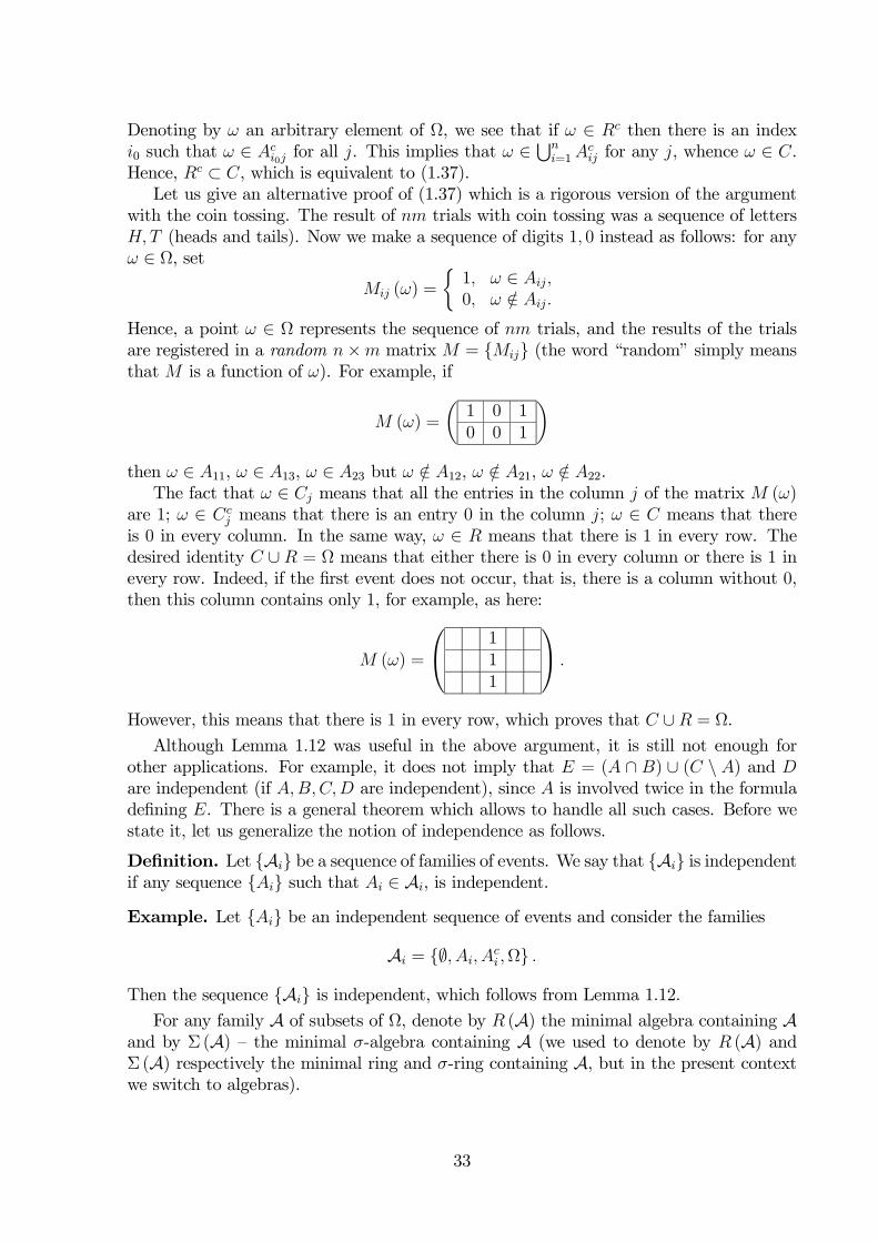
Hence, a point ω ∈ Ω represents the sequence of nm trials, and the results of the trialsare registered in a random n×m matrix M = Mij (the word “random” simply meansthat M is a function of ω). For example, if

M (ω) =

µ1 0 10 0 1

¶then ω ∈ A11, ω ∈ A13, ω ∈ A23 but ω /∈ A12, ω /∈ A21, ω /∈ A22.The fact that ω ∈ Cj means that all the entries in the column j of the matrix M (ω)

are 1; ω ∈ Ccj means that there is an entry 0 in the column j; ω ∈ C means that there

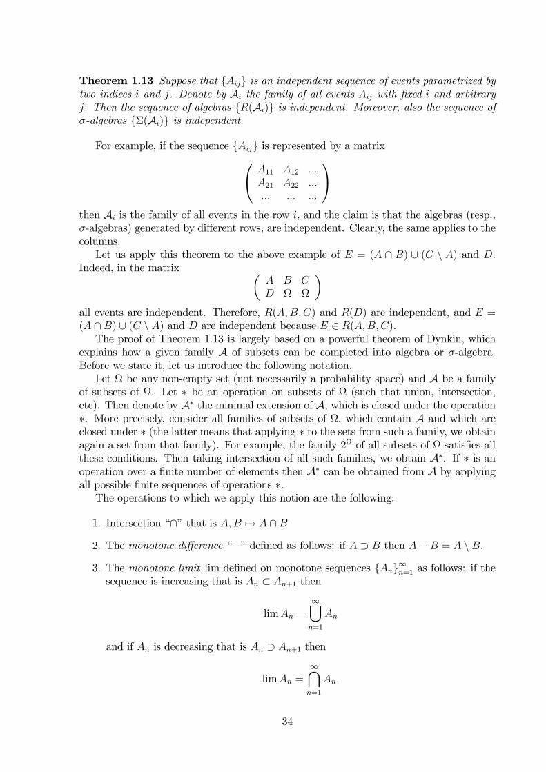
is 0 in every column. In the same way, ω ∈ R means that there is 1 in every row. Thedesired identity C ∪ R = Ω means that either there is 0 in every column or there is 1 inevery row. Indeed, if the first event does not occur, that is, there is a column without 0,then this column contains only 1, for example, as here:

M (ω) =

⎛⎝ 111

⎞⎠ .

However, this means that there is 1 in every row, which proves that C ∪R = Ω.

Although Lemma 1.12 was useful in the above argument, it is still not enough forother applications. For example, it does not imply that E = (A ∩ B) ∪ (C \ A) and Dare independent (if A,B,C,D are independent), since A is involved twice in the formuladefining E. There is a general theorem which allows to handle all such cases. Before westate it, let us generalize the notion of independence as follows.

Definition. Let Ai be a sequence of families of events. We say that Ai is independentif any sequence Ai such that Ai ∈ Ai, is independent.

Example. Let Ai be an independent sequence of events and consider the families

Ai = ∅, Ai, Aci ,Ω .

Then the sequence Ai is independent, which follows from Lemma 1.12.

For any family A of subsets of Ω, denote by R (A) the minimal algebra containing Aand by Σ (A) — the minimal σ-algebra containing A (we used to denote by R (A) andΣ (A) respectively the minimal ring and σ-ring containing A, but in the present contextwe switch to algebras).

33

Theorem 1.13 Suppose that Aij is an independent sequence of events parametrized bytwo indices i and j. Denote by Ai the family of all events Aij with fixed i and arbitraryj. Then the sequence of algebras R(Ai) is independent. Moreover, also the sequence ofσ-algebras Σ(Ai) is independent.

For example, if the sequence Aij is represented by a matrix⎛⎝ A11 A12 ...A21 A22 ...... ... ...

⎞⎠then Ai is the family of all events in the row i, and the claim is that the algebras (resp.,σ-algebras) generated by different rows, are independent. Clearly, the same applies to thecolumns.Let us apply this theorem to the above example of E = (A ∩ B) ∪ (C \ A) and D.

Indeed, in the matrix µA B CD Ω Ω

¶all events are independent. Therefore, R(A,B,C) and R(D) are independent, and E =(A ∩B) ∪ (C \A) and D are independent because E ∈ R(A,B,C).The proof of Theorem 1.13 is largely based on a powerful theorem of Dynkin, which

explains how a given family A of subsets can be completed into algebra or σ-algebra.Before we state it, let us introduce the following notation.Let Ω be any non-empty set (not necessarily a probability space) and A be a family

of subsets of Ω. Let ∗ be an operation on subsets of Ω (such that union, intersection,etc). Then denote by A∗ the minimal extension of A, which is closed under the operation∗. More precisely, consider all families of subsets of Ω, which contain A and which areclosed under ∗ (the latter means that applying ∗ to the sets from such a family, we obtainagain a set from that family). For example, the family 2Ω of all subsets of Ω satisfies allthese conditions. Then taking intersection of all such families, we obtain A∗. If ∗ is anoperation over a finite number of elements then A∗ can be obtained from A by applyingall possible finite sequences of operations ∗.The operations to which we apply this notion are the following:

1. Intersection “∩” that is A,B 7→ A ∩B

2. The monotone difference “−” defined as follows: if A ⊃ B then A−B = A \B.

3. The monotone limit lim defined on monotone sequences An∞n=1 as follows: if thesequence is increasing that is An ⊂ An+1 then

limAn =∞[n=1

An

and if An is decreasing that is An ⊃ An+1 then

limAn =∞\n=1

An.

34

Using the above notation, A− is the minimal extension of A using the monotonedifference, and Alim is the minimal extension of A using the monotone limit.

Theorem 1.14 (Theorem of Dynkin) Let Ω be an arbitrary non-empty set and A be afamily of subsets of Ω.

(a) If A contains Ω and is closed under ∩ then

R(A) = A−.

(b) If A is algebra of subsets of Ω then

Σ(A) = Alim.

As a consequence we see that if A is any family of subsets containing Ω then it canbe extended to the minimal algebra R (A) as follows: firstly, extend it using intersectionsso that the resulting family A∩ is closed under intersections; secondly, extend A∩ tothe algebra R (A∩) = R (A) using the monotone difference (which requires part (a) ofTheorem 1.14). Hence, we obtain the identity

R(A) = (A∩)− . (1.38)

Similarly, applying further part (b), we obtain

Σ(A) =³(A∩)−

´lim. (1.39)

The most non-trivial part is (1.38). Indeed, it says that any set that can be obtainedfrom sets of A by a finite number of operations ∩,∪, \, can also be obtained by firstapplying a finite number of ∩ and then applying finite number of “−”. This is not quiteobvious even for the simplest case

A = Ω, A,B .

Indeed, (1.38) implies that the union A ∪ B can be obtained from Ω, A,B by applyingfirst ∩ and then “−”. However, Theorem 1.14 does not say how exactly one can do that.The answer in this particular case is

A ∪B = Ω− (Ω−A− (B − (A ∩B))).

Proof of Theorem 1.14. Let us prove the first part of the theorem. Assuming thatA contains Ω and is closed under ∩, let us show that A− is algebra, which will settle theclaim. Indeed, as an algebra, A− must contain R(A) since R (A) is the smallest algebraextension of A. On the other hand, R(A) is closed under “−” and contains A; then itcontains also A−, whence R(A) = A−.To show that A− is an algebra, we need to verify that A− contains ∅,Ω and is closed

under ∩,∪, \. Obviously, Ω ∈ A− and ∅ = Ω − Ω ∈ A−. Also, if A ∈ A− then alsoAc ∈ Ac because Ac = Ω− A. It remains to show that A− is closed under intersections,that is, if A,B ∈ A− then A∩B ∈ A− (this will imply that also A∪B = (Ac ∩Bc)c ∈ A−and A \B = A− (A ∩B) ∈ A−).

35

Given a set A ∈ A−, call a set B ⊂ Ω suitable for A if A∩B ∈ A−. Denote the familyof suitable sets by S, that is,

S =©B ⊂ Ω : A ∩B ∈ A−

ª.

We need to prove that S ⊃ A−. Assume first that A ∈ A. Then S contains A becauseA is closed under intersections. Let us verify that S is closed under monotone difference.Indeed, if B1 ⊃ B2 are suitable sets then

A ∩ (B1 −B2) = (A ∩B1)− (A ∩B2) ∈ A−,

whence B1 ∩ B2 ∈ S. Hence, the family S of all suitable sets contains A and is closedunder “−”, which implies that S contains A− (because A− is the minimal family withthese properties). Hence, we have proved that

A ∩B ∈ A− (1.40)

whenever A ∈ A and B ∈ A−. Switching A and B, we see that (1.40) holds also if A ∈ A−and B ∈ A.Now we prove (1.40) for all A,B ∈ A−. Consider again the family S of suitable sets

for A. As we have just shown, S ⊃ A. Since S is closed under “−”, we conclude thatS ⊃ A−, which finishes the proof.The second statement about σ-algebras can be obtained similarly. Using the method

of suitable sets, one proves that Alim is an algebra, and the rest follows from the followingobservation.

Lemma 1.15 If an algebra A is closed under monotone limits then it is a σ-algebra(conversely, any σ-algebra is an algebra and is closed under lim).

Indeed, it suffices to prove that if An ∈ A for all n ∈ N thenS∞

n=1An ∈ A. Indeed,setting Bn =

Sni=1Ai, we have the identity

∞[n=1

An =∞[n=1

Bn = limBn.

Since Bn ∈ A, it follows that also limBn ∈ A, which finishes the proof.Theorem 1.13 will be deduced from the following more general theorem.

Theorem 1.16 Let (Ω,F ,P) be a probability space. Let Ai be a sequence of familiesof events such that each family Ai contain Ω and is closed under ∩. If the sequence Aiis independent then the sequence of the algebras R(Ai) is also independent. Moreover,the sequence of σ-algebras Σ(Ai) is independent, too.

Proof of Theorem 1.16. In order to check the independence of families, one needsto test finite sequences of events chosen from those families. Hence, it suffice to restrict tothe case when the number of families Ai is finite. So, assume that i runs over 1, 2, ..., n.It suffices to show that the sequence R(A1),A2, ...,An is independent. If we know thatthen we can by induction replace A2 by R(A2) etc. To show the independence of this

36

sequence, we need to take arbitrary events A1 ∈ R(A1), A2 ∈ A2, ..., An ∈ An and provethat

P(A1 ∩A2 ∩ ... ∩An) = P(A1)P(A2)...P(An). (1.41)

Indeed, by the definition of the independent events, one needs to check this property alsofor subsequences Aik but this amounts to the full sequence Ai by setting the missingevents to be Ω.Denote for simplicity A = A1 and B = A2 ∩ A3 ∩ ... ∩ An. Since A2, A3, ..., An are

independent, (1.41) amounts to

P(A ∩B) = P(A)P(B). (1.42)

In other words, we are left to prove that A and B are independent, for any A ∈ R(A1)and B being an intersection of events from A2,A3, ...,An.Fix such B and call an event A suitable for B if (1.42) holds. We need to show that

all events from R(A1) are suitable. Observe that all events from A1 are suitable. Letus prove that the family of suitable sets is closed under the monotone difference “−”.Indeed, if A and A0 are suitable and A ⊃ A0 then

P((A−A0) ∩B) = P(A ∩B)− P(A0 ∩B)= P(A)P(B)− P(A0)P(B)= P(A−A0)P(B).

Hence, we conclude that the family of all suitable sets contains the extension of A1 by“−”, that is A−1 . By Theorem 1.14, A−1 = R(A1). Hence, all events from R(A1) aresuitable, which was to be proved.The independence of Σ(Ai) is treated in the same way by verifying that the equality

(1.42) is preserved by monotone limits.Proof of Theorem 1.13. Adding to each family Ai the event Ω does not change

the independence, so we may assume Ω ∈ Ai. Also, if we extend Ai to A∩i then A∩i are also independent. Indeed, each event Bi ∈ A∩i is an intersection of a finite number ofevents from Ai, that is, has the form

Bi = Aij1 ∩Aij2 ∩ ... ∩Aijk .

Hence, the sequence Bi can be obtained by replacing in the double sequence Aijsome elements by their intersections (and throwing away the rest), and the independenceof Bi follows by Lemma 1.12 from the independence of Aij across all i and j.Therefore, the sequence A∩i satisfies the hypotheses of Theorem 1.16, and the se-

quence R(A∩i ) (and Σ(A∩i )) is independent. Since R(A∩i ) = R(Ai) and Σ(A∩i ) =Σ(Ai), we obtain the claim.

37

2 Integration

In this Chapter, we define the general notion of the Lebesgue integral. Given a set M , aσ-algebraM and a measure μ onM, we should be able to define the integralZ

M

f dμ

of any function f on M of an appropriate class. Recall that if M is a bounded closedinterval [a, b] ⊂ R then the integral

R baf (x) dx is defined for Riemann integrable function,

in particular, for continuous functions on [a, b], and is obtained as the limit of the Riemannintegral sums

nXi=1

f (ξi) (xi − xi−1)

where xini=0 is a partition of the interval [a, b] and ξini=1 is a sequence of tags, that is,

ξi ∈ [xi−1, xi]. One can try also in the general case arrange a partition of the set M intosmaller sets E1, E2,... and define the integral sumsX

i

f (ξi)μ (Ei)

where ξi ∈ Ei. There are two problems here: in what sense to understand the limit ofthe integral sums and how to describe the class of functions for which the limit exists.Clearly, the partition Ei should be chosen so that the values of f in Ei do not changemuch and can be approximated by f (ξi). In the case of the Riemann integrals, this isachieved by choosing Ei to be small intervals and by using the continuity of f . In thegeneral case, there is another approach, due to Lebesgue, whose main idea is to chooseEi depending of f , as follows:

Ei = x ∈M : ci−1 < f (x) ≤ ci

where ci is an increasing sequence of reals. The values of f inEi are all inside the interval(ci−1, ci] so that they are all close to f (ξi) provided the sequence ci is fine enough. Thischoice of Ei allows to avoid the use of the continuity of f but raised another question: inorder to use μ (Ei), sets Ei must lie in the domain of the measure μ. For this reason, itis important to have measure defined on possibly larger domain. On the other hand, wewill have to restrict functions f to those for which the sets of the form a < f (x) ≤ bare in the domain of μ. Functions with this property are called measurable. So, we firstgive a precise definition and discuss the properties of measurable functions.

2.1 Measurable functions

Let M be an arbitrary non-empty set andM be a σ-algebra of subsets of M .

Definition. We say that a set A ⊂ M is measurable if A ∈M. We say that a functionf : M → R is measurable if, for any c ∈ R, the set x ∈M : f (x) ≤ c is measurable,that is, belongs toM.

Of course, the measurability of sets and functions depends on the choice of the σ-algebraM. For example, in Rn we distinguish Lebesgue measurable sets and functions

38

whenM =Mn (they are frequently called simply “measurable”), and the Borel measur-able sets and functions whenM = Bn (they are normally called “Borel sets” and “Borelfunctions” avoiding the word “measurable”).The measurability of a function f can be also restated as follows. Since

f (x) ≤ c = f−1(−∞, c],

we can say that a function f is measurable if, for any c ∈ R, the set f−1(−∞, c] ismeasurable. Let us refer to the intervals of the form (−∞, c] as special intervals. Then wecan say that a mapping f : M → R is measurable if the preimage of any special intervalis a measurable set.

Example. Let A be an arbitrary subset ofM . Define the indicator function 1A onM by

1A (x) =

½1, x ∈ A,0, x /∈ A.

We claim that the set A is measurable if and only if the function 1A is measurable. Indeed,the set f (x) ≤ c can be described as follows:

f (x) ≤ c =

⎧⎨⎩ ∅, c < 0,Ac, 0 ≤ c < 1,M, c ≥ 1.

The sets ∅ and M are always measurable, and Ac is measurable if and only if A ismeasurable, whence the claim follows.

Example. Let M = Rn andM = Bn. Let f (x) be a continuous function from Rn to R.Then the set f−1(−∞, c] is a closed subset of Rn as the preimage of a closed set (−∞, c]in R. Since the closed sets are Borel, we conclude that any continuous function f is aBorel function.

Definition. A mapping f : M → Rn is called measurable if, for all c1, c2, ..., cn ∈ R, theset

x ∈M : f1 (x) ≤ c1, f2 (x) ≤ c2, ..., fn (x) ≤ cnis measurable. Here fk is the k-th component of f .In other words, consider an infinite box in Rn of the form:

B = (−∞, c1]× (−∞, c2]× ...× (−∞, cn],

and call it a special box. Then a mapping f : M → Rn is measurable if, for any specialbox B, the preimage f−1 (B) is a measurable subset of M .

Lemma 2.1 If a mapping f : M → Rn is measurable then, for any Borel set A ⊂ Rn,the preimage f−1 (A) is a measurable set.

Proof. Let A be the family of all sets A ⊂ Rn such that f−1 (A) is measurable. Byhypothesis, A contains all special boxes. Let us prove that A is a σ-algebra (this followsalso from Exercise 4 since in the notation of that exercise A = f (M)). If A,B ∈ A thenf−1(A) and f−1(B) are measurable whence

f−1(A \B) = f−1(A) \ f−1(B) ∈M,

39

whence A \B ∈ A. Also, if AkNk=1 is a finite or countable sequence of sets from A thenf−1 (Ak) is measurable for all k whence

f−1µ

NSk=1

Ak

¶=

NSk=1

f−1 (Ak) ∈M,

which implies thatSN

k=1Ak ∈ A. Finally, A contains R because R is the countable unionof the intervals (−∞, n] where n ∈ N, and A contains ∅ = R \R.Hence, A is a σ-algebra containing all special boxes. It remains to show that A

contains all the boxes in Rn, which will imply that A contains all Borel sets in Rn. Infact, it suffices to show that any box in Rn can be obtained from special boxes by acountable sequence of set-theoretic operations.Assume first n = 1 and consider different types of intervals. If A = (−∞, a] then

A ∈ A by hypothesis.Let A = (a, b] where a < b. Then A = (−∞, b]\ (−∞, a], which proves that A belongs

to A as the difference of two special intervals.Let A = (a, b) where a < b and a, b ∈ R. Consider a strictly increasing sequence

bk∞k=1 such that bk → b as k → ∞. Then the intervals (a, bk] belong to A by theprevious argument, and the obvious identity

A = (a, b) =∞Sk=1

(a, bk]

implies that A ∈ A.Let A = [a, b). Consider a strictly increasing sequence ak∞k=1 such that ak → a as

k →∞. Then (ak, b) ∈ A by the previous argument, and the set

A = [a, b) =∞Tk=1

(ak, b)

is also in A.Finally, let A = [a, b]. Observing that A = R \ (−∞, a) \ (b,+∞) where all the terms

belong to A, we conclude that A ∈ A.Consider now that general case n > 1. We are given that A contains all boxes of the

formB = I1 × I2 × ...× In

where Ik are special intervals, and we need to prove that A contains all boxes of this formwith arbitrary intervals Ik. If I1 is an arbitrary interval and I2, ..., In are special intervalsthen one shows that B ∈A using the same argument as in the case n = 1 since I1 can beobtained from the special intervals by a countable sequence of set-theoretic operations,and the same sequence of operations can be applied to the product I1× I2× ...× In. Nowlet I1 and I2 be arbitrary intervals and I3, ..., In be special. We know that if I2 is specialthen B ∈ A. Obtaining an arbitrary interval I2 from special intervals by a countablesequence of operations, we obtain that B ∈ A also for arbitrary I1 and I2. Continuingthe same way, we obtain that B ∈ A if I1, I2, I3 are arbitrary intervals while I4, ..., In arespecial, etc. Finally, we allow all the intervals I1, ..., In to be arbitrary.

Example. If f :M → R is a measurable function then the set

x ∈M : f (x) is irrational

40

is measurable, because this set coincides with f−1(Qc), and Qc is Borel since Q is Borelas a countable set.

Theorem 2.2 Let f1, ..., fn be measurable functions from M to R and let Φ be a Borelfunction from Rn to R. Then the function

F = Φ (f1, ..., fn)

is measurable.

In other words, the composition of a Borel function with measurable functions is mea-surable. Note that the composition of two measurable functions may be not measurable.

Example. It follows from Theorem 2.2 that if f1 and f2 are two measurable functions onM then their sum f1 + f2 is also measurable. Indeed, consider the function Φ (x1, x2) =x1+x2 in R2, which is continuous and, hence, is Borel. Then f1+f2 = Φ (f1, f2) and thisfunction is measurable by Theorem 2.2. A direct proof by definition may be difficult: thefact that the set f1 + f2 ≤ c is measurable, is not immediately clear how to reduce thisset to the measurable sets f1 ≤ a and f1 ≤ b .In the same way, the functions f1f2, f1/f2 (provided f2 6= 0) are measurable. Also,

the functions max (f1, f2) and min (f1, f2) are measurable, etc.

Proof of Theorem 2.2. Consider the mapping f :M → Rn whose components arefk. This mapping is measurable because for any c ∈ Rn, the set

x ∈M : f1 (x) ≤ c1, ..., fn (x) ≤ cn = f1 (x) ≤ c1 ∩ f2 (x) ≤ c2 ∩ ... ∩ fn (x) ≤ cn

is measurable as the intersection of measurable sets. Let us show that F−1 (I) is a mea-surable set for any special interval I, which will prove that F is measurable. Indeed, sinceF (x) = Φ (f (x)), we obtain that

F−1 (I) = x ∈M : F (x) ∈ I= x ∈M : Φ (f (x)) ∈ I=

©x ∈M : f (x) ∈ Φ−1 (I)

ª= f−1

¡Φ−1 (I)

¢.

Since Φ−1 (I) is a Borel set, we obtain by Lemma 2.1 that f−1 (Φ−1 (I)) is measurable,which proves that F−1 (I) is measurable.

Example. If A1, A2, ..., An is a finite sequence of measurable sets then the function

f = c11A1 + c11A2 + ...+ cn1An

is measurable (where ci are constants). Indeed, each of the function 1Ai is measurable,whence the claim following upon application of Theorem 2.2 with the function

Φ (x) = c1x1 + ...+ cnxn.

41

2.2 Sequences of measurable functions

As before, let M be a non-empty set andM be a σ-algebra on M .

Definition. We say that a sequence fn∞n=1 of functions on M converges to a functionf pointwise and write fn → f if fn (x)→ f (x) as n→∞ for any x ∈M .

Theorem 2.3 Let fn∞n=1 be a sequence of measurable functions that converges pointwiseto a function f . Then f is measurable, too.

Proof. Fix some real c. Using the definition of a limit and the hypothesis thatfn (x) → f (x) as n → ∞, we obtain that the inequality f (x) ≤ c is equivalent to thefollowing condition: for any k ∈ N there is m ∈ N such that, for all n ≥ m,

fn (x) < c+1

k.

This can be written in the form of set-theoretic inclusion as follows:

f (x) ≤ c =∞Tk=1

∞Sm=1

∞Tn=m

½fn (x) < c+

1

k

¾.

(Indeed, any logical condition “for any ...” transforms to the intersection of the corre-sponding sets, and the condition “there is ...” transforms to the union.)Since the set fn < c+ 1/k is measurable and the measurability is preserved by

countable unions and intersections, we conclude that the set f (x) ≤ c is measurable,which finishes the proof.

Corollary. Let fn∞n=1 be a sequence of Lebesgue measurable (or Borel) functions on Rn

that converges pointwise to a function f . Then f is Lebesgue measurable (resp., Borel) aswell.

Proof. Indeed, this is a particular case of Theorem 2.3 withM =Mn (for Lebesguemeasurable functions) and withM = Bn (for Borel functions).Example. Let us give an alternative proof of the fact that any continuous function f onR is Borel. Indeed, consider first a function of the form

g (x) =∞Xk=1

ck1Ik (x)

where Ik is a disjoint sequence of intervals. Then

g (x) = limN→∞

NXk=1

ck1Ik (x)

and, hence, g (x) is Borel as the limit of Borel functions. Now fix some n ∈ N and considerthe following sequence of intervals:

Ik = [k

n,k + 1

n) where k ∈ Z,

42

so that R =F

k∈Z Ik. Also, consider the function

gn (x) =Xk∈Z

f

µk

n

¶1Ik (x) .

By the continuity of f , for any x ∈ R, we have gn (x) → f (x) as n → ∞. Hence, weconclude that f is Borel as the pointwise limit of Borel functions.

So far we have only assumed thatM is a σ-algebra of subsets ofM . Now assume thatthere is also a measure μ onM.

Definition. We say that a measure μ is complete if any subset of a set of measure 0belongs toM. That is, if A ∈M and μ (A) = 0 then every subset A0 of A is also inM(and, hence, μ (A0) = 0).

As we know, if μ is a σ-finite measure initially defined on some ring R then by theCarathéodory extension theorems (Theorems 1.7 and 1.8), μ can be extended to a measureon a σ-algebra M of measurable sets, which contains all null sets. It follows that ifμ (A) = 0 then A is a null set and, by Theorem 1.10, any subset of A is also a nullset and, hence, is measurable. Therefore, any measure μ that is constructed by theCarathéodory extension theorems, is automatically compete. In particular, the Lebesguemeasure λn with the domainMn is complete.In general, a measure does not have to be complete, It is possible to show that the

Lebesgue measure λn restricted to Bn is no longer complete (this means, that ifA is aBorel set of measure 0 in Rn then not necessarily any subset of it is Borel). On theother hand, every measure can be completed by adding to its domain the null sets — seeExercise 36.Assume in the sequence that μ is a complete measure defined on a σ-algebra M of

subsets of M . Then we use the term a null set as synonymous for a set of measure 0.

Definition. We say that two functions f, g : M → R are equal almost everywhere andwrite f = g a.e. if the set x ∈M : f (x) 6= g (x) has measure 0. In other words, there isa set N of measure 0 such that f = g on M \N .More generally, the term “almost everywhere” is used to indicate that some property

holds for all points x ∈M \N where μ (N) = 0.

Claim 1. The relation f = g a.e.is an equivalence relation.Proof. We need to prove three properties that characterize the equivalence relations:

1. f = f a.e.. Indeed, the set f (x) 6= f (x) is empty and, hence, is a null set.

2. f = g a.e.is equivalent to g = f a.e., which is obvious.

3. f = g a.e.and g = h a.e. imply f = h a.e. Indeed, we have

f 6= h ⊂ f 6= g ∪ h 6= g

whence we conclude that the set f (x) 6= g (x) is a null set as a subset of the unionof two null sets.

Claim 2 If f is measurable and g = f a.e. then g is also measurable.

43

Proof. Fix some real c and prove that the set g ≤ c is measurable. Observe that

N := f ≤ c M g ≤ c ⊂ f 6= g .

Indeed, x ∈ N if x belongs to exactly to one of the sets f ≤ c and g ≤ c. Forexample, x belongs to the first one and does not belong to the second one, then f (x) ≤ cand g (x) > c whence f (x) 6= g (x). Since f 6= g is a null set, the set N is also a nullset. Then we have

g ≤ c = f ≤ c M N,

which implies that g ≤ c is measurable.Definition. We say that a sequence of functions fn on M converges to a function falmost everywhere and write fn → f a.e. if the set x ∈M : fn (x) 6→ f (x) is a null set.In other words, there is a set N of measure 0 such that fn → f pointwise on M \N .

Theorem 2.4 If fn is a sequence of measurable functions and fn → f a.e. then f isalso a measurable function.

Proof. Consider the set

N = x ∈M : fn (x) 6→ f (x) ,

which has measure 0. Redefine fn (x) for x ∈ N by setting fn (x) = 0. Since we havechanged fn on a null set, the new function fn is also measurable. Then the new sequencefn (x) converges for all x ∈M , because fn (x)→ f (x) for all x ∈M \N by hypothesis,and fn (x) → 0 for all x ∈ N by construction. By Theorem 2.3, the limit functionis measurable, and since f is equal to the limit function almost everywhere, f is alsomeasurable.We say a sequence of functions fn on a set M converges to a function f uniformly

on M and write fn ⇒ f on M if

supx∈M

|fn (x)− f (x)|→ 0 as n→∞.

We have obviously the following relations between the convergences:

f ⇒ f =⇒ fn → f pointwise =⇒ fn → f a.e. (2.1)

In general the converse for the both implications is not true. For example, let us showthat the pointwise convergence does not imply the uniform convergence if the set M isinfinite. Indeed, let xk∞k=1 be a sequence of distinct points in M and set fk = 1xk.Then, for any point x ∈M , fk (x) = 0 for large enough k, which implies that fk (x)→ 0pointwise. On the other hand, sup |fk| = 1 so that fk 6⇒ 0.For the second example, let fk be any sequence of functions that converges pointwise

to f . Define ef as an arbitrary modification of f on a non-empty set of measure 0. Thenstill f → ef a.e. while f does not converge to ef pointwise.Surprisingly enough, the convergence a.e. still implies the uniform convergence but on

a smaller set, as is stated in the following theorem.

44

Theorem 2.5 (Theorem of Egorov) Let μ be a complete finite measure on a σ-algebraM on a set M . Let fn be a sequence of measurable functions and assume that fn → fa.e. on M . Then, for any ε > 0, there is a set Mε ⊂M such that:

1. μ (M \Mε) < ε

2. fn ⇒ f on Mε.

In other words, by removing a set M \Mε is measure smaller than ε, one can achievethat on the remaining set Mε the convergence is uniform.Proof. The condition fn ⇒ f on Mε (where Mε is yet to be defined) means that for

any m ∈ N there is n = n (m) such that for all k ≥ n

supMε

|fk − f | < 1

m.

Hence, for any x ∈Mε,

for any m ≥ 1 for any k ≥ n (m) |fk (x)− f (x)| < 1

m,

which implies that

Mε ⊂∞T

m=1

Tk≥n(m)

½x ∈M : |fk (x)− f (x)| < 1

m

¾.

Now we can defineMε to be the right hand side of this relation, but first we need to definen (m).For any couple of positive integers n,m, consider the set

Am,n =

½x ∈M : |fk (x)− f (x)| < 1

mfor all k ≥ n

¾.

This can also be written in the form

Am,n =Tk≥n

½x ∈M : |fk (x)− f (x)| < 1

m

¾.

By Theorem 2.4, function f is measurable, by Theorem 2.2 the function |fn − f | is mea-surable, which implies that Amn is measurable as a countable intersection of measurablesets.Observe that, for any fixed m, the set Am,n increases with n. Set

Am =∞Sn=1

Am,n = limn→∞

Am,n,

that is, Am is the monotone limit of Am,n. Then, by Exercise 9, we have

μ (Am) = limn→∞

μ (Am,n)

whencelimn→∞

μ (Am \Am,n) = 0 (2.2)

45

(to pass to (2.2), we use that μ (Am) <∞, which is true by the hypothesis of the finitenessof measure μ).Claim For any m, we have

μ (M \Am) = 0. (2.3)

Indeed, by definition,

Am =∞Sn=1

Am,n =∞Sn=1

Tk≥n

½x ∈M : |fk (x)− f (x)| < 1

m

¾,

which means that x ∈ Am if and only if there is n such that for all k ≥ n,

|fk (x)− f (x)| < 1

m.

In particular, if fk (x) → f (x) for some point x then this condition is satisfied so thatthis point x is in Am. By hypothesis, fn (x)→ f (x) for almost all x, which implies thatμ (M \Am) = 0.It follows from (2.2) and (2.3) that

limn→∞

μ (M \Am,n) = 0,

which implies that there is n = n (m) such that

μ¡M \Am,n(m)

¢<

ε

2m. (2.4)

Set

Mε =∞T

m=1

Am,n(m) =∞T

m=1

Tk≥n(m)

½x ∈M : |fk (x)− f (x)| < 1

m

¾(2.5)

and show that the set Mε satisfies the required conditions.1. Proof of μ (M \Mε) < ε. Observe that by (2.5)

μ (M \Mε) = μ

µµ ∞Tm=1

Am,n(m)

¶c¶= μ

µ ∞Sm=1

Acn,m(n)

¶≤

∞Xm=1

μ¡M \An,m(n)

¢<

∞Xm=1

ε

2m= ε.

Here we have used the subadditivity of measure and (2.4).2. Proof of fn ⇒ f on Mε. Indeed, for any x ∈ M , we have by (2.5) that, for any

m ≥ 1 and any k ≥ n (m),

|fk (x)− f (x)| < 1

m.

Hence, taking sup in x ∈Mε, we obtain that also

supMε

|fk − f | ≤ 1

m,

which implies thatsupMε

|fk − f |→ 0

and, hence, fk ⇒ f on Mε.

46

2.3 The Lebesgue integral for finite measures

Let M be an arbitrary set, M be a σ-algebra on M and μ be a complete measure onM. We are going to define the notion of the integral

RMfdμ for an appropriate class of

functions f . We will first do this for a finite measure, that is, assuming that μ (M) <∞,and then extend to the σ-finite measure.Hence, assume here that μ is finite.

2.3.1 Simple functions

Definition. A function f : M → R is called simple if it is measurable and the set of itsvalues is at most countable.

Let ak be the sequence of distinct values of a simple function f . Consider the sets

Ak = x ∈M : f (x) = ak (2.6)

which are measurable, and observe that

M =Fk

Ak. (2.7)

Clearly, we have the identityf (x) =

Xk

ak1Ak (x) (2.8)

for all x ∈ M . Note that any sequence Ak of disjoint measurable sets such that (2.7)and any sequence of distinct reals ak determine by (2.8) a function f (x) that satisfiesalso (2.6), which means that all simple functions have the form (2.8).

Definition. If f ≥ 0 is a simple function then define the Lebesgue integralRMfdμ byZ

M

fdμ :=Xk

akμ (Ak) . (2.9)

The value in the right hand side of (2.9) is always defined as the sum of a non-negative series, and can be either a non-negative real number or infinity. Note also thatin order to be able to define μ (Ak), sets Ak must be measurable, which is equivalent tothe measurability of f .For example, if f ≡ C for some constant C then we can write f = C1M and by (2.9)Z

M

fdμ = Cμ (M) .

The expressionRMfdμ has the full title “the integral of f over M against measure

μ”. The notationRMfdμ should be understood as a whole, since we do not define what

dμ means. This notation is traditionally used and has certain advantages. A modernshorter notation for the integral is μ (f), which reflects the idea that measure μ inducesa functional on functions, which is exactly the integral. We have defined so far thisfunctional for simple functions and then will extend it to a more general class. However,first we prove some property of the integral of simple functions.

47

Lemma 2.6 (a) Let M =F

kBk where Bk is a finite or countable sequence of measur-able sets. Define a function f by

f =Xk

bk1Bk

where bk is a sequence of non-negative reals, not necessarily distinct. ThenZM

fdμ =Xk

bkμ (Bk) .

(b) If f is a non-negative simple function then, for any real c ≥ 0, cf is also non-negative real and Z

M

cfdμ = c

ZM

fdμ

(if c = 0 andRMfdμ = +∞ and then we use the convention 0 ·∞ = 0).

(c) If f, g are non-negative simple functions then f + g is also simple andZM

(f + g) dμ =

ZM

fdμ+

ZM

gdμ.

(d) If f, g are simple functions and 0 ≤ f ≤ g thenZM

fdμ ≤ZM

gdμ.

Proof. (a) Let aj be the sequence of all distinct values in bk, that is, aj is thesequence of all distinct values of f . Set

Aj = x ∈M : f (x) = aj .

ThenAj =

Fk:bk=aj

Bk

andμ (Aj) =

Xk:bk=aj

μ (Bk) ,

whenceZM

fdμ =Xj

ajμ (Aj) =Xj

ajX

k:bk=aj

μ (Bk) =Xj

Xk:bk=aj

bkμ (Bk) =Xk

bkμ (Bk) .

(b) Let f =P

k ak1Akwhere

FkAk =M . Then

cf =Xk

cak1Ak

whence by (a) ZM

cfdμ =Xk

cakμ (Ak) = cXk

akμ (Ak) .

48

(c) Let f =P

k ak1Akwhere

FkAk =M and g =

Pj bj1Bj where

Fj Bj =M . Then

M =Fk,j

(Ak ∩Bj)

and on the set Ak ∩Bj we have f = ak and g = bj so that f + g = ak + bj. Hence, f + gis a simple function, and by part (a) we obtainZ

M

(f + g) dμ =Xk,j

(ak + bj)μ (Ak ∩Bj) .

Also, applying the same to functions f and g, we haveZM

fdμ =Xk,j

akμ (Ak ∩Bj)

and ZM

gdμ =Xk,j

bjμ (Ak ∩Bj) ,

whence the claim follows.(d) Clearly, g − f is a non-negative simple functions so that by (c)Z

M

gdμ =

ZM

(g − f) dμ+

ZM

fdμ ≥ZM

fdμ.

2.3.2 Positive measurable functions

Definition. Let f ≥ 0 be any measurable function on M . The Lebesgue integral of f isdefined by Z

M

fdμ = limn→∞

ZM

fndμ

where fn is any sequence of non-negative simple functions such that fn ⇒ f on M asn→∞.To justify this definition, we prove the following statement.

Lemma 2.7 For any non-negative measurable functions f , there is a sequence of non-negative simple functions fn such that fn ⇒ f on M . Moreover, for any such sequencethe limit

limn→∞

ZM

fndμ

exists and does not depend on the choice of the sequence fn as long as fn ⇒ f on M .

Proof. Fix the index n and, for any non-negative integer k, consider the set

Ak,n =

½x ∈M :

k

n≤ f (x) <

k + 1

n

¾.

49

Clearly, M =F∞

k=0Ak,n. Define function fn by

fn =Xk

k

n1Ak,n

,

that is, fn = knon Ak,n. Then fn is a non-negative simple function and, on a set Ak,n, we

have

0 ≤ f − fn <k + 1

n− k

n=1

nso that

supM|f − fn| ≤

1

n.

It follows that fn ⇒ f on M .Let now fn be any sequence of non-negative simple functions such that fn ⇒ f . Let

us show that limn→∞RMfndμ exists. The condition fn ⇒ f on M implies that

supM|fn − fm|→ 0 as n,m→∞.

Assume that n,m are so big that C := supM |fn − fm| is finite. Writing

fm ≤ fn + C

and noting that all the functions fm, fn, C are simple, we obtain by Lemma 2.6ZM

fmdμ ≤ZM

fndμ+

ZM

Cdμ

=

ZM

fndμ+ supM|fn − fm|μ (M) .

IfRMfmdμ = +∞ for some m, then implies that that

RMfndμ = +∞ for all large enough

n, whence it follows that limn→∞RMfndμ = +∞. If

RMfmdμ < ∞ for all large enough

m, then it follows that¯ZM

fmdμ−ZM

fndμ

¯≤ sup

M|fn − fm|μ (M)

which implies that the numerical sequence½ZM

fndμ

¾is Cauchy and, hence, has a limit.Let now fn and gn be two sequences of non-negative simple functions such that

fn ⇒ f and gn ⇒ f . Let us show that

limn→∞

ZM

fndμ = limn→∞

ZM

gndμ. (2.10)

Indeed, consider a mixed sequence f1, g1, f2, g2, .... Obviously, this sequence convergesuniformly to f . Hence, by the previous part of the proof, the sequence of integralsZ

M

f1dμ,

ZM

g1dμ,

ZM

f2dμ,

ZM

g2dμ, ...

50

converges, which implies (2.10).Hence, if f is a non-negative measurable function then the integral

RMfdμ is well-

defined and takes value in [0,+∞].

Theorem 2.8 (a) (Linearity of the integral). If f is a non-negative measurable functionand c ≥ 0 is a real then Z

M

cfdμ = c

ZM

fdμ.

If f and g are two non-negative measurable functions, thenZM

(f + g) dμ =

ZM

fdμ+

ZM

gdμ.

(b) (Monotonicity of the integral) If f ≤ g are non-negative measurable function thenZM

fdμ ≤ZM

gdμ.

Proof. (a) By Lemma 2.7, there are sequences fn and gn of non-negative simplefunctions such that fn ⇒ f and gn ⇒ g on M . Then cfn ⇒ cf and by Lemma 2.6,Z

M

cfdμ = limn→∞

ZM

cfndμ = limn→∞

c

ZM

fndμ = c

ZM

fdμ.

Also, we have fn + gn ⇒ f + g and, by Lemma 2.6,ZM

(f + g) dμ = limn→∞

ZM

(fn + gn) dμ = limn→∞

µZM

fndμ+

ZM

gndμ

¶=

ZM

fdμ+

ZM

gdμ.

(b) If f ≤ g then g − f is a non-negative measurable functions, and g = (g − f) + fwhence by (a) Z

M

gdμ =

ZM

(g − f) dμ+

ZM

fdμ ≥ZM

fdμ.

Example. Let M = [a, b] where a < b and let μ = λ1 be the Lebesgue measure on [a, b].Let f ≥ 0 be a continuous function on [a, b]. Then f is measurable so that the Lebesgueintegral

R[a,b]

fdμ is defined. Let us show that it coincides with the Riemann integralR baf (x) dx. Let p = xini=0 be a partition of [a, b] that is,

a = x0 < x1 < x2 < ... < xn = b.

The lower Darboux sum is defined by

S∗ (f, p) =nXi=1

mi (xi − xi−1) ,

wheremi = inf

[xi−1,xi]f.

51

By the property of the Riemann integral, we haveZ b

a

f (x) dx = limm(p)→0

S∗ (f, p) (2.11)

where m (p) = maxi |xi − xi−1| is the mesh of the partition.Consider now a simple function Fp defined by

Fp =nXi=1

mi1[xi−1,xi).

By Lemma 2.6, Z[a,b]

Fpdμ =nXi=1

miμ ([xi−1, xi)) = S∗ (f, p) .

On the other hand, by the uniform continuity of function f , we have Fp ⇒ f asm (p)→ 0,which implies by the definition of the Lebesgue integral thatZ

[a,b]

fdμ = limm(p)→0

Z[a,b]

Fpdμ = limm(p)→0

S∗ (f, p) .

Comparing with (2.11) we obtain the identityZ[a,b]

f dμ =

Z b

a

f (x) dx.

Example. Consider on [0, 1] the Dirichlet function

f (x) =

½1, x ∈ Q,0, x /∈ Q.

This function is not Riemann integrable because any upper Darboux sum is 1 and thelower Darboux sum is 0. But the function f is non-negative and simple since it can berepresented in the form f = 1A where A = Q ∩ [0, 1] is a measurable set. Therefore,the Lebesgue integral

R[0,1]

f dμ is defined. Moreover, since A is a countable set, we haveμ (A) = 0 and, hence,

R[0,1]

f dμ = 0.

2.3.3 Integrable functions

To define the integral of a signed function f on M , let us introduce the notation

f+ (x) =

½f (x) , if f (x) ≥ 00, if f (x) < 0

and f− =

½0, if f (x) ≥ 0−f (x) , if f (x) < 0

.

The function f+ is called the positive part of f and f− is called the negative part of f .Note that f+ and f− are non-negative functions,

f = f+ − f− and |f | = f+ + f−.

52

It follows that

f+ =|f |+ f

2and f− =

|f |− f

2.

Also, if f is measurable then both f+ and f− are measurable.

Definition. A measurable function f is called (Lebesgue) integrable ifZM

f+dμ <∞ andZM

f−dμ <∞.

For any integrable function, define its Lebesgue integral byZM

fdμ :=

ZM

f+dμ−ZM

f−dμ.

Note that the integralRMfdμ takes values in (−∞,+∞).

In particular, if f ≥ 0 then f+ = f , f− = 0 and f is integrable if and only ifZM

fdμ <∞.

Lemma 2.9 (a) If f is a measurable function then the following conditions are equivalent:

1. f is integrable,

2. f+ and f− are integrable,

3. |f | is integrable.

(b) If f is integrable then ¯ZM

fdμ

¯≤ZM

|f | dμ.

Proof. (a) The equivalence 1.⇔ 2. holds by definition. Since |f | = f++f−, it followsthat

RM|f | dμ <∞ if and only if

RMf+dμ <∞ and

RMf−dμ <∞, that is, 2.⇔ 3.

(b) We have¯ZM

fdμ

¯=

¯ZM

f+dμ−ZM

f−dμ

¯≤ZM

f+dμ+

ZM

f−dμ =

ZM

|f | dμ.

Example. Let us show that if f is a continuous function on an interval [a, b] and μ isthe Lebesgue measure on [a, b] then f is Lebesgue integrable. Indeed, f+ and f_ are non-negative and continuous so that they are Lebesgue integrable by the previous Example.Hence, f is also Lebesgue integrable. Moreover, we haveZ

[a,b]

f dμ =

Z[a,b]

f+ dμ−Z[a,b]

f− dμ =

Z b

a

f+ dμ−Z b

a

f− dμ =

Z b

a

f dμ

so that the Riemann and Lebesgue integrals of f coincide.

53

Theorem 2.10 (a) (Linearity of integral) If f is an integrable then, for any real c, cf isalso integrable and Z

M

cfdμ = c

ZM

fdμ.

If f, g are integrable then f + g is also integrable andZM

(f + g) dμ =

ZM

fdμ+

ZM

gdμ. (2.12)

(b) (Monotonicity of integral) If f, g are integrable and f ≤ g thenRMfdμ ≤

RMgdμ.

Proof. (a) If c = 0 then there is nothing to prove. Let c > 0. Then (cf)+ = cf+ and(cf)− = cf− whence by Lemma 2.8Z

M

cfdμ =

ZM

cf+dμ−ZM

cf−dμ = c

ZM

f+dμ− c

ZM

f−dμ = c

ZM

fdμ.

If c < 0 then (cf)+ = |c| f− and (cf)− = |c| f+ whenceZM

cfdμ =

ZM

|c| f−dμ−ZM

|c| f+dμ = − |c|ZM

fdμ = c

ZM

fdμ.

Note that (f + g)+ is not necessarily equal to f++g+ so that the previous simple argumentdoes not work here. Using the triangle inequality

|f + g| ≤ |f |+ |g| ,

we obtain ZM

|f + g| dμ ≤ZM

|f | dμ+ZM

|g| dμ <∞,

which implies that the function f + g is integrable.To prove (2.12), observe that

f+ + g+ − f− − g− = f + g = (f + g)+ − (f + g)−

whencef+ + g+ + (f + g)− = (f + g)+ + f− + g−.

Since these all are non-negative measurable (and even integrable) functions, we obtain byTheorem 2.8 thatZ

M

f+dμ+

ZM

g+dμ+

ZM

(f + g)− dμ =

ZM

(f + g)+ dμ+

ZM

f−dμ+

ZM

g−dμ.

It follows thatZM

(f + g) dμ =

ZM

(f + g)+ dμ−ZM

(f + g)− dμ

=

ZM

f+dμ+

ZM

g+dμ−ZM

f−dμ−ZM

g−dμ

=

ZM

fdμ+

ZM

gdμ.

54

(b) Indeed, using the identity g = (g − f) + f and that g − f ≥ 0, we obtain by part(a) Z

M

g dμ =

ZM

(g − f) dμ+

ZM

f dμ ≥ZM

f dμ.

Example. Let us show that, for any integrable function f ,

(inf f)μ (M) ≤ZM

f dμ ≤ (sup f)μ (M) .

Indeed, consider a function g (x) ≡ sup f so that f ≤ g on M . Since g is a constantfunction, we have Z

M

f dμ ≤ZM

gdμ = (sup f)μ (M) .

In the same way one proves the lower bound.The following statement shows the connection of integration to the notion f = g a.e.

Theorem 2.11 (a) If f = 0 a.e.then f is integrable andRMfdμ = 0.

(b) If f is integrable, f ≥ 0 a.e. andRMfdμ = 0 then f = 0 a.e..

Proof. (a) Since the constant 0 function is measurable, the function f is also mea-surable. It is suffices to prove that f+ and f− are integrable and

RMf+dμ =

RMf−dμ = 0.

Note that f+ = 0 a.e. and f− = 0 a.e.. Hence, renaming f+ or f− to f , we can assumefrom the beginning that f ≥ 0 and f = 0 a.e., and need to prove that

RMf dμ = 0. We

have by definition ZM

fdμ = limn→∞

ZM

fndμ

where fn is a simple function defined by

fn (x) =∞Xk=0

k

nAk,n,

where

Ak,n =

½x ∈M :

k

n≤ f (x) <

k + 1

n

¾.

The set Ak,n has measure 0 if k > 0 whence it follows thatZM

fndμ =∞Xk=0

k

nμ (Ak,n) = 0.

Hence, alsoRMfdμ = 0.

(b) Since f− = 0 a.e., we have by part (a) thatRMf− dμ = 0 which implies that alsoR

Mf+ dμ = 0. It suffices to prove that f+ = 0 a.e.. Renaming f+ to f , we can assume

from the beginning that f ≥ 0 on M , and need to prove thatRMf dμ = 0 implies f = 0

a.e.. Assume from the contrary that f = 0 a.e. is not true, that is, the set f > 0 haspositive measure. For any k ∈ N, set Ak =

©x ∈M : f (x) > 1

k

ªand observe that

f > 0 =∞Sk=1

Ak.

55

It follows that one of the sets Ak must have a positive measure. Fix this k and considera simple function

g (x) =

½1k, x ∈ Ak

0, otherwise,

that is, g = 1k1Ak . It follows that g is measurable and 0 ≤ g ≤ f. Hence,Z

M

fdμ ≥ZM

gdμ =1

kμ (Ak) > 0,

which contradicts the hypothesis.

Corollary. If g is integrable function and f is a function such that f = g a.e. then f isintegrable and

RMfdμ =

RMgdμ.

Proof. Consider the function f −g that vanishes a.e.. By the previous theorem, f −gis integrable and

RM(f − g) dμ = 0. Then the function f = (f − g) + g is also integrable

and ZM

fdμ =

ZM

(f − g) dμ+

ZM

gdμ =

ZM

gdμ,

which was to be proved.

2.4 Integration over subsets

If A ⊂ M is a non-empty measurable subset of M and f is a measurable function on Athen restricting measure μ to A, we obtain the notion of the Lebesgue integral of f overset A, which is denoted by Z

A

f dμ.

If f is a measurable function on M then the integral of f over A is defined byZA

f dμ =

ZA

f |A dμ.

Claim If f is either a non-negative measurable function on M or an integrable functionon M then Z

A

fdμ =

ZM

f1A dμ. (2.13)

Proof. Note that f1A|A = f |A so that we can rename f1A by f and, hence, assumein the sequel that f = 0 on M \A. Then (2.13) amounts toZ

A

f dμ =

ZM

f dμ. (2.14)

Assume first that f is a simple non-negative function and represent it in the form

f =Xn

bk1Bk, (2.15)

where the reals bk are distinct and the sets Bk are disjoint. If for some k we havebk = 0 then this value of index k can be removed from the sequence bk without violating

56

(2.15). Therefore, we can assume that bk 6= 0. Then f 6= 0 on Bk, and it follows thatBk ⊂ A. Hence, considering the identity (2.15) on both sets A and M , we obtainZ

A

f dμ =Xk

bkμ (Bk) =

ZM

f dμ.

If f is an arbitrary non-negative measurable function then, approximating it by a sequenceof simple function, we obtain the same result. Finally, if f is an integrable function thenapplying the previous claim to f+ and f−, we obtain again (2.14).The identity (2.13) is frequently used as the definition of

RAf dμ. It has advantage

that it allows to define this integral also for A = ∅. Indeed, in this case f1A = 0 and theintegral is 0. Hence, we take by definition that also

RAf dμ = 0 whenA = ∅ so that (2.13)

remains true for empty A as well.

Theorem 2.12 Let μ be a finite complete measure on a σ-algebraM on a set M . Fix anon-negative measurable f function on M and, for any non-empty set A ∈M, define afunctional ν (A) by

ν (A) =

ZA

f dμ. (2.16)

Then ν is a measure onM.

Example. It follows that any non-negative continuous function f on an interval (0, 1)defines a new measure on this interval using (2.16). For example, if f = 1

xthen, for any

interval [a, b] ⊂ (0, 1), we have

ν ([a, b]) =

Z[a,b]

f dμ =

Z b

a

1

xdx = ln

b

a.

This measure is not finite since ν (0, 1) =∞.Proof. Note that ν (A) ∈ [0,+∞]. We need to prove that ν is σ-additive, that is, if

An is a finite or countable sequence of disjoint measurable sets and A =F

nAn thenZA

f dμ =Xn

ZAn

f dμ.

Assume first that the function f is simple, say, f =P

k bk1Bkfor a sequence Bk of

disjoint sets. Then1Af =

Xk

bk1A∩Bk

whence ZA

f dμ =Xk

bkμ (A ∩Bk)

and in the same way ZAn

f dμ =Xk

bkμ (An ∩Bk) .

57

It follows that Xn

ZAn

f dμ =Xn

Xk

bkμ (An ∩Bk)

=Xk

bkμ (A ∩Bk)

=

ZA

f dμ,

where we have used the σ-additivity of μ.For an arbitrary non-negative measurable f , find a simple non-negative function g so

that 0 ≤ f − g ≤ ε, for a given ε > 0. Then we haveZA

g dμ ≤ZA

f dμ =

ZA

g dμ+

ZA

(f − g) dμ ≤ZA

g dμ+ εμ (A) .

In the same way, ZAn

g dμ ≤ZAn

fdμ ≤ZAn

gdμ+ εμ (An) .

Adding up these inequalities and using the fact that by the previous argumentXn

ZAn

g dμ =

ZA

g dμ,

we obtain ZA

g dμ ≤Xn

ZAn

f dμ

≤Xn

ZAn

gdμ+ εXn

μ (An)

=

ZA

gdμ+ εμ (A) .

Hence, bothRAf dμ and

Pn

RAn

fdμ belong to the interval£R

Ag dμ,

RAg dμ+ εμ (A)

¤,

which implies that ¯¯X

n

ZAn

fdμ−ZA

fdμ

¯¯ ≤ εμ (A) .

Letting ε→ 0, we obtain the required identity.

Corollary. Let f be a non-negative measurable function or a (signed) integrable functionon M .(a) (σ-additivity of integral) If An is a sequence of disjoint measurable sets and

A =F

nAn then ZA

f dμ =Xn

ZAn

f dμ. (2.17)

(b) (Continuity of integral) If An is a monotone (increasing or decreasing) sequenceof measurable sets and A = limAn thenZ

A

f dμ = limn→∞

ZAn

f dμ. (2.18)

58

Proof. If f is non-negative measurable then (a) is equivalent to Theorem 2.12, and(b) follows from (a) because the continuity of measure ν is equivalent to σ-additivity (seeExercise 9). Consider now the case when f is integrable, that is, both

RMf+ dμ andR

Mf− dμ are finite. Then, using the σ-additivity of the integral for f+ and f−, we obtainZ

A

f dμ =

ZA

f+ dμ−ZA

f− dμ

=Xn

ZAn

f+ dμ−Xn

ZAn

f−dμ

=Xn

µZAn

f+ dμ−ZAn

f− dμ

¶=

Xn

ZAn

f dμ,

which proves (2.17). Finally, since (2.18) holds for the non-negative functions f+ and f−,it follows that (2.18) holds also for f = f+ − f−.

2.5 The Lebesgue integral for σ-finite measure

Let us now extend the notion of the Lebesgue integral from finite measures to σ-finitemeasures.Let μ be a σ-finite measure on a σ-algebraM on a set M . By definition, there is a

sequence Bk∞k=1 of measurable sets in M such that μ (Bk) < ∞ andF

kBk = M . Asbefore, denote by μBk

the restriction of measure μ to measurable subsets of Bk so thatμBk

is a finite measure on Bk.

Definition. For any non-negative measurable function f on M , setZM

fdμ :=Xk

ZBk

fdμBk. (2.19)

The function f is called integrable ifRMfdμ <∞.

If f is a signed measurable function then f is called integrable if both f+ and f− areintegrable. If f is integrable then setZ

M

fdμ :=

ZM

f+dμ−ZM

f−dμ.

Claim. The definition of the integral in (2.19) is independent of the choice of thesequence Bk.Proof. Indeed, let Cj be another sequence of disjoint measurable subsets of M

such that M =F

j Cj. Using Theorem 2.12 for finite measures μBkand μCj (that is,

the σ-additivity of the integrals against these measures), as well as the fact that in the

59

intersection of Bk ∩ Cj measures μBkand μCj coincide, we obtainX

j

ZCj

f dμCj =Xj

Xk

ZCj∩Bk

f dμCj

=Xk

Xj

ZCj∩Bk

f dμBk

=Xk

ZBk

f dμk.

If A is a non-empty measurable subset of M then the restriction of measure μ onA is also σ-additive, since A =

Fk (A ∩Bk) and μ (A ∩Bk) < ∞. Therefore, for any

non-negative measurable function f on A, its integral over set A is defined byZA

f dμ =Xk

ZA∩Bk

f dμA∩Bk.

If f is a non-negative measurable function on M then it follows thatZA

f dμ =

ZM

f1A dμ

(which follows from the same identity for finite measures).Most of the properties of integrals considered above for finite measures, remain true for

σ-finite measures: this includes linearity, monotonicity, and additivity properties. Moreprecisely, Theorems 2.8, 2.10, 2.11, 2.12 and Lemma 2.9 are true also for σ-finite measures,and the proofs are straightforward.For example, let us prove Theorem 2.12 for σ-additive measure: if f is a non-negative

measurable function on M then then functional

ν (A) =

ZA

f dμ

defines a measure on the σ-algebraM. In fact, we need only to prove that ν is σ-additive,that is, if An is a finite or countable sequence of disjoint measurable subsets of M andA =

FnAn then Z

A

f dμ =Xn

ZAn

f dμ.

Indeed, using the above sequence Bk, we obtainXn

ZAn

f dμ =Xn

Xk

ZAn∩Bk

f dμAn∩Bk

=Xk

Xn

ZAn∩Bk

f dμBk

=Xk

ZA∩Bk

f dμBk

=

ZA

f dμ,

60

where we have used that the integral of f against measure μBkis σ-additive (which is true

by Theorem 2.12 for finite measures).

Example. Any non-negative continuous function f (x) on R gives rise to a σ-finitemeasure ν on R defined by

ν (A) =

ZA

f dμ

where μ = λ1 is the Lebesgue measure and A is any Lebesgue measurable subset of R.Indeed, the fact that ν is a measure follows from the version of Theorem 2.12 provedabove, and the σ-finite is obvious because ν (I) <∞ for any bounded interval I. If F isthe primitive of f , that is, F 0 = f , then, for any interval I with endpoints a < b, we have

ν (I) =

Z[a,b]

f dμ =

Z b

a

f (x) dx = F (b)− F (a) .

Alternatively, measure ν can also be constructed as follows: first define the functional νof intervals by

ν (I) = F (b)− F (a) ,

prove that it is σ-additive, and then extend ν to measurable sets by the Carathéodoryextension theorem.For example, taking

f (x) =1

π

1

1 + x2

we obtain a finite measure on R; moreover, in this case

ν (R) =Z +∞

−∞

dx

1 + x2= [arctanx]+∞−∞ = 1.

Hence, ν is a probability measure on R.

2.6 Convergence theorems

Let μ be a complete measure on a σ-algebraM on a setM . Considering a sequence fkof integrable (or non-negative measurable) functions on M , we will be concerned withthe following question: assuming that fk converges to a function f in some sense, say,pointwise or almost everywhere, when one can claim thatZ

M

fk dμ→ZM

f dμ ?

The following example shows that in general this is not the case.

Example. Consider on an interval (0, 1) a sequence of functions fk = k1Akwhere Ak =£

1k, 2k

¤. Clearly, fk (x) → 0 as k → ∞ for any point x ∈ (0, 1). On the other hand, for

μ = λ1, we have Z(0,1)

fk dμ = kμ (Ak) = 1 6→ 0.

For positive results, we start with a simple observation.

61

Lemma 2.13 Let μ be a finite complete measure. If fk is a sequence of integrable (ornon-negative measurable) functions and fk ⇒ f on M thenZ

M

fk dμ→ZM

f dμ.

Proof. Indeed, we haveZM

fk dμ =

ZM

f dμ+

ZM

(fk − f) dμ

≤ZM

f dμ+

ZM

|fk − f | dμ

≤ZM

f dμ+ sup |fk − f |μ (M) .

In the same way, ZM

fk dμ ≥ZM

f dμ− sup |fk − f |μ (M) .

Since sup |fk − f |μ (M)→ 0 as k →∞, we conclude thatZM

fk dμ→ZM

f dμ.

Next, we prove the major results about the integrals of convergent sequences.

Lemma 2.14 (Fatou’s lemma) Let μ be a σ-finite complete measure. Let fk be asequence of non-negative measurable functions on M such that

fk → f a.e.

Assume that, for some constant C and all k ≥ 1,ZM

fk dμ ≤ C.

Then also ZM

f dμ ≤ C.

Proof. First we assume that measure μ is finite. By Theorem 2.5 (Egorov’s theorem),for any ε > 0 there is a set Mε ⊂M such that μ (M \Mε) ≤ ε and fk ⇒ f on Mε. Set

An =M1 ∪M1/2 ∪M1/3... ∪M1/n.

Then μ (M \An) ≤ 1nand fn ⇒ f on An (because fn ⇒ f on anyM1/k). By construction,

the sequence An is increasing. Set

A = limn→∞

An =∞Sn=1

An.

62

By the continuity of integral (Corollary to Theorem 2.12), we haveZA

f dμ = limn→∞

ZAn

f dμ.

On the other hand, since fk ⇒ f on An, we have by Lemma 2.13ZAn

f dμ = limk→∞

ZAn

fk dμ.

By hypothesis, ZAn

fk dμ ≤ZM

fk dμ ≤ C.

Passing the limits as k →∞ and as n→∞, we obtainZA

f dμ ≤ C.

Let us show that ZAc

f dμ = 0, (2.20)

which will finish the proof. Indeed,

Ac =M \∞Sn=1

An =∞Tn=1

Acn.

Then, for any index n, we have

μ (Ac) ≤ μ (Acn) ≤ 1/n,

whence μ (Ac) = 0. by Theorem 2.11, this implies (2.20) because f = 0 a.e. on Ac.Let now μ be a σ-finite measure. Then there is a sequence of measurable sets Bk

such that μ (Bk) <∞ andS∞

k=1Bk =M . Setting

An = B1 ∪B2 ∪ ... ∪Bn

we obtain a similar sequence An but with the additional property that this sequence isincreasing. Note that, for any non-negative measurable function f on M ,Z

M

f dμ = limn→∞

ZAn

f dμ.

The hypothesis ZM

fk dμ ≤ C

implies that ZAn

fk dμ ≤ C,

for all k and n. Since measure μ on An is finite, applying the first part of the proof, weconclude that Z

An

f dμ ≤ C.

Letting n→∞, we finish the proof.

63

Theorem 2.15 (Monotone convergence theorem) Let μ be a σ-finite compete measure.Let fk be an increasing sequence of non-negative measurable functions and assume thatthe limit function f (x) = limk→∞ fk (x) is finite a.e.. ThenZ

M

f dμ = limk→∞

ZM

fk dμ.

Remark. The integral of f was defined for finite functions f . However, if f is finite a.e.,that is, away from some set N of measure 0 then still

RMf dμ makes sense as follows. Let

us change the function f on the set N by assigning on N finite values. Then the integralRMf dμ makes sense and is independent of the values of f on N (Theorem 2.11).

Proof. Since f ≥ fk, we obtainZM

f dμ ≥ZM

fk dμ

whence ZM

f dμ ≥ limk→∞

ZM

fk dμ.

To prove the opposite inequality, set

C = limk→∞

ZM

fk dμ.

Since fk is an increasing sequence, we have for any kZM

fk dμ ≤ C

whence by Lemma 2.14 (Fatou’s lemma)ZM

f dμ ≤ C,

which finishes the proof.

Theorem 2.16 (The second monotone convergence theorem) Let μ be a σ-finite competemeasure. Let fk be an increasing sequence of non-negative measurable functions. If thereis a constant C such that, for all k, Z

M

fk dμ ≤ C (2.21)

then the sequence fn (x) converges a.e. on M, and for the limit function f (x) =limk→∞ fk (x) we have Z

M

f dμ = limk→∞

ZM

fk dμ. (2.22)

64

Proof. Since the sequence fn (x) is increasing, it has the limit f (x) for any x ∈M .We need to prove that the limit f (x) is finite a.e., that is, μ (f =∞) = 0 (then (2.22)follows from Theorem 2.15). It follows from (2.21) that, for any t > 0,

μ fk > t ≤ 1t

ZM

fk dμ ≤C

t. (2.23)

Indeed, sincefk ≥ t1fk>t,

it follows that ZM

fk dμ ≥ZM

t1fk>tdμ = tμ fk > t ,

which proves (2.23).Next, since f (x) = limk→∞ fk (x), it follows that

f (x) > t ⊂ fk (x) > t for some k=

Sk

fk (x) > t

= limk→∞

fk (x) > t ,

where we use the fact that fk monotone increases whence the sets fk > t also monotoneincreases with k. Hence,

μ (f > t) = limk→∞

μ fk > t

whence by (2.23)

μ (f > t) ≤ C

t.

Letting t→∞, we obtain that μ (f =∞) = 0 which finishes the proof.

Theorem 2.17 (Dominated convergence theorem) Let μ be a complete σ-finite measure.Let fk be a sequence of measurable functions such that fk → f a.e. Assume that thereis a non-negative integrable function g such that |fk| ≤ g a.e. for all k. Then fk and fare integrable and Z

M

f dμ = limk→∞

ZM

fk dμ. (2.24)

Proof. By removing fromM a set of measure 0, we can assume that fk → f pointwiseand |fk| ≤ g on M . The latter implies thatZ

M

|fk| dμ <∞,

that is, fk is integrable. whence the integrability of fk follows. Since also |f | ≤ g, thefunction f is integrable in the same way. We will prove that, in fact,Z

M

|fk − f | dμ→ 0 as k →∞,

which will imply that¯ZM

f kdμ−ZM

f dμ

¯=

¯ZM

(fk − f) dμ

¯≤ZM

|fk − f | dμ→ 0

65

which proves (2.24).Observe that 0 ≤ |fk − f | ≤ 2g and |fk − f |→ 0 pointwise. Hence, renaming |fk − f |

by fk and 2g by g, we reduce the problem to the following: given that

0 ≤ fk ≤ g and fk → 0 pointwise,

prove that ZM

fk dμ→ 0 as k →∞.

Consider the functionefn = sup fn, fn+1, ... = supk≥n

fk = limm→∞

supn≤k≤m

fk ,

which is measurable as the limit of measurable functions. Clearly, we have 0 ≤ efn ≤ g

and the sequencenefno is decreasing. Let us show that efn → 0 pointwise. Indeed, for a

fixed point x, the condition fk (x)→ 0 means that for any ε > 0 there is n such that forall

k ≥ n ⇒ fk (x) < ε.

Taking sup for all k ≥ n, we obtain efn (x) ≤ ε. Since the sequencenefno is decreasing,

this implies that efn (x)→ 0, which was claimed.

Therefore, the sequenceng − efno is increasing and g− efn → g pointwise. By Theorem

2.15, we conclude that ZM

³g − efn´ dμ→

ZM

g dμ

whence it follows that ZM

efn dμ→ 0.

Since 0 ≤ fn ≤ efn, it follows that also RM fn dμ→ 0, which finishes the proof.

Example. Both monotone convergence theorem and dominated convergence theoremsays that, under certain conditions, we have

limk→∞

ZM

fk dμ =

ZM

³limk→∞

fk´dμ,

that is, the integral and the pointwise limit are interchangeable. Let us show one appli-cation of this to differentiating the integrals depending on parameters. Let f (t, x) be afunction from I ×M → R where I is an open interval in R and M is as above a set witha σ-finite measure μ; here t ∈ I and x ∈M . Consider the function

F (t) =

ZM

f (t, x) dμ (x)

where dμ (x) means that the variable of integration is x while t is regarded as a constant.However, after the integration, we regard the result as a function of t. We claim thatunder certain conditions, the operation of differentiation of F in t and integration are alsointerchangeable.

66

Claim. Assume that f (t, x) is continuously differentiable in t ∈ I for any x ∈ M , andthat the derivative f 0 = ∂f

∂tsatisfies the estimate

|f 0 (t, x)| ≤ g (x) for all t ∈ I, x ∈M,

where g is an integrable function on M . Then

F 0 (t) =

ZM

f 0 (t, x) dμ. (2.25)

Proof. Indeed, for any fixed t ∈ I, we have

F 0 (t) = limh→0

F (t+ h)− F (t)

h

= limh→0

ZM

f (t+ h, x)− f (t, x)

hdμ

= limh→0

ZM

f 0 (c, x) dμ,

where c = c (h, x) is some number in the interval (t, t+ h), which exists by the Lagrangemean value theorem. Since c (h, x)→ t as h→ 0 for any x ∈M , it follows that

f 0 (c, x)→ f 0 (t, x) as h→ 0.

Since |f 0 (c, x)| ≤ g (x) and g is integrable, we obtain by the dominated convergencetheorem that

limh→0

ZM

f 0 (c, x) dμ = f 0 (t, x)

whence (2.25) follows.Let us apply this Claim to the following particular function f (t, x) = e−tx where

t ∈ (0,+∞) and x ∈ [0,+∞). Then

F (t) =

Z ∞

0

e−txdx =1

t.

We claim that, for any t > 0,

F 0 (t) =

Z ∞

0

∂

∂t

¡e−tx

¢dx = −

Z ∞

0

e−txxdx

Indeed, to apply the Claim, we need to check that¯∂∂t(e−tx)

¯is uniformly bounded by an

integrable function g (x). We have ¯∂

∂t

¡e−tx

¢¯= xe−tx.

For all t > 0, this function is bounded only by g (x) = x, which is not integrable. However,it suffices to consider t within some interval (ε,+∞) for ε > 0 which gives that¯

∂

∂t

¡e−tx

¢¯≤ xe−εx =: g (x) ,

67

and this function g is integrable. Hence, we obtain

−Z ∞

0

e−txxdx =

µ1

t

¶0= − 1

t2

that is, Z ∞

0

e−txxdx =1

t2.

Differentiating further in t we obtain also the identityZ ∞

0

e−txxn−1dx =(n− 1)!

tn, (2.26)

for any n ∈ N. Of course, this can also be obtained using the integration by parts.Recall that the gamma function Γ (α) for any α > 0 is defined by

Γ (α) =

Z ∞

0

e−xxα−1dx.

Setting in (2.26) t = 1, we obtain that, for any α ∈ N,

Γ (α) = (α− 1)!.

For non-integer α, Γ (α) can be considered as the generalization of the factorial.

2.7 Lebesgue function spaces Lp

Recall that if V is a linear space over R then a function N : V → [0,+∞) is called asemi-norm if it satisfies the following two properties:

1. (the triangle inequality) N (x+ y) ≤ N (x) +N (y) for all x, y ∈ V ;

2. (the scaling property) N (αx) = |α|N (x) for all x ∈ V and α ∈ R.

It follows from the second property that N (0) = 0 (where “0” denote both the zeroof V and the zero of R). If in addition N (x) > 0 for all x 6= 0 then N is called a norm.If a norm is chosen in the space V then it is normally denoted by kxk rather than N (x).For example, if V = Rn then, for any p ≥ 1, define the p-norm

kxkp =Ã

nXi=1

|xi|p!1/p

.

Then it is known that the p-norm is indeed a norm. This definition extends to p =∞ asfollows:

kxk∞ = max1≤i≤n

|xi| ,

and the ∞-norm is also a norm.Consider in Rn the function N (x) = |x1|, which is obviously a semi-norm. However,

if n ≥ 2 then N (x) is not a norm because N (x) = 0 for x = (0, 1, ...).

68

The purpose of this section is to introduce similar norms in the spaces of Lebesgueintegrable functions. Consider first the simplest example when M is a finite set of nelements, say,

M = 1, ...., n ,and measure μ is defined on 2M as the counting measure, that is, μ (A) is just the cardi-nality of A ⊂M . Any function f onM is characterized by n real numbers f (1) , ..., f (n),which identifies the space F of all functions on M with Rn. The p-norm on F is thengiven by

kfkp =Ã

nXi=1

|f (i)|p!1/p

=

µZM

|f |p dμ¶1/p

, p <∞,

andkfk∞ = sup

M|f | .

This will motivate similar constructions for general sets M with measures.

2.7.1 The p-norm

Let μ be complete σ-finite measure on a σ-algebraM on a setM . Fix some p ∈ [1,+∞).For any measurable function f : M → R, define its p-norm (with respect to measure μ)by

kfkp :=µZ

M

|f |p dμ¶1/p

.

Note that |f |p is a non-negative measurable function so that the integral always exists,finite or infinite. For example,

kfk1 =ZM

|f | dμ and kfk2 =µZ

M

f2 dμ

¶1/2.

In this generality, the p-norm is not necessarily a norm, because the norm must alwaysbe finite. Later on, we are going to restrict the domain of the p-norm to those functionsfor which kfkp <∞ but before that we consider the general properties of the p-norm.The scaling property of p-norm is obvious: if α ∈ R then

kαfkp =µZ

M

|α|p |f |p dμ¶1/p

= |α|µZ

M

|f |p dμ¶1/p

= |α| kfkp .

Then rest of this subsection is devoted to the proof of the triangle inequality.

Lemma 2.18 (The Hölder inequality) Let p, q > 1 be such that

1

p+1

q= 1. (2.27)

Then, for all measurable functions f, g on M ,ZM

|fg| dμ ≤ kfkp kgkp (2.28)

(the undefined product 0 ·∞ is understood as 0).

69

Remark. Numbers p, q satisfying (2.27) are called the Hölder conjugate, and the couple(p, q) is called a Hölder couple.Proof. Renaming |f | to f and |g| to g, we can assume that f, g are non-negative. If

kfkp = 0 then by Theorem 2.11 we have f = 0 a.e.and (2.28) is trivially satisfied. Hence,assume in the sequel that kfkp and kgkq > 0. If kfkp = ∞ then (2.28) is again trivial.Hence, we can assume that both kfkp and kgkq are in (0,+∞).Next, observe that inequality (2.28) is scaling invariant: if f is replaced by αf when

α ∈ R, then the validity of (2.28) does not change (indeed, when multiplying f by α, theboth sides of (2.28) are multiplied by |α|). Hence, taking α = 1

kfkpand renaming αf to

f , we can assume that kfkp = 1. In the same way, assume that kgkq = 1.Next, we use the Young inequality:

ab ≤ ap

p+

bp

q,

which is true for all non-negative reals a, b and all Hölder couples p, q. Applying to f, gand integrating, we obtainZ

M

fg dμ ≤ZM

|f |p

pdμ+

ZM

|g|q

qdμ

=1

p+1

q= 1

= kfkp kgkq .

Theorem 2.19 (The Minkowski inequality) For all measurable functions f, g and for allp ≥ 1,

kf + gkp ≤ kfkp + kgkp . (2.29)

Proof. If p = 1 then (2.29) is trivially satisfied because

kf + gk1 =ZM

|f + g| dμ ≤ZM

|f | dμ+ZM

|g| dμ = kfk1 + kgk1 .

Assume in the sequel that p > 1. Since

kf + gkp = k|f + g|kp ≤ k|f |+ |g|kp ,

it suffices to prove (2.29) for |f | and |g| instead of f and g, respectively. Hence, renaming|f | to f and |g| to g, we can assume that f and g are non-negative.If kfkp or kgkp is infinity then (2.29) is trivially satisfied. Hence, we can assume in

the sequel that both kfkp and kgkp are finite. Using the inequality

(a+ b)p ≤ 2p (ap + bp) ,

we obtain that ZM

(f + g)p dμ ≤ 2pµZ

M

fp dμ+

ZM

gp dμ

¶<∞.

70

Hence, kf + gkp < ∞. Also, we can assume that kf + gkp > 0 because otherwise (2.29)is trivially satisfied.Finally, we prove (2.29) as follows. Let q > 1 be the Hölder conjugate for p, that is,

q = pp−1 . We have

kf + gkpp =ZM

(f + g)p dμ =

ZM

f (f + g)p−1 dμ+

ZM

g (f + g)p−1 dμ. (2.30)

Using the Hölder inequality, we obtainZM

f (f + g)p−1 dμ ≤ kfkp°°(f + g)p−1

°°q= kfkp

µZM

(f + g)(p−1)q dμ

¶1/q= kfkp kf + gkp/qp .

In the same way, we haveZM

g (f + g)p−1 dμ ≤ kgkp kf + gkp/qp .

Adding up the two inequalities and using (2.30), we obtain

kf + gkpp ≤³kfkp + kgkq

´kf + gkp/qp .

Since 0 < kf + gkp < ∞, dividing by kf + gkp/qp and noticing that p− pq= 1, we obtain

(2.29).

2.7.2 Spaces Lp

It follows from Theorem 2.19 that the p-norm is a semi-norm. In general, the p-norm isnot a norm. Indeed, by Theorem 2.11Z

M

|f |p dμ = 0⇔ f = 0 a.e.

Hence, there may be non-zero functions with zero p-norm. However, this can be correctedif we identify all functions that differ at a set of measure 0 so that any function f such thatf = 0 a.e. will be identified with 0. Recall that the relation f = g a.e. is an equivalencerelation. Hence, as any equivalence relation, it induces equivalence classes. For anymeasurable function f , denote (temporarily) by [f ] the class of all functions on M thatare equal to f a.e., that is,

[f ] = g : f = g a.e. .Define the linear operations over classes as follows:

[f ] + [g] = [f + g]

α [f ] = [αf ]

where f, g are measurable functions and α ∈ R. Also, define the p-norm on the classes by

k[f ]kp = kfkp .

71

Of course, this definition does not depend on the choice of a particular representative fof the class [f ]. In other words, if f 0 = f a.e. then kf 0kp = kfkp and, hence, k[f ]kp iswell-defined. The same remark applies to the linear operations on the classes.

Definition. (The Lebesgue function spaces) For any real p ≥ 1, denote by Lp = Lp (M,μ)the set of all equivalence classes [f ] of measurable functions such that kfkp <∞.

Claim. The set Lp is a linear space with respect to the linear operations on the classes,and the p-norm is a norm in Lp.Proof. If [f ] , [g] ∈ Lp then kfkp and kgkp are finite, whence also k[f + g]kp =

kf + gkp < ∞ so that [f ] + [g] ∈ Lp. It is trivial that also α [f ] ∈ Lp for any α ∈ R.The fact that the p-norm is a semi-norm was already proved. We are left to observe thatk[f ]kp = 0 implies that f = 0 a.e. and, hence, [f ] = [0].Convention. It is customary to call the elements of Lp functions (although they arenot) and to write f ∈ Lp instead of [f ] ∈ Lp, in order to simplify the notation and theterminology.Recall that a normed space (V, k·k) is called complete (or Banach) if any Cauchy

sequence in V converges. That is, if xn is a sequence of vectors from V and kxn − xmk→0 as n,m→∞ then there is x ∈ V such that xn → x as n→∞ (that is, kxn − xk→ 0).The second major theorem of this course (after Carathéodory’s extension theorem) is

the following.

Theorem 2.20 For any p ≥ 1, the space Lp is complete.

Let us first prove the following criterion of convergence of series.

Lemma 2.21 Let fn be a sequence of measurable functions on M . If

∞Xn=1

kfnk1 <∞

then the seriesP∞

n=1 fn (x) converges a.e. on M andZM

∞Xn=1

fn (x) dμ =∞Xn=1

ZM

fn (x) dμ. (2.31)

Proof. We will prove that the series∞Xn=1

|fn (x)|

converges a.e. which then implies that the seriesP∞

n=1 fn (x) converges absolutely a.e..Consider the partial sums

Fk (x) =kX

n=1

|fn (x)| .

Clearly, Fk is an increasing sequence of non-negative measurable functions, and, for allk, Z

M

Fk dμ ≤∞Xn=1

ZM

|fn| dμ =∞Xn=1

kfnk1 =: C.

72

By Theorem 2.16, we conclude that the sequence Fk (x) converges a.e.. Let F (x) =limk→∞ Fk (x). By Theorem 2.15, we haveZ

M

F dμ = limk→∞

ZM

Fkdμ ≤ C.

Hence, the function F is integrable. Using that, we prove (2.31). Indeed, consider thepartial sum

Gk (x) =kX

n=1

fn (x)

and observe that

|Gk (x)| ≤kX

n=1

|fn (x)| = Fk (x) ≤ F (x) .

Since

G (x) :=∞Xn=1

fn (x) = limk→∞

Gk (x) ,

we conclude by the dominated convergence theorem thatZM

Gdμ = limk→∞

ZM

Gk dμ,

which is exactly (2.31).Proof of Theorem 2.20. Consider first the case p = 1. Let fn be a Cauchy

sequence in L1, that is,kfn − fmk1 → 0 as n,m→∞ (2.32)

(more precisely, [fn] is a Cauchy sequence, but this indeed amounts to (2.32)). We needto prove that there is a function f ∈ L1 such that kfn − fk1 → 0 as n→∞.It is a general property of Cauchy sequences that a Cauchy sequence converges if and

only if it has a convergent subsequence. Hence, it suffices to find a convergent subsequencefnk. It follows from (2.32) that there is a subsequence fnk

∞k=1 such that°°fnk+1 − fnk

°°1≤ 2−k.

Indeed, define nk to be a number such that

kfn − fmk1 ≤ 2−k for all n,m ≥ nk.

Let us show that the subsequence fnk converges. For simplicity of notation, rename fnkinto fk, so that we can assume

kfk+1 − fkk1 < 2−k.

In particular,∞Xk=1

kfk+1 − fkk1 <∞,

73

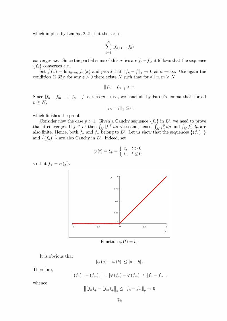
which implies by Lemma 2.21 that the series

∞Xk=1

(fk+1 − fk)

converges a.e.. Since the partial sums of this series are fn−f1, it follows that the sequencefn converges a.e..Set f (x) = limn→∞ fn (x) and prove that kfn − fk1 → 0 as n → ∞. Use again the

condition (2.32): for any ε > 0 there exists N such that for all n,m ≥ N

kfn − fmk1 < ε.

Since |fn − fm| → |fn − f | a.e. as m → ∞, we conclude by Fatou’s lemma that, for alln ≥ N ,

kfn − fk1 ≤ ε,

which finishes the proof.Consider now the case p > 1. Given a Cauchy sequence fn in Lp, we need to prove

that it converges. If f ∈ Lp thenRM|f |p dμ <∞ and, hence,

RMfp+ dμ and

RMfp− dμ are

also finite. Hence, both f+ and f− belong to Lp. Let us show that the sequences©(fn)+

ªand

©(fn)−

ªare also Cauchy in Lp. Indeed, set

ϕ (t) = t+ =

½t, t > 0,0, t ≤ 0,

so that f+ = ϕ (f).

52.50-2.5-5

5

3.75

2.5

1.25

0

x

y

x

y

Function ϕ (t) = t+

It is obvious that|ϕ (a)− ϕ (b)| ≤ |a− b| .

Therefore, ¯(fn)+ − (fm)+

¯= |ϕ (fn)− ϕ (fm)| ≤ |fn − fm| ,

whence °°(fn)+ − (fm)+°°p ≤ kfn − fmkp → 0

74

as n,m→∞. This proves that the sequence©(fn)+

ªis Cauchy, and the same argument

applies to©(fn)−

ª.

It suffices to prove that each sequence©(fn)+

ªand

©(fn)−

ªconverges in Lp. Indeed,

if we know already that (fn)+ → g and (fn)− → h in Lp then

fn = (fn)+ − (fn)− → g − h.

Therefore, renaming each of the sequence©(fn)+

ªand

©(fn)−

ªback to fn, we can

assume in the sequel that fn ≥ 0.The fact that fn ∈ Lp implies that fpn ∈ L1. Let us show that the sequence fpn is

Cauchy in L1. For that we use the following elementary inequalities.

Claim. For all a, b ≥ 0

|a− b|p ≤ |ap − bp| ≤ p |a− b|¡ap−1 + bp−1

¢. (2.33)

If a = b then (2.33) is trivial. Assume now that a > b (the case a < b is symmetric).Applying the mean value theorem to the function ϕ (t) = tp, we obtain that, for someξ ∈ (b, a),

ap − bp = ϕ0 (ξ) (a− b) = pξp−1 (a− b) .

Observing that ξp−1 ≤ ap−1, we obtain the right hand side inequality of (2.33).The left hand side inequality in (2.33) amounts to

(a− b)p + bp ≤ ap,

which will follow from the following inequality

xp + yp ≤ (x+ y)p , (2.34)

that holds for all x, y ≥ 0. Indeed, without loss of generality, we can assume that x ≥ yand x > 0. Then, using the Bernoulli inequality, we obtain

(x+ y)p = xp³1 +

y

x

´p≥ xp

³1 + p

y

x

´≥ xp

³1 +

³yx

´p´= xp + yp.

Coming back to a Cauchy sequence fn in Lp such that fn ≥ 0, let us show that fpnis Cauchy in L1. We have by (2.33)

|fpn − fpm| ≤ p |fn − fm|¡fp−1n + fp−1m

¢.

Recall the Hölder inequalityZM

|fg| dμ ≤µZ

M

|f |p dμ¶1/pµZ

M

|g|q dμ¶1/q

,

where q is the Hölder conjugate to p, that is, 1p+ 1

q= 1. Using this inequality, we obtainZ

M

|fpn − fpm| dμ ≤ p

µZM

|fn − fm|p dμ¶1/pµZ

M

¡fp−1n + fp−1m

¢qdμ

¶1/q. (2.35)

75

To estimate the last integral, use the inequality

(x+ y)q ≤ 2q (xq + yq) ,

which yields ¡fp−1n + fp−1m

¢q ≤ 2q ¡f (p−1)qn + f (p−1)qm

¢= 2q (fpn + fpm) , (2.36)

where we have used the identity (p− 1) q = p. Note that the numerical sequencenkfnkp

ois bounded. Indeed, by the Minkowski inequality,¯

kfnkp − kfmkp¯≤ kfn − fmkp → 0

as n,m → ∞. Hence, the sequencenkfnkp

o∞n=1

is a numerical Cauchy sequence and,

hence, is bounded. Integrating (2.36) we obtain thatZM

¡fp−1n + fp−1m

¢qdμ ≤ 2q

µZM

fpn dμ+

ZM

fpm dμ

¶≤ const,

where the constant const is independent of n,m. Hence, by (2.35)ZM

|fpn − fpm| dμ ≤ constµZ

M

|fn − fm|p dμ¶1/p

= const kfn − fmkp → 0 as n,m→∞,

whence it follows that the sequence fpn is Cauchy in L1. By the first part of the proof,we conclude that this sequence converges to a function g ∈ L1. By Exercise 52, we haveg ≥ 0. Set f = g1/p and show that fn → f in Lp. Indeed, by (2.33) we haveZ

M

|fn − f |p dμ ≤ZM

|fpn − fp| dμ =ZM

|fpn − g| dμ→ 0

which was to be proved.Finally, there is also the space L∞ (that is, Lp with p = ∞), which is defined in

Exercise 56 and which is also complete.

2.8 Product measures and Fubini’s theorem

2.8.1 Product measure

Let M1,M2 be two non-empty sets and S1, S2 be families of subsets of M1 and M2,respectively. Consider on the set M =M1 ×M2 the family of subsets

S = S1 × S2 := A×B : A ∈ S1, B ∈ S2 .Recall that, by Exercise 6, if S1 and S2 are semi-rings then S1 × S2 is also a semi-ring.Let μ1 and μ2 be two two functionals on S1 and S2, respectively. As before, define

their product μ = μ1 × μ2 as a functional on S by

μ (A×B) = μ1 (A)μ2 (B) for all A ∈ S1, B ∈ S2.

By Exercise 20, if μ1 and μ2 are finitely additive measures on semi-rings S1 and S2 thenμ is finitely additive on S. We are going to prove (independently of Exercise 20), that ifμ1 and μ2 are σ-additive then so is μ. A particular case of this result whenM1 =M2 = Rand μ1 = μ2 is the Lebesgue measure was proved in Lemma 1.11 using specific propertiesof R. Here we consider the general case.

76

Theorem 2.22 Assume that μ1 and μ2 are σ-finite measures on semi-rings S1 and S2 onthe sets M1 and M2 respectively. Then μ = μ1× μ2 is a σ-finite measure on S = S1× S2.

By Carathéodory’s extension theorem, μ can be then uniquely extended to the σ-algebra of measurable sets on M . The extended measure is also denoted by μ1 × μ2 andis called the product measure of μ1 and μ2. Observe that the product measure is σ-finite(and complete). Hence, one can define by induction the product μ1 × ...× μn of a finitesequence of σ-finite measures μ1, ..., μn. Note that this product satisfies the associativelaw (Exercise 57).Proof. Let C,Cn be sets from S such that C =

FnCn where n varies in a finite or

countable set. We need to prove that

μ (C) =Xn

μ (Cn) . (2.37)

Let C = A×B and Cn = An×Bn where A,An ∈ S1 and B,Bn ∈ S2. Clearly, A =S

nAn

and B =S

nBn.Consider function fn on M1 defined by

fn (x) =

½μ2 (Bn) , x ∈ An,0, x /∈ An

that is fn = μ2 (Bn) 1An .Claim. For any x ∈ A, X

n

fn (x) = μ2 (B) . (2.38)

We have Xn

fn (x) =X

n:x∈An

fn (x) =X

n:x∈An

μ2 (Bn) .

If x ∈ An and x ∈ Am and n 6= m then the sets Bn, Bm must be disjoint. Indeed, ify ∈ Bn ∩ Bm then (x, y) ∈ Cn ∩ Cm, which contradicts the hypothesis that Cn, Cm aredisjoint. Hence, all sets Bn with the condition x ∈ An are disjoint. Furthermore, theirunion is B because the set x ×B is covered by the union of the sets Cn. Hence,X

n:x∈An

μ2 (Bn) = μ2

µ Fn:x∈An

Bn

¶= μ2 (B) ,

which finishes the proof of the Claim.Integrating the identity (2.38) over A, we obtainZ

A

ÃXn

fn

!dμ1 = μ2 (B) μ1 (A) = μ (C) .

On the other hand, since fn ≥ 0, the partials sums of the seriesP

n fn form an increasingsequence. Applying the monotone convergence theorem to the partial sums, we obtainthat the integral is interchangeable with the infinite sum, whenceZ

A

ÃXn

fn

!dμ1 =

Xn

ZA

fn dμ1 =Xn

μ2 (Bn)μ1 (An) =Xn

μ (Cn) .

77

Comparing the above two lines, we obtain (2.37).Finally, let us show that measure μ is σ-finite. Indeed, since μ1 and μ2 are σ-finite,

there are sequences An ⊂ S1 and Bn ⊂ S2 such that μ1 (An) <∞, μ2 (Bn) <∞ andSnAn = M1,

SnBn = M2. Set Cnm = An ×Bm. Then μ (Cnm) = μ1 (An)μ2 (Bm) <∞

andS

n,mCnm =M . Since the sequence Cnm is countable, we conclude that measure μis σ-finite.

2.8.2 Cavalieri principle

Before we state the main result, let us discuss integration of functions taking value ∞.Let μ be an complete σ-finite measure on a set M and let f be a measurable function onM with values in [0,∞]. If the set

S := x ∈M : f (x) =∞

has measure 0 then there is no difficulty in definingRMf dμ since the function f can be

modified on set S to have finite values. If μ (S) > 0 then we define the integral of f byZM

f dμ =∞. (2.39)

For example, let f be a simple function, that is, f =P

k ak1Akwhere ak ∈ [0,∞] are

distinct values of f . Assume that one of ak is equal to∞. Then S = Ak with this k, andif μ (Ak) > 0 then X

k

akμ (Ak) =∞,

which matches the definition (2.39).Many properties of integration remain true if the function under the integral is allowed

to take value∞. We need the following extension of the monotone convergence theorem.Extended monotone convergence theorem If fk∞k=1 is an increasing sequence ofmeasurable functions on M taking values in [0,∞] and fk → f a.e. as k →∞ thenZ

M

f dμ = limk→∞

ZM

fk dμ. (2.40)

Proof. Indeed, if f is finite a.e. then this was proved in Theorem 2.15. Assume thatf = ∞ on a set of positive measure. If one of fk is also equal to ∞ on a set of positivemeasure then

RMfk dμ =∞ for large enough k and the both sides of (2.40) are equal to

∞. Consider the remaining case when all fk are finite a.e.. Set

C = limk→∞

ZM

fk dμ.

We need to prove that C =∞. Assume from the contrary that C <∞. Then, for all k,ZM

fk dμ ≤ C,

and by the second monotone convergence theorem (Theorem 2.16) we conclude thatthe limit f (x) = limk→∞ fk (x) is finite a.e., which contradicts the assumption thatμ f =∞ > 0.

78

Now, let μ1 and μ2 be σ-finite measures defined on σ-algebras M1 and M2 on setsM1,M2. Let μ = μ1 × μ2 be the product measure on M =M1 ×M2, which is defined ona σ-algebraM. Consider a set A ∈M and, for any x ∈ M consider the x-section of A,that is, the set

Ax = y ∈M2 : (x, y) ∈ A .Define the following function on M1:

ϕA (x) =

½μ2 (Ax) , if Ax ∈M2,0 otherwise

(2.41)

Theorem 2.23 (The Cavalieri principle) If A ∈M then, for almost all x ∈M1, the setAx is a measurable subset of M2 (that is, Ax ∈M2), the function ϕA (x) is measurableon M1, and

μ (A) =

ZM1

ϕA dμ1. (2.42)

Note that the function ϕA (x) takes values in [0,∞] so that the above discussion ofthe integration of such functions applies.

Example. The formula (2.42) can be used to evaluate the areas in R2 (and volumes inRn). For example, consider a measurable function function ϕ : (a, b) → [0,+∞) and letA be the subgraph of ϕ, that is,

A =©(x, y) ∈ R2 : a < x < b, 0 ≤ y ≤ ϕ (x)

ª.

Considering R2 as the product R×R, and the two-dimensional Lebesgue measure λ2 asthe product λ1 × λ1, we obtain

ϕA (x) = λ1 (Ax) = λ1 [0, ϕ (x)] = ϕ (x) ,

provided x ∈ (a, b) and ϕA (x) = 0 otherwise. Hence,

λ2 (A) =

Z(a,b)

ϕdλ1.

If ϕ is Riemann integrable then we obtain

λ2 (A) =

Z b

a

ϕ (x) dx,

which was also proved in Exercise 23.

Proof of Theorem 2.23. Denote by A the family of all sets A ∈M for which allthe claims of Theorem 2.23 are satisfied. We need to prove that A =M.Consider first the case when the measures μ1, μ2 are finite. The finiteness of measure μ2

implies, in particular, that the function ϕA (x) is finite. Let show thatA ⊃ S :=M1×M2

(note that S is a semi-ring). Indeed, any set A ∈ S has the form A = A1 × A2 whereAi ∈Mi. Then we have

Ax =

½A2, x ∈ A1,∅, x /∈ A1,

∈M2,

79

ϕA (x) =

½μ2 (A2) , x ∈ A1,0, x /∈ A1,

so that ϕA is a measurable function on M1, andZM1

ϕA dμ1 = μ2 (A2)μ1 (A1) = μ (A) .

All the required properties are satisfied and, hence, A ∈ A.Let us show that A is closed under monotone difference (that is, A− = A). Indeed, if

A,B ∈ A and A ⊃ B then(A−B)x = Ax −Bx,

so that (A−B)x ∈M2 for almost all x ∈M1,

ϕA−B (x) = μ2 (Ax)− μ2 (Bx) = ϕA (x)− ϕB (x)

so that the function ϕA−B is measurable, andZM1

ϕA−B dμ1 =

ZM1

ϕA dμ1 −ZM1

ϕB dμ1 = μ (A)− μ (B) = μ (A−B) .

In the same way, A is closed under taking finite disjoint unions.Let us show that A is closed under monotone limits. Assume first that An ⊂ A is

an increasing sequence and let A = limn→∞An =S

nAn. Then

Ax =Sn

(An)x

so that Ax ∈M2 for almost all x ∈M1,

ϕA (x) = μ2 (Ax) = limn→∞

μ2 ((An)x) = limn→∞

ϕAn(x) .

In particular, ϕA is measurable as the pointwise limit of measurable functions. Since thesequence

©ϕAn

ªis monotone increasing, we obtain by the monotone convergence theoremZ

M1

ϕA dμ1 = limn→∞

ZM1

ϕAndμ1 = lim

n→∞μ (An) = μ (A) . (2.43)

Hence, A ∈ A. Note that this argument does not require the finiteness of measures μ1and μ2 because if these measures are only σ-finite and, hence, the functions ϕAk

are notnecessarily finite, the monotone convergence theorem can be replaced by the extendedmonotone convergence theorem. This remark will be used below.Let now An ⊂ A be decreasing and let A = limn→∞An =

TnAn. Then all the above

argument remains true, the only difference comes in justification of (2.43). We cannot usethe monotone convergence theorem, but one can pass to the limit under the sign of theintegral by the dominated convergence theorem because all functions ϕAn are bounded bythe function ϕA1, and the latter is integrable because it is bounded by μ2 (M2) and themeasure μ1 (M1) is finite.Let Σ be the minimal σ-algebra containing S. From the above properties of A, it

follows that A ⊃ Σ. Indeed, let R be the minimal algebra containing S, that is, Rconsists of finite disjoint union of elements of S. Since A contains S and A is closed

80

under taking finite disjoint unions, we conclude that A contains R. By Theorem 1.14,Σ = Rlim, that is, Σ is the extension of R by monotone limits. Since A is closed undermonotone limits, we conclude that A ⊃ Σ.To proceed further, we need a refinement of Theorem 1.10. The latter says that if

A ∈M then there is B ∈ Σ such that μ (A M B) = 0. In fact, set B can be chosen tocontain A, as is claimed in the following stronger statement.

Claim (Exercise 54) For any set A ∈ M, there is a set B ∈ Σ such that B ⊃ A andμ (B −A) = 0.Using this Claim, let us show that A contains sets of measure 0. Indeed, for any set

A such that μ (A) = 0, there is B ∈ Σ such that A ⊂ B and μ (B) = 0 (the latter beingequivalent to μ (B −A) = 0). It follows thatZ

M1

ϕB dμ1 = μ (B) = 0,

which implies that μ2 (Bx) = ϕB (x) = 0 for almost all x ∈M1. Since Ax ⊂ Bx, it followsthat μ2 (Ax) = 0 for almost all x ∈M1. In particular, the set Ax is measurable for almostall x ∈M1. Furthermore, we have ϕA (x) = 0 a.e. and, hence,Z

M1

ϕA dμ1 = 0 = μ (A) ,

which implies that A ∈ A.Finally, let us show that A =M. By the above Claim, for any set A ∈M, there is

B ∈ Σ such that B ⊃ A and μ (B −A) = 0. Then B ∈ A by the previous argument, andthe set C = B − A is also in A as a set of measure 0. Since A = B − C and A is closedunder monotone difference, we conclude that A ∈ A.Consider now the general case of σ-finite measures μ1, μ2. Consider an increasing

sequences Mik∞k=1 of measurable sets in Mi (i = 1, 2) such that μi (Mik) < ∞ andSkMik =Mi. Then measure μi is finite in Mik so that the first part of the proof applies

to setsAk = A ∩ (M1k ×M2k) ,

so that Ak ∈ A. Note that Ak is an increasing sequence and A =S

k=1Ak. Since thefamily A is closed under increasing monotone limits, we obtain that A ∈ A, which finishesthe proof.

Example. Let us evaluate the area of the disc in R2

D =©(x, y) ∈ R2 : x2 + y2 < r2

ª,

where r > 0. We haveDx =

ny ∈ R : |y| <

√r2 − x2

oand

ϕD (x) = λ1 (Dx) = 2√r2 − x2,

81

provided |x| < r. If |x| ≥ r then Dx = ∅ and ϕD (x) = 0. Hence, by Theorem 2.23,

λ2 (D) =

Z r

−r2√r2 − x2dx

= 2r2Z 1

−1

√1− t2dt

= 2r2π

2= πr2.

Now let us evaluate the volume of the ball in R3

B =©(x, y, z) ∈ R3 : x2 + y2 + z2 < r2

ª.

We haveBx =

©(y, z) ∈ R2 : y2 + z2 < r2 − x2

ª,

which is a disk of radius√r2 − x2 in R2, whence

ϕB (x) = λ2 (Bx) = π¡r2 − x2

¢provided |x| < r, and ϕB (x) = 0 otherwise. Hence,

λ3 (B) =

Z r

−rπ¡r2 − x2

¢dx =

4

3πr3.

One can show by induction that if Bn (r) is the n-dimensional ball of radius r then

λn (Bn (r)) = cnrn

with some constant cn (see Exercise 59).

Example. Let B be a measurable subset of Rn−1 of a finite measure, p be a point in Rn

with pn > 0, and C be a cone over B with the pole at p defined by

C = (1− t) p+ ty : y ∈ B, 0 < t < 1 .

Let us show that

λn (C) =λn−1 (B) pn

n.

Considering Rn as the product R×Rn−1, we obtain, for any 0 < z < pn,

Cz = x ∈ C : xn = z = (1− t) p+ ty : y ∈ B, (1− t) pn = z= (1− t) p+ tB,

where t = 1− zpn; besides, if z /∈ (0, pn) then Cz = ∅. Hence, for any 0 < z < pn, we have

ϕz (C) = λn−1 (Cz) = tn−1λn−1 (B) ,

and

λn (C) = λn−1 (B)

Z pn

0

µ1− z

pn

¶n−1dz = λn−1 (B) pn

Z 1

0

sn−1ds =λn−1 (B) pn

n.

82

2.8.3 Fubini’s theorem

Theorem 2.24 (Fubini’s theorem) Let μ1 and μ2 be complete σ-finite measures on thesets M1, M2, respectively. Let μ = μ1 × μ2 be the product measure on M = M1 ×M2

and let f (x, y) be a measurable function on M with values in [0,∞], where x ∈ M1 andy ∈M2. Then Z

M

f dμ =

ZM1

µZM2

f (x, y) dμ2 (y)

¶dμ1 (x) . (2.44)

More precisely, the function y 7→ f (x, y) is measurable on M2 for almost all x ∈M1, thefunction

x 7→ZM2

f (x, y) dμ2

is measurable on M1, and its integral over M1 is equal toRMf dμ.

Furthermore, if f is a (signed) integrable function onM , then the function y 7→ f (x, y)is integrable on M2 for almost all x ∈M1, the function

x 7→ZM2

f (x, y) dμ2

is integrable on M1, and the identity (2.44) holds.

The first part of Theorem 2.24 dealing with non-negative functions is also called Ton-neli’s theorem. The expression on the right hand side of (2.44) is referred to as a repeated(or iterated) integral. Switching x and y in (2.44) yields the following identity, which istrue under the same conditions:Z

M

f dμ =

ZM2

µZM1

f (x, y) dμ1 (x)

¶dμ2 (y) .

By induction, this theorem extends to a finite product μ = μ1 × μ2 × ... × μn ofmeasures.Proof. Consider the product

fM =M × R =M1 ×M2 ×R

and measure eμ on fM , which is defined byeμ = μ× λ = μ1 × μ2 × λ,

where λ = λ1 is the Lebesgue measure on R (note that the product of measure satisfiesthe associative law — see Exercise 57). Consider the set A ⊂ fM , which is the subgraph offunction f , that is,

A =n(x, y, z) ∈ fM : 0 ≤ z ≤ f (x, y)

o(here x ∈M1, y ∈M2, z ∈ R). By Theorem 2.23, we have

μ (A) =

ZM

λ¡A(x,y)

¢dμ.

83

Since A(x,y) = [0, f (x, y)] and λ¡A(x,y)

¢= f (x, y), it follows that

μ (A) =

ZM

f dμ. (2.45)

On the other hand, we have fM =M1 × (M2 ×R)and eμ = μ1 × (μ2 × λ) .

Theorem 2.23 now says that

μ (A) =

ZM1

(μ2 × λ) (Ax) dμ1 (x)

whereAx = (y, z) : 0 ≤ f (x, y) ≤ z .

Applying Theorem 2.23 to the measure μ2 × λ, we obtain

(μ2 × λ) (Ax) =

ZM2

λ³(Ax)y

´dμ2 =

ZM2

f (x, y) dμ2 (y) .

Hence,

μ (A) =

ZM1

µZM2

f (x, y) dμ2 (y)

¶dμ1 (x) .

Comparing with (2.45), we obtain (2.44). The claims about the measurability of theintermediate functions follow from Theorem 2.23.Now consider the case when f is integrable. By definition, function f is integrable if

f+ and f− are integrable. By the first part, we haveZM

f+dμ =

ZM1

µZM2

f+ (x, y) dμ2 (y)

¶dμ1.

Since the left hand side here is finite, it follows that the function

F (x) =

ZM2

f+ (x, y) dμ2 (y)

is integrable and, hence, is finite a.e.. Consequently, the function f+ (x, y) is integrable iny for almost all x. In the same way, we obtainZ

M

f−dμ =

ZM1

µZM2

f− (x, y) dμ2 (y)

¶dμ1,

so that the function

G (x) =

ZM2

f− (x, y) dμ2 (y)

is integrable and, hence, is finite a.e.. Therefore, the function f− (x, y) is integrable in yfor almost all x. We conclude that f = f+ − f− is integrable in y for almost all x, thefunction Z

M2

f (x, y) dμ2 (y) = F (x)−G (x)

84

is integrable on M1, andZM1

µZM2

f (x, y) dμ2 (y)

¶dμ1 (x) =

ZM1

F dμ1 −ZM1

Gdμ1 =

ZM

f dμ.

Example. Let Q be the unit square in R2, that is,

Q =©(x, y) ∈ R2 : 0 < x < 1, 0 < y < 1

ª.

Let us evaluate ZQ

(x+ y)2 dλ2.

Since Q = (0, 1)× (0, 1) and λ2 = λ1 × λ1, we obtain by (2.44)ZQ

(x+ y)2 dλ2 =

Z 1

0

µZ 1

0

(x+ y)2 dx

¶dy

=

Z 1

0

"(x+ y)3

3

#10

dy

=

Z 1

0

(1 + y)3 − y3

3dy

=

Z 1

0

µy2 + y +

1

3

¶dy

=1

3+1

2+1

3=7

6.

85

3 Integration in Euclidean spaces and in probabilityspaces

3.1 Change of variables in Lebesgue integral

Recall the following rule of change of variable in a Riemann integral:Z b

a

f (x) dx =

Z β

α

f (ϕ (y))ϕ0 (y) dy

if ϕ is a continuously differentiable function on [α, β] and a = ϕ (α), b = ϕ (β).Let us rewrite this formula for Lebesgue integration. Assume that a < b and α < β.

If ϕ is an increasing diffeomorphism from [α, β] onto [a, b] then ϕ (α) = a, ϕ (β) = b, andwe can rewrite this formula for the Lebesgue integration:Z

[a,b]

f (x) dλ1 (x) =

Z[α,β]

f (ϕ (y)) |ϕ0 (y)| dλ1 (y) , (3.1)

where we have used that ϕ0 ≥ 0.If ϕ is a decreasing diffeomorphism from [α, β] onto [a, b] then ϕ (α) = b, ϕ (β) = a,

and we have insteadZ[a,b]

f (x) dλ1 (x) = −Z[α,β]

f (ϕ (y))ϕ0 (y) dλ1 (y)

=

Z[α,β]

f (ϕ (y)) |ϕ0 (y)| dλ1 (y)

where we have used that ϕ0 ≤ 0.Hence, the formula (3.1) holds in the both cases when ϕ is an increasing or decreasing

diffeomorphism. The next theorem generalizes (3.1) for higher dimensions.

Theorem 3.1 (Transformationsatz) Let μ = λn be the Lebesgue measure in Rn. Let U, Vbe open subsets of Rn and Φ : U → V be a diffeomorphism. Then, for any non-negativemeasurable function f : V → R, the function f Φ : U → R is measurable andZ

V

f dμ =

ZU

(f Φ) |detΦ0| dμ. (3.2)

The same holds for any integrable function f : V → R.

Recall that Φ : U → V is a diffeomorphism if the inverse mapping Φ−1 : V → Uexists and both Φ and Φ0 are continuously differentiable. Recall also that Φ0 is the totalderivative of Φ, which in this setting coincides with the Jacobi matrix, that is,

Φ0 = JΦ =

µ∂Φi

∂xj

¶n

i,j=1

.

Let us rewrite (3.2) in the form matching (3.1):ZV

f (x) dμ (x) =

ZU

f (Φ (y)) |detΦ0 (y)| dμ (y) . (3.3)

86

The formula (3.3) can be explained and memorized as follows. In order to evaluateRVf (x) dμ (x), one finds a suitable substitution x = Φ (y), which maps one-to-one y ∈ U

to x ∈ V , and substitutes x via Φ (y), using the rule

dμ (x) = |detΦ0 (y)| dμ (y) .

Using the notation dxdyinstead of Φ0 (y), this rule can also be written in the form

dμ (x)

dμ (y)=

¯det

dx

dy

¯, (3.4)

which is easy to remember. Although presently the identity (3.4) has no rigorous meaning,it can be turned into a theorem using a proper definition of the quotient dμ (x) /dμ (y).

Example. Let Φ : Rn → Rn be a linear mapping that is, Φ (y) = Ay where A is anon-singular n× n matrix. Then Φ0 (y) = A and (3.2) becomesZ

Rnf (x) dμ = |detA|

ZRn

f (Ay) dμ (y) .

In particular, applying this to f = 1S where S is a measurable subset of Rn, we obtain

μ (S) = |detA|μ¡A−1S

¢or, renaming A−1S to S,

μ (AS) = |detA|μ (S) . (3.5)

In particular, if |detA| = 1 then μ (AS) = μ (S) that is, the Lebesgue measure is preservedby such linear mappings. Since all orthogonal matrices have determinants ±1, it followsthat the Lebesgue measure is preserved by orthogonal transformations of Rn, in particular,by rotations.

Example. Let S be the unit cube, that is,

S = x1e1 + ...+ xnen : 0 < xi < 1, i = 1, ..., n ,

where e1, ..., en the canonical basis in Rn. Setting ai = Aei, we obtain

AS = x1a1 + ...+ xnan : 0 < xi < 1, i = 1, ..., n .

This set is called a parallelepiped spanned by the vectors a1, ..., an (its particular case forn = 2 is a parallelogram). Denote it by Π (a1, ..., an). Note that the columns of the matrixA are exactly the column-vectors ai. Therefore, we obtain that from (3.5)

μ (Π (a1, ..., an)) = |detA| = |det (a1, a2, ..., an)| .

Example. Consider a tetrahedron spanned by a1, ..., an, that is,

T (a1, ..., an) = x1a1 + ...+ xnan : x1 + x2 + ...+ xn < 1, xi > 0, i = 1, ..., n .

87

It is possible to prove that

μ (T (a1, ..., an)) =1

n!|det (a1, a2, ..., an)|

(see Exercise 58).

Example. (The polar coordinates) Let (r, θ) be the polar coordinates in R2. The changefrom the Cartesian coordinates (x, y) to the polar coordinates (r, θ) can be regarded as amapping

Φ : U → R2

where U = (r, θ) : r > 0, − π < θ < π and

Φ (r, θ) = (r cos θ, r sin θ) .

The image of U is the open set

V = R2 \ (x, 0) : x ≤ 0 ,

and Φ is a diffeomorphism between U and V . We have

Φ0 =

µ∂rΦ1 ∂θΦ1∂rΦ2 ∂θΦ2

¶=

µcos θ −r sin θsin θ r cos θ

¶whence

detΦ0 = r.

Hence, we obtain the formula for computing the integrals in the polar coordinates:ZV

f (x, y) dλ2 (x, y) =

ZU

f (r cos θ, r sin θ) rλ2 (r, θ) . (3.6)

If function f is given on R2 then ZR2fdλ2 =

ZV

fdλ2

because the difference R2 \ V has measure 0. Also, using Fubini’s theorem in U , we canexpress the right hand side of (3.6) via repeated integrals and, hence, obtainZ

R2f (x, y) dλ2 (x, y) =

Z ∞

0

µZ π

−πf (r cos θ, r sin θ) dθ

¶rdr. (3.7)

For example, if f = 1D where D = (x, y) : x2 + y2 < R2 is the disk of radius R then

λ2 (D) =

ZR21D (x, y) dλ2 =

Z R

0

µZ π

−πdθ

¶rdr = 2π

Z R

0

rdr = πR2.

Example. Let us evaluate the integral

I =

Z ∞

−∞e−x

2

dx.

88

Using Fubini’s theorem, we obtain

I2 =

µZ ∞

−∞e−x

2

dx

¶µZ ∞

−∞e−y

2

dy

¶=

Z ∞

−∞

µZ ∞

−∞e−y

2

dy

¶e−x

2

dx

=

Z ∞

−∞

µZ ∞

−∞e−(x

2+y2)dy

¶dx

=

ZR2e−(x

2+y2)dλ2 (x, y) .

Then by (3.7)ZR2e−(x

2+y2)dλ2 =

Z ∞

0

µZ π

−πe−r

2

dθ

¶rdr = 2π

Z ∞

0

e−r2

rdr = π

Z ∞

0

e−r2

dr2 = π.

Hence, I2 = π and I =√π, that is,Z ∞

−∞e−x

2

dx =√π.

The proof of Theorem 3.1 will be preceded by a number of auxiliary claims.We say that a mapping Φ is good if (3.2) holds for all non-negative measurable func-

tions. Theorem 3.1 will be proved if we show that all diffeomorphisms are good.Claim 0. Φ is good if and only if for any measurable set B ⊂ V , the set A = Φ−1 (B) isalso measurable and

μ (B) =

ZA

|detΦ0| dμ. (3.8)

Proof. Applying (3.2) for indicator functions, that is, for functions f = 1B where Bis a measurable subset of V , we obtain that the function 1A = 1B Φ is measurable and

μ (B) =

ZU

1B (Φ (y)) |detΦ0 (y)| dμ (y) =ZU

1A (y) |detΦ0| dμ =ZA

|detΦ0| dμ. (3.9)

Conversely, if (3.8) is true then (3.2) is true for indicators functions f = 1B. By thelinearity of the integral and the monotone convergence theorem for series, we obtain (3.2)for simple functions:

f =∞Xk=1

bk1Bk.

Finally, any non-negative measurable function f is an increasing pointwise limit of simplefunctions, whence (3.2) follows for f .The idea of the proof of (3.8). We will first prove it for affine mappings, that is,

the mappings of the formΨ (x) = Cx+D

where C is a constant n × n matrix and D ∈ Rn. A general diffeomorphism Φ can beapproximated in a neighborhood of any point x0 ∈ U by the tangent mapping

Ψx0 (x) = Φ (x0) + Φ0 (x0) (x− x0) ,

89

which is affine. This implies that if A is a set in a small neighborhood of x0 then

μ (Φ (A)) ≈ μ (Ψx0 (A)) =

ZA

¯detΨ0

x0

¯dμ ≈

ZA

|detΦ0| dμ.

Now split an arbitrary measurable set A ⊂ U into small pieces Ak∞k=1 and apply theprevious approximate identity to each Ak:

μ (Φ (A)) =Xk

μ (Φ (Ak)) ≈Xk

ZAk

|detΦ0| dμ =ZA

|detΦ0| dμ.

The error of approximation can be made arbitrarily small using finer partitions of A.

Claim 1. If Φ : U → V and Ψ : V →W are good mappings then Ψ Φ is also good.Proof. Let f : W → R be a non-negative measurable function. We need to prove

that ZW

f dμ =

ZU

(f Ψ Φ)¯det (Ψ Φ)0

¯dμ.

Since Ψ is good, we have ZW

f dμ =

ZV

(f Ψ) |detΨ0| dμ.

Set g = f Ψ |detΦ0| so that g is a function on V . Since Φ is good, we haveZV

g dμ =

ZU

(g Φ) |detΦ0| dμ.

Combining these two lines and using the chain rule in the form

(Ψ Φ)0 = (Ψ0 Φ)Φ0

and it its consequencedet (Ψ Φ)0 = det (Ψ0 Φ) detΦ0,

we obtain ZW

f dμ =

ZU

(f Ψ Φ) |detΨ0 Φ| |detΦ0| dμ

=

ZU

(f Ψ Φ)¯det (Ψ Φ)0

¯dμ,

which was to be proved

Claim 2. All translations Rn are good.Proof. A translation of Rn is a mapping of the form Φ (x) = x + v where v is a

constant vector from Rn. Obviously, Φ0 = id and detΦ0 ≡ 1. Hence, the fact that Φ isgood amounts by (3.8) to

μ (B) = μ (B − ν) ,

for any measurable subset B ⊂ Rn. This is obviously true when B is a box. Thenfollowing the procedure of construction of the Lebesgue measure, we obtain that this istrue for any measurable set B.

90

Note that the identity (3.2) for translations amounts toZRn

f (x) dμ (x) =

ZRn

f (y + v) dμ (y) , (3.10)

for any non-negative measurable function f on Rn.

Claim 3. All homotheties of Rn are good.Proof. A homothety of Rn is a mapping Φ (x) = cx where c is a non-zero real. Since

Φ0 = c id and, hence, detΦ0 = cn, the fact that Φ is good is equivalent to the identity

μ (B) = |c|n μ¡c−1B

¢, (3.11)

for any measurable set B ⊂ Rn. This is true for boxes and then extends to all measurablesets by the measure extension procedure.The identity (3.2) for homotheties amounts toZ

Rnf (x) dμ (x) = |c|n

ZRn

f (cy) dμ (y) , (3.12)

for any non-negative measurable function f on Rn.

Claim 4. All linear mappings are good.Proof. Let Φ be a linear mapping from Rn to Rn. Extending a function f , initially

defined on V , to the whole Rn by setting f = 0 in Rn\V , we can assume that V = U = Rn.Let us use the fact from linear algebra that any non-singular linear mapping can be reducedby column-reduction of the matrices to the composition of finitely many elementary linearmappings, where an elementary linear mapping is one of the following:

1. Φ (x1, . . . , xn) = (cx1, x2, . . . , xn) for some c 6= 0;

2. Φ (x1, . . . , xn) = (x1 + cx2, x2, . . . , xn) ;

3. Φ (x1, . . . , xi, . . . , xj, . . . , xn) = (x1, . . . , xj, . . . , xi, . . . , xn) (switching the variablesxi and xj).

Hence, in the view of Claim 1, it suffices to prove Claim 4 if Φ is an elementarymapping. If Φ is of the first type then, using Fubini’s theorem and setting λ = λ1, we canwrite Z

Rnf dμ =

ZR. . .

ZR

µZRf (x1, ..., xn) dλ (x1)

¶dλ (x2) . . . dλ (xn)

=

ZR. . .

ZR

µZRf (ct, ..., xn) |c| dλ (t)

¶dλ (x2) . . . dλ (xn)

=

ZRn

f (cx1, x2, . . . , xn) |c| dμ

=

ZRn

f (Φ (x)) |detΦ0| dμ,

where we have used the change of integral under a homothety in R1 and detΦ0 = c.

91

If Φ is of the second type thenZRn

f dμ =

ZR. . .

ZR

µZRf (x1, ..., xn) dλ (x1)

¶dλ (x2) . . . dλ (xn)

=

ZR. . .

ZR

µZRf (x1 + cx2, ..., xn) dλ (x1)

¶dλ (x2) . . . dλ (xn)

=

ZRn

f (x1 + cx2, x2, . . . , xn) dμ

=

ZRn

f (Φ (x)) |detΦ0| dμ,

where we have used the translation invariance of the integral in R1 and detΦ0 = 1.Let Φ be of the third type. For simplicity of notation, let

Φ (x1, x2, . . . , xn) = (x2, x1, . . . , xn) .

Then, using twice Fubini’s theorem with different orders of the repeated integrals, weobtain Z

Rnf dμ =

ZR. . .

ZR

µZRf (x1, x2, ..., xn) dλ (x2)

¶dλ (x1) . . . dλ (xn)

=

ZR. . .

ZR

µZRf (y2, y1, y3.., yn) dλ (y1)

¶dλ (y2) . . . dλ (yn)

=

ZRn

f (y2, y1, . . . , yn) dμ (y)

=

ZRn

f (Φ (y)) |detΦ0| dμ.

In the second line we have changed notation y1 = x2, y2 = x1, yk = xk for k > 2 (let usemphasize that this is not a change of variable but just a change of notation in each ofthe repeated integrals), and in the last line we have used detΦ0 = −1.It follows from Claims 1, 2 and 4 that all affine mappings are good.It what follows we will use the ∞-norm in Rn:

kxk = kxk∞ := max1≤i≤n

|xi| .

Let Φ be a diffeomorphism between open sets U and V in Rn. Let K be a compact subsetof U .

Claim 5. For any η > 0 there is δ > 0 such that, for any interval [x, y] ⊂ K with thecondition ky − xk < δ, the following is true:

kΦ (y)− Φ (x)−Φ0 (x) (y − x) k ≤ ηky − xk.

Proof. Consider the function

f (t) = Φ ((1− t)x+ ty) , 0 ≤ t ≤ 1,

92

so that f (0) = Φ (x) and f (1) = Φ (y). Since the interval [x, y] is contained in U , thefunction f is defined for all t ∈ [0, 1]. By the fundamental theorem of calculus, we have

Φ (y)− Φ (x) =

Z 1

0

f 0 (t) dt =

Z 1

0

Φ0 ((1− t)x+ ty) (y − x) dt.

Since the function Φ0 (x) is uniformly continuous on K, δ can be chosen so that

x, z ∈ K, kz − xk < δ ⇒ kΦ (z)− Φ (x) k < η.

Applying this with z = (1− t)x+ ty and noticing that kz− xk ≤ ky− xk < δ, we obtain

kΦ0 ((1− t)x+ ty)− Φ0 (x) k < η.

DenotingF (t) = Φ0 ((1− t)x+ ty)−Φ0 (x) ,

we obtain

Φ (y)−Φ (x) =

Z 1

0

(Φ0 (x) + F (t)) (y − x) dt

= Φ0 (x) (y − x) +

Z 1

0

F (t) (y − x) dt

and

kΦ (y)− Φ (x)−Φ0 (x) (y − x) k = kZ 1

0

F (t) (y − x) kdt ≤ ηky − xk.

For any x ∈ U , denote by Ψx (y) the tangent mapping of Φ at x, that is,

Ψx (y) = Φ (x) + Φ0 (x) (y − x) . (3.13)

Clearly, Ψx is a non-singular affine mapping in Rn. In particular, Ψx is good. Note alsothat Ψx (x) = Φ (x) and Ψ0x ≡ Φ0 (x) .The Claim 5 can be stated as follows: for any η > 0 there is δ > 0 such that if

[x, y] ⊂ K and ky − xk < δ then

kΦ (y)−Ψx (y)k ≤ η ky − xk . (3.14)

Consider a metric balls Qr (x) with respect to the ∞-norm, that is,

Qr (x) = y ∈ Rn : ky − xk < r .

Clearly, Qr (x) is the cube with the center x and with the edge length 2r. If Q = Qr (x)and c > 0 then set cQ = Qcr (x).

Claim 6. For any ε ∈ (0, 1), there is δ > 0 such that, for any cube Q = Qr (x) ⊂ K withradius 0 < r < δ,

Ψx ((1− ε)Q) ⊂ Φ (Q) ⊂ Ψx ((1 + ε)Q) . (3.15)

93

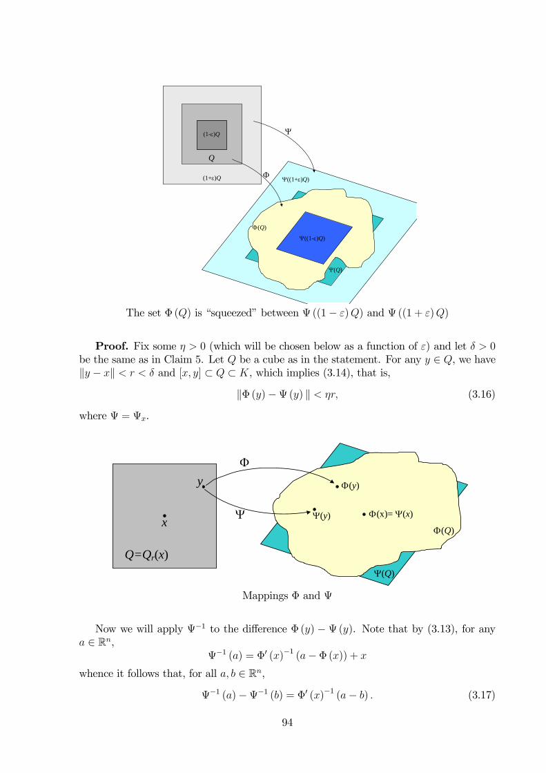
Ψ

Φ

Φ(Q)

Ψ((1-ε)Q)

Ψ((1+ε)Q)

Ψ(Q)

Q

(1-ε)Q

(1+ε)Q

The set Φ (Q) is “squeezed” between Ψ ((1− ε)Q) and Ψ ((1 + ε)Q)

Proof. Fix some η > 0 (which will be chosen below as a function of ε) and let δ > 0be the same as in Claim 5. Let Q be a cube as in the statement. For any y ∈ Q, we haveky − xk < r < δ and [x, y] ⊂ Q ⊂ K, which implies (3.14), that is,

kΦ (y)−Ψ (y) k < ηr, (3.16)

where Ψ = Ψx.

Φ

Ψ

Q=Qr(x)

Ψ(y)

Φ(y)

Φ(x)= Ψ(x) x

y

Ψ(Q)

Φ(Q)

Mappings Φ and Ψ

Now we will apply Ψ−1 to the difference Φ (y) − Ψ (y). Note that by (3.13), for anya ∈ Rn,

Ψ−1 (a) = Φ0 (x)−1 (a−Φ (x)) + x

whence it follows that, for all a, b ∈ Rn,

Ψ−1 (a)−Ψ−1 (b) = Φ0 (x)−1 (a− b) . (3.17)

94

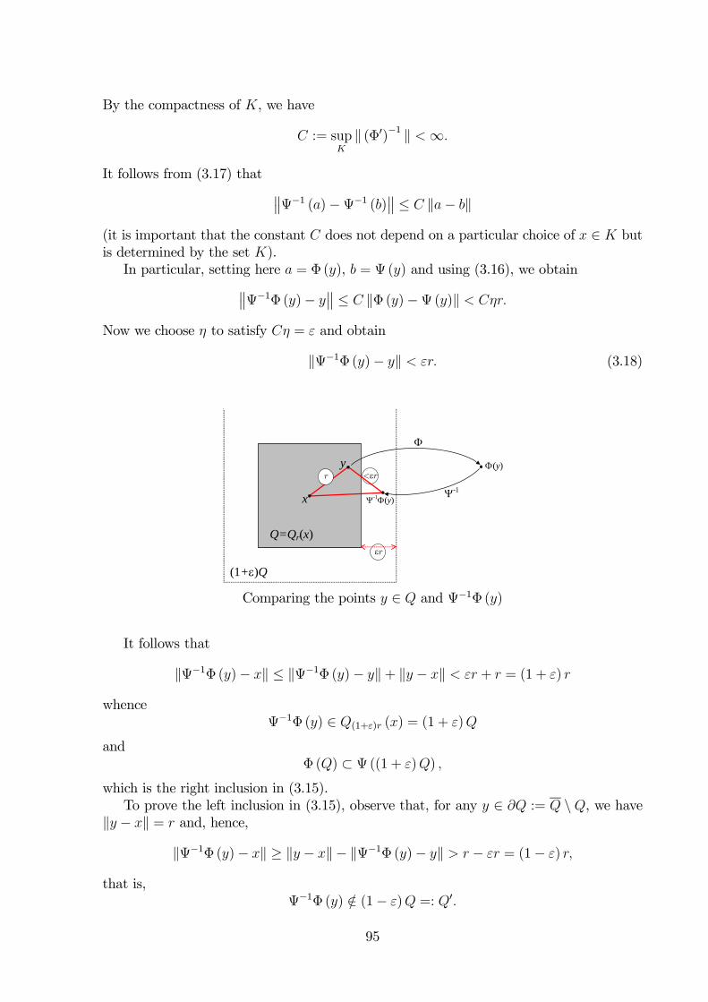
By the compactness of K, we have

C := supKk (Φ0)−1 k <∞.

It follows from (3.17) that °°Ψ−1 (a)−Ψ−1 (b)°° ≤ C ka− bk

(it is important that the constant C does not depend on a particular choice of x ∈ K butis determined by the set K).In particular, setting here a = Φ (y), b = Ψ (y) and using (3.16), we obtain°°Ψ−1Φ (y)− y

°° ≤ C kΦ (y)−Ψ (y)k < Cηr.

Now we choose η to satisfy Cη = ε and obtain

kΨ−1Φ (y)− yk < εr. (3.18)

Φ

Ψ-1

Q=Qr(x)

Φ(y)

x

y

Ψ-1Φ(y)

r <εr

(1+ε)Q

εr

Comparing the points y ∈ Q and Ψ−1Φ (y)

It follows that

kΨ−1Φ (y)− xk ≤ kΨ−1Φ (y)− yk+ ky − xk < εr + r = (1 + ε) r

whenceΨ−1Φ (y) ∈ Q(1+ε)r (x) = (1 + ε)Q

andΦ (Q) ⊂ Ψ ((1 + ε)Q) ,

which is the right inclusion in (3.15).To prove the left inclusion in (3.15), observe that, for any y ∈ ∂Q := Q \Q, we have

ky − xk = r and, hence,

kΨ−1Φ (y)− xk ≥ ky − xk− kΨ−1Φ (y)− yk > r − εr = (1− ε) r,

that is,Ψ−1Φ (y) /∈ (1− ε)Q =: Q0.

95

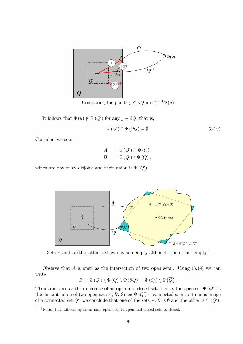
Φ

Ψ-1

Q

Φ(y)

x

y

Ψ-1Φ(y)

r<εr

Q εr

Comparing the points y ∈ ∂Q and Ψ−1Φ (y)

It follows that Φ (y) /∈ Ψ (Q0) for any y ∈ ∂Q, that is,

Ψ (Q0) ∩ Φ (∂Q) = ∅. (3.19)

Consider two sets

A = Ψ (Q0) ∩ Φ (Q) ,B = Ψ (Q0) \ Φ (Q) ,

which are obviously disjoint and their union is Ψ (Q0).

Φ

Ψ

Q

Φ(x)= Ψ(x) x

Ψ(Q)

Φ(Q)

Q

Β = Ψ(Q)∖Φ(Q)

Α = Ψ(Q)∩Φ(Q)

Sets A and B (the latter is shown as non-empty although it is in fact empty)

Observe that A is open as the intersection of two open sets1. Using (3.19) we canwrite

B = Ψ (Q0) \ Φ (Q) \ Φ (∂Q) = Ψ (Q0) \ Φ¡Q¢.

Then B is open as the difference of an open and closed set. Hence, the open set Ψ (Q0) isthe disjoint union of two open sets A,B. Since Ψ (Q0) is connected as a continuous imageof a connected set Q0, we conclude that one of the sets A,B is ∅ and the other is Ψ (Q0).

1Recall that diffeomorphisms map open sets to open and closed sets to closed.

96

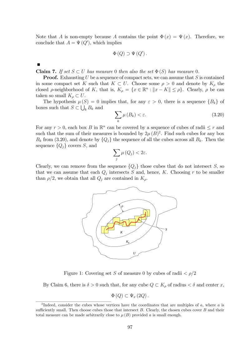
Note that A is non-empty because A contains the point Φ (x) = Ψ (x). Therefore, weconclude that A = Ψ (Q0), which implies

Φ (Q) ⊃ Ψ (Q0) .

Claim 7. If set S ⊂ U has measure 0 then also the set Φ (S) has measure 0.Proof. Exhausting U be a sequence of compact sets, we can assume that S is contained

in some compact set K such that K ⊂ U . Choose some ρ > 0 and denote by Kρ theclosed ρ-neighborhood of K, that is, Kρ = x ∈ Rn : kx−Kk ≤ ρ. Clearly, ρ be cantaken so small Kρ ⊂ U .The hypothesis μ (S) = 0 implies that, for any ε > 0, there is a sequence Bk of

boxes such that S ⊂S

kBk and Xk

μ (Bk) < ε. (3.20)

For any r > 0, each box B in Rn can be covered by a sequence of cubes of radii ≤ r andsuch that the sum of their measures is bounded by 2μ (B)2. Find such cubes for any boxBk from (3.20), and denote by Qj the sequence of all the cubes across all Bk. Then thesequence Qj covers S, and X

j

μ (Qj) < 2ε.

Clearly, we can remove from the sequence Qj those cubes that do not intersect S, sothat we can assume that each Qj intersects S and, hence, K. Choosing r to be smallerthan ρ/2, we obtain that all Qj are contained in Kρ.

K

Kρ

U

ρ

S

Figure 1: Covering set S of measure 0 by cubes of radii < ρ/2

By Claim 6, there is δ > 0 such that, for any cube Q ⊂ Kρ of radius < δ and center x,

Φ (Q) ⊂ Ψx (2Q) .

2Indeed, consider the cubes whose vertices have the coordinates that are multiples of a, where a issufficiently small. Then choose cubes those that intersect B. Clearly, the chosen cubes cover B and theirtotal measure can be made arbitrarily close to μ (B) provided a is small enough.

97

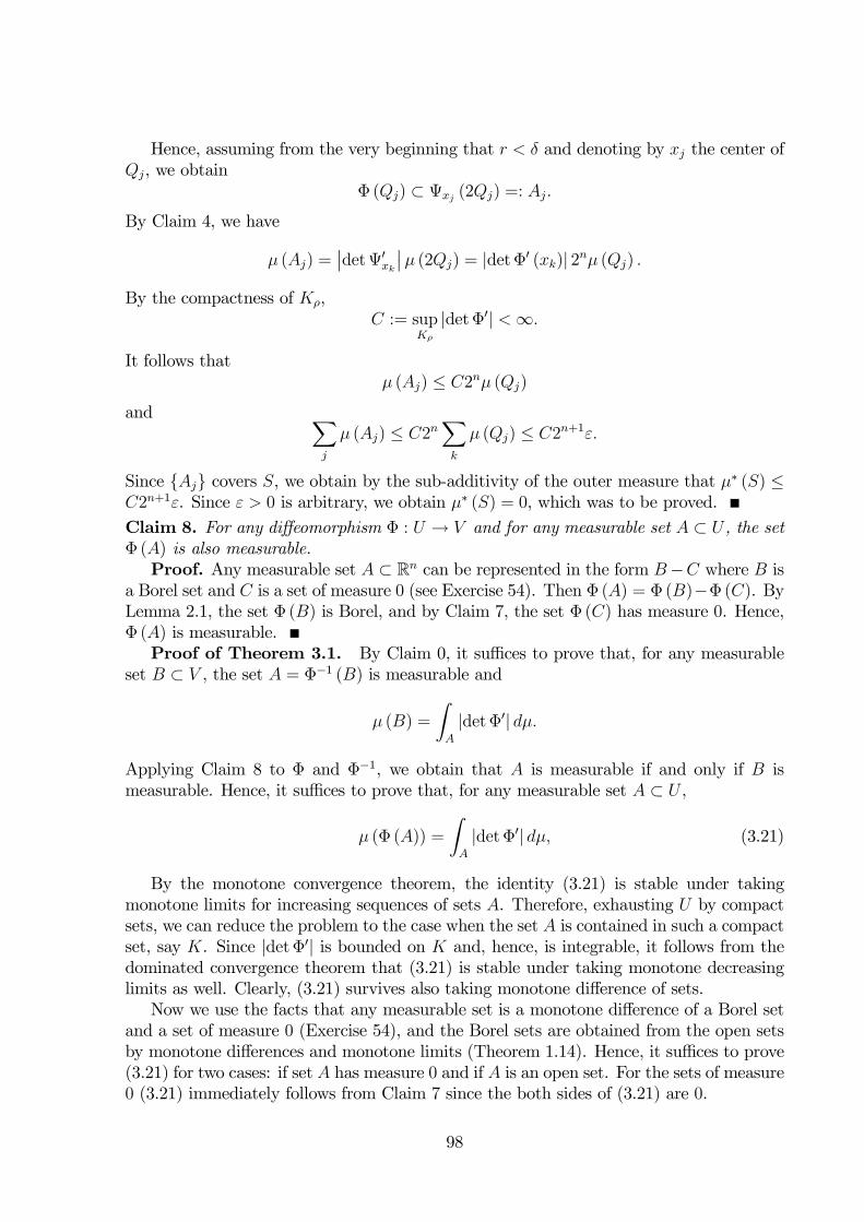
Hence, assuming from the very beginning that r < δ and denoting by xj the center ofQj, we obtain

Φ (Qj) ⊂ Ψxj (2Qj) =: Aj.

By Claim 4, we have

μ (Aj) =¯detΨ0xk

¯μ (2Qj) = |detΦ0 (xk)| 2nμ (Qj) .

By the compactness of Kρ,C := sup

Kρ

|detΦ0| <∞.

It follows thatμ (Aj) ≤ C2nμ (Qj)

and Xj

μ (Aj) ≤ C2nXk

μ (Qj) ≤ C2n+1ε.

Since Aj covers S, we obtain by the sub-additivity of the outer measure that μ∗ (S) ≤C2n+1ε. Since ε > 0 is arbitrary, we obtain μ∗ (S) = 0, which was to be proved.

Claim 8. For any diffeomorphism Φ : U → V and for any measurable set A ⊂ U , the setΦ (A) is also measurable.Proof. Any measurable set A ⊂ Rn can be represented in the form B−C where B is

a Borel set and C is a set of measure 0 (see Exercise 54). Then Φ (A) = Φ (B)−Φ (C). ByLemma 2.1, the set Φ (B) is Borel, and by Claim 7, the set Φ (C) has measure 0. Hence,Φ (A) is measurable.Proof of Theorem 3.1. By Claim 0, it suffices to prove that, for any measurable

set B ⊂ V , the set A = Φ−1 (B) is measurable and

μ (B) =

ZA

|detΦ0| dμ.

Applying Claim 8 to Φ and Φ−1, we obtain that A is measurable if and only if B ismeasurable. Hence, it suffices to prove that, for any measurable set A ⊂ U ,

μ (Φ (A)) =

ZA

|detΦ0| dμ, (3.21)

By the monotone convergence theorem, the identity (3.21) is stable under takingmonotone limits for increasing sequences of sets A. Therefore, exhausting U by compactsets, we can reduce the problem to the case when the set A is contained in such a compactset, say K. Since |detΦ0| is bounded on K and, hence, is integrable, it follows from thedominated convergence theorem that (3.21) is stable under taking monotone decreasinglimits as well. Clearly, (3.21) survives also taking monotone difference of sets.Now we use the facts that any measurable set is a monotone difference of a Borel set

and a set of measure 0 (Exercise 54), and the Borel sets are obtained from the open setsby monotone differences and monotone limits (Theorem 1.14). Hence, it suffices to prove(3.21) for two cases: if set A has measure 0 and if A is an open set. For the sets of measure0 (3.21) immediately follows from Claim 7 since the both sides of (3.21) are 0.

98

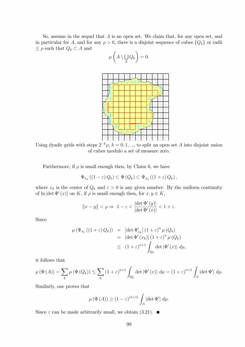
So, assume in the sequel that A is an open set. We claim that, for any open set, andin particular for A, and for any ρ > 0, there is a disjoint sequence of cubes Qk or radii≤ ρ such that Qk ⊂ A and

μ

µA \

Sk

Qk

¶= 0.

Using dyadic grids with steps 2−kρ, k = 0, 1, ..., to split an open set A into disjoint unionof cubes modulo a set of measure zero.

Furthermore, if ρ is small enough then, by Claim 6, we have

Ψxk ((1− ε)Qk) ⊂ Φ (Qk) ⊂ Ψxk ((1 + ε)Qk) ,

where xk is the center of Qk and ε > 0 is any given number. By the uniform continuityof ln |detΦ0 (x)| on K, if ρ is small enough then, for x, y ∈ K,

kx− yk < ρ⇒ 1− ε <|detΦ0 (y)||detΦ0 (x)| < 1 + ε.

Since

μ (Ψxk ((1 + ε)Qk)) =¯detΨ0xk

¯(1 + ε)n μ (Qk)

= |detΦ0 (xk)| (1 + ε)n μ (Qk)

≤ (1 + ε)n+1ZQk

det |Φ0 (x)| dμ,

it follows that

μ (Φ (A)) =Xk

μ (Φ (Qk)) ≤Xk

(1 + ε)n+1ZQk

det |Φ0 (x)| dμ = (1 + ε)n+1ZA

|detΦ0| dμ.

Similarly, one proves that

μ (Φ (A)) ≥ (1− ε)(n+1)ZA

|detΦ0| dμ.

Since ε can be made arbitrarily small, we obtain (3.21).

99

3.2 Random variables and their distributions

Recall that a probability space (Ω,F ,P) is a triple of a setΩ, a σ-algebraF (also frequentlycalled a σ-field) and a probability measure P on F , that is, a measure with the total mass1 (that is, P (Ω) = 1). Recall also that a function X : Ω → R is called measurable withrespect to F if for any x ∈ R the set

X ≤ x = ω ∈ Ω : X(ω) ≤ x

is measurable, that is, belong to F . In other words, X ≤ x is an event.Definition. Any measurable function X on Ω is called a random variable (Zufallsgröße).

For any event X and any x ∈ R, the probability P (X ≤ x) is defined, which is referredto as the probability that the random variable X is bounded by x.For example, if A is any event, then the indicator function 1A on Ω is a random

variable.Fix a random variable X on Ω. Recall that by Lemma 2.1 for any Borel set A ⊂ R,

the setX ∈ A = X−1 (A)

is measurable. Hence, the set X ∈ A is an event and we can consider the probabilityP (X ∈ A) that X is in A. Set for any Borel set A ⊂ R,

PX (A) = P (X ∈ A) .

Then we obtain a real-valued functional PX (A) on the σ-algebra B (R) of all Borel setsin R.

Lemma 3.2 For any random variable X, PX is a probability measure on B (R). Con-versely, given any probability measure μ on B (R), there exists a probability space and arandom variable X on it such that PX = μ.

Proof. We can write PX(A) = P(X−1(A)). Since X−1 preserves all set-theoreticoperations, by this formula the probability measure P on F induces a probability measureon B. For example, check additivity:

PX(A tB) = P(X−1(A tB)) = P(X−1(A) tX−1(B)) = P(X−1(A)) + P(X−1(B)).

The σ-additivity is proved in the same way. Note also that

PX(R) = P(X−1(R)) = P(Ω) = 1.

For the converse statement, consider the probability space

(Ω,F ,P) = (R,B, μ)

and the random variable on itX(x) = x.

ThenPX(A) = P(X ∈ A) = P(x : X(x) ∈ A) = μ(A).

100

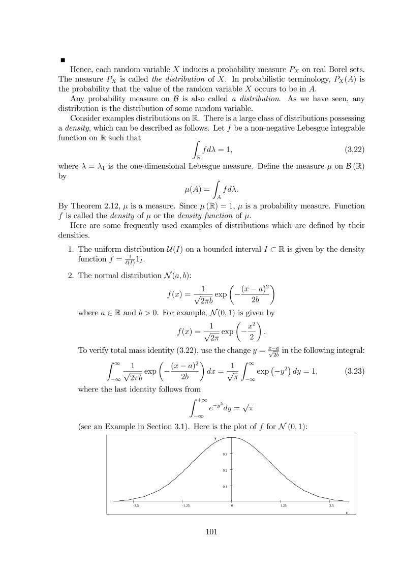
Hence, each random variable X induces a probability measure PX on real Borel sets.The measure PX is called the distribution of X. In probabilistic terminology, PX(A) isthe probability that the value of the random variable X occurs to be in A.Any probability measure on B is also called a distribution. As we have seen, any

distribution is the distribution of some random variable.Consider examples distributions on R. There is a large class of distributions possessing

a density, which can be described as follows. Let f be a non-negative Lebesgue integrablefunction on R such that Z

Rfdλ = 1, (3.22)

where λ = λ1 is the one-dimensional Lebesgue measure. Define the measure μ on B (R)by

μ(A) =

ZA

fdλ.

By Theorem 2.12, μ is a measure. Since μ (R) = 1, μ is a probability measure. Functionf is called the density of μ or the density function of μ.Here are some frequently used examples of distributions which are defined by their

densities.

1. The uniform distribution U(I) on a bounded interval I ⊂ R is given by the densityfunction f = 1

(I)1I .

2. The normal distribution N (a, b):

f(x) =1√2πb

exp

µ−(x− a)2

2b

¶where a ∈ R and b > 0. For example, N (0, 1) is given by

f(x) =1√2πexp

µ−x

2

2

¶.

To verify total mass identity (3.22), use the change y = x−a√2bin the following integral:Z ∞

−∞

1√2πb

exp

µ−(x− a)2

2b

¶dx =

1√π

Z ∞

−∞exp

¡−y2

¢dy = 1, (3.23)

where the last identity follows fromZ +∞

−∞e−y

2

dy =√π

(see an Example in Section 3.1). Here is the plot of f for N (0, 1):

2.51.250-1.25-2.5

0.3

0.2

0.1

x

y

x

y

101

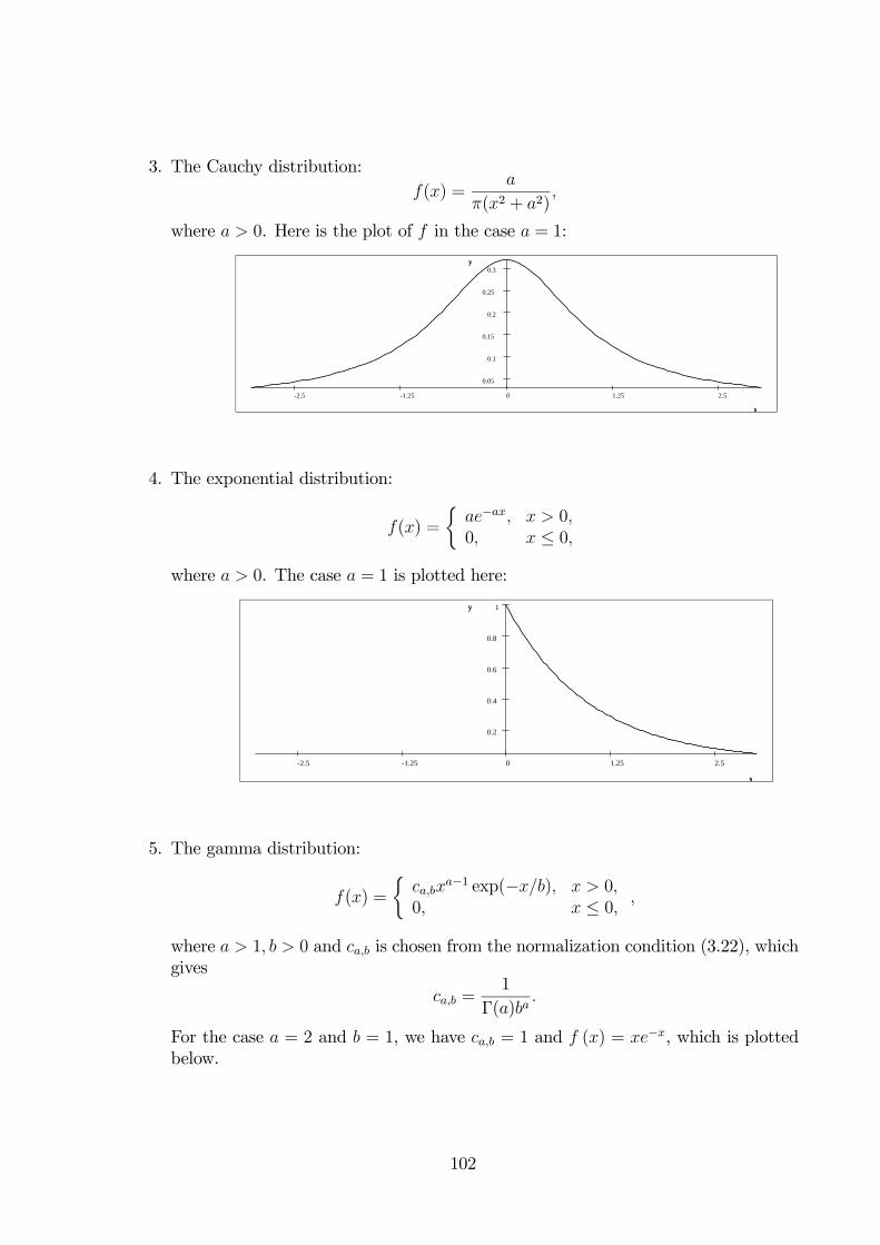
3. The Cauchy distribution:f(x) =

a

π(x2 + a2),

where a > 0. Here is the plot of f in the case a = 1:

2.51.250-1.25-2.5

0.3

0.25

0.2

0.15

0.1

0.05

x

y

x

y

4. The exponential distribution:

f(x) =

½ae−ax, x > 0,0, x ≤ 0,

where a > 0. The case a = 1 is plotted here:

2.51.250-1.25-2.5

1

0.8

0.6

0.4

0.2

x

y

x

y

5. The gamma distribution:

f(x) =

½ca,bx

a−1 exp(−x/b), x > 0,0, x ≤ 0, ,

where a > 1, b > 0 and ca,b is chosen from the normalization condition (3.22), whichgives

ca,b =1

Γ(a)ba.

For the case a = 2 and b = 1, we have ca,b = 1 and f (x) = xe−x, which is plottedbelow.

102

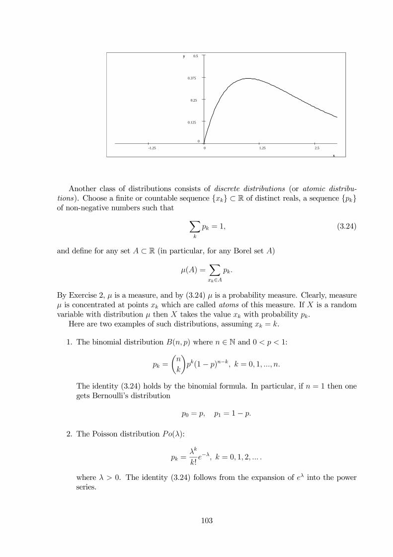
2.51.250-1.25

0.5

0.375

0.25

0.125

0

x

y

x

y

Another class of distributions consists of discrete distributions (or atomic distribu-tions). Choose a finite or countable sequence xk ⊂ R of distinct reals, a sequence pkof non-negative numbers such that X

k

pk = 1, (3.24)

and define for any set A ⊂ R (in particular, for any Borel set A)

μ(A) =Xxk∈A

pk.

By Exercise 2, μ is a measure, and by (3.24) μ is a probability measure. Clearly, measureμ is concentrated at points xk which are called atoms of this measure. If X is a randomvariable with distribution μ then X takes the value xk with probability pk.Here are two examples of such distributions, assuming xk = k.

1. The binomial distribution B(n, p) where n ∈ N and 0 < p < 1:

pk =

µn

k

¶pk(1− p)n−k, k = 0, 1, ..., n.

The identity (3.24) holds by the binomial formula. In particular, if n = 1 then onegets Bernoulli’s distribution

p0 = p, p1 = 1− p.

2. The Poisson distribution Po(λ):

pk =λk

k!e−λ, k = 0, 1, 2, ... .

where λ > 0. The identity (3.24) follows from the expansion of eλ into the powerseries.

103

3.3 Functionals of random variables

Definition. IfX is a random variable on a probability space (Ω,F ,P) then its expectationis defined by

E (X) =ZΩ

X(ω)dP(ω),

provided the integral in the right hand side exists (that is, either X is non-negative or Xis integrable, that is E (|X|) <∞).In other words, the notation E (X) is another (shorter) notation for the integralR

ΩXdP.By simple properties of Lebesgue integration and a probability measure, we have the

following properties of E:

1. E(X + Y ) = E (X) + E (Y ) provided all terms make sense;

2. E (αX) = αE (X) where α ∈ R;

3. E1 = 1.

4. infX ≤ EX ≤ supX.

5. |EX| ≤ E |X| .

Definition. If X is an integrable random variable then its variance is defined by

varX = E¡(X − c)2

¢, (3.25)

where c = E (X).The variance measures the quadratic mean deviation of X from its mean value c =

E (X). Another useful expression for variance is the following:

varX = E¡X2¢− (E (X))2 . (3.26)

Indeed, from (3.25), we obtain

varX = E¡X2¢− 2cE (X) + c2 = E

¡X2¢− 2c2 + c2 = E

¡X2¢− c2.

Since by (3.25) varX ≥ 0, it follows from (3.26) that

(E (X))2 ≤ E(X2). (3.27)

Alternatively, (3.27) follows from a more general Cauchy-Schwarz inequality: for any tworandom variables X and Y ,

(E (|XY |))2 ≤ E(X2)E(Y 2). (3.28)

The definition of expectation is convenient to prove the properties of E but no goodfor computation. For the latter, there is the following theorem.

104

Theorem 3.3 Let X be a random variable and f be a Borel function on (−∞,+∞).Then f(X) is also a random variable and

E(f(X)) =ZRf(x)dPX(x). (3.29)

If measure PX has the density g (x) then

E(f(X)) =ZRf(x)g (x) dλ (x) . (3.30)

Proof. Function f(X) is measurable by Theorem 2.2. It suffices to prove (3.29) fornon-negative f . Consider first an indicator function

f(x) = 1A(x),

for some Borel set A ⊂ R. For this function, the integral in (3.29) is equal toZA

dPX(A) = PX(A).

On the other hand,f(X) = 1A(X) = 1X∈A

and

E (f(X)) =ZΩ

1X∈AdP = P(X ∈ A) = PX(A).

Hence, (3.29) holds for the indicator functions. In the same way one proves (3.30) forindicator functions.By the linearity of the integral, (3.29) (and (3.30)) extends to functions which are finite

linear combinations of indicator functions. Then by the monotone convergence theoremthe identity (3.29) (and (3.30)) extends to infinite linear combinations of the indicatorfunctions, that is, to simple functions, and then to arbitrary Borel functions f .In particular, it follows from (3.29) and (3.30) that

E (X) =ZRx dPX(x) =

ZRxg (x) dλ (x) . (3.31)

Also, denoting c = E (X), we obtain

varX = E (X − c)2 =

ZR(x− c)2dPX =

ZR(x− c)2g (x) dλ (x) .

Example. If X ∼ N (a, b) then one finds

E (X) =Z +∞

−∞

x√2πb

exp

Ã−(x− a)2

2b

!dx =

Z +∞

−∞

y + a√2πb

exp

µ−y

2

2b

¶dy = a,

where we have used the fact thatZ +∞

−∞

y√2πb

exp

µ−y

2

2b

¶dy = 0

105

because the function under the integral is odd, andZ +∞

−∞

a√2πb

exp

µ−y

2

2b

¶dy = a,

which is true by (3.23). Similarly, we have

varX =

Z +∞

−∞

(x− a)2√2πb

exp

Ã−(x− a)2

2b

!dx =

Z +∞

−∞

y2√2πb

exp

µ−y

2

2b

¶dy = b, (3.32)

where the last identity holds by Exercise 50. Hence, for the normal distribution N (a, b),the expectation is a and the variance is b.

Example. If PX is a discrete distribution with atoms xk and values pk then (3.31)becomes

E (X) =∞Xk=0

xkpk.

For example, if X ∼ Po(λ) then one finds

E (X) =∞Xk=1

kλk

k!e−λ = λ

∞Xk=1

λk−1

(k − 1)!e−λ = λ.

Similarly, we have

E¡X2¢=

∞Xk=1

k2λk

k!e−λ =

∞Xk=1

(k − 1 + 1) λk

(k − 1)!e−λ

= λ2∞Xk=2

λk−2

(k − 2)!e−λ + λ

∞Xk=1

λk−1

(k − 1)!e−λ = λ2 + λ,

whencevarX = E

¡X2¢− (E (X))2 = λ.

Hence, for the Poisson distribution with the parameter λ, both the expectation and thevariance are equal to λ.

3.4 Random vectors and joint distributions

Definition. A mapping X : Ω → Rn is called a random vector (or a vector-valuedrandom variable) if it is measurable with respect to the σ-algebra F .Let X1, ..., Xn be the components of X. Recall that the measurability of X means

that the following set

ω ∈ Ω : X1 (ω) ≤ x1, ...,Xn (ω) ≤ xn (3.33)

is measurable for all reals x1, ..., xn.

Lemma 3.4 A mapping X : Ω→ Rn is a random vector if and only if all its componentsX1, ...,Xn are random variables.

106

Proof. If all components are measurable then all sets X1 ≤ x1 , ..., Xn ≤ xn aremeasurable and, hence, the set (3.33) is also measurable as their intersection. Conversely,let the set (3.33) is measurable for all xk. Since

X1 ≤ x =∞S

m=1

X1 ≤ x,X2 ≤ m,X3 ≤ m, ...,Xn ≤ m

we see that X1 ≤ x is measurable and, hence, X1 is a random variable. In the sameway one handles Xk with k > 1.

Corollary. If X : Ω→ Rn is a random vector and f : Rn → Rm is a Borel mapping thenf X : Ω→ Rm is a random vector.Proof. Let f1, ..., fm be the components of f . By the argument similar to Lemma

3.4, each fk is a Borel function on Rn. Since the components X1, ...,Xn are measurablefunctions, by Theorem 2.2 the function fk (X1, ...,Xn) is measurable, that is, a randomvariable. Hence, again by Lemma 3.4 the mapping f (X1, ...,Xn) is a random vector.As follows from Lemma 2.1, for any random vector X : Ω → Rn and for any Borel

set A ⊂ Rn, the set X ∈ A = X−1 (A) is measurable. Similarly to the one-dimensionalcase, introduce the distribution measure PX on B(Rn) by

PX(A) = P (X ∈ A) .

Lemma 3.5 If X is a random vector then PX is a probability measure on B(Rn). Con-versely, if μ is any probability measure on B(Rn) then there exists a random vector Xsuch that PX = μ.

The proof is the same as in the dimension 1 (see Lemma 3.2) and is omitted.If X1, ..., Xn is a sequence of random variable then consider the random vector X =

(X1, ...,Xn) and its distribution PX .

Definition. The measure PX is referred to as the joint distribution of the random vari-ables X1,X2, ...,Xn. It is also denoted by PX1X2...Xn .

As in the one-dimensional case, any non-negative measurable function g(x) on Rn suchthat Z

Rng(x)dx = 1,

is associated with a probability measure μ on B(Rn), which is defined by

μ(A) =

ZA

g(x)λn (x) .

The function g is called the density of μ. If the distribution PX of a random vector Xhas the density g then we also say that X has the density g (or the density function g).

Theorem 3.6 If X = (X1, ..., Xn) is a random vector and f : Rn → R is a Borel functionthen

Ef(X) =ZRn

f(x)dPX(x).

If X has the density g (x) then

Ef(X) =ZRn

f(x)g (x) dλn(x). (3.34)

107

The proof is exactly as that of Theorem 3.3 and is omitted.One can also write (3.34) in a more explicit form:

Ef(X1, X2, ...,Xn) =

ZRn

f(x1, ..., xn)g (x1, ..., xn) dλn(x1, ..., xn). (3.35)

As an example of application of Theorem 3.6, let us show how to recover the density of acomponent Xk given the density of X.

Corollary. If a random vector X has the density function g then its component X1 hasthe density function

g1(x) =

ZRn−1

g(x, x2, ..., xn) dλn−1 (x2, ..., xn) . (3.36)

Similar formulas take places for other components.Proof. Let us apply (3.35) with function f(x) = 1x1∈A where A is a Borel set on R;

that is,

f(x) =

½1, x1 ∈ A0, x1 /∈ A

= 1A×R×...×R .

ThenEf(X1, ...,Xn) = P (X1 ∈ A) = PX1(A),

and (3.35) together with Fubini’s theorem yield

PX1(A) =

ZRn1A×R×...×R (x1, ..., xn) g (x1, ..., xn) dλn (x1, ..., xn)

=

ZA×Rn−1

g (x1, ..., xn) dλn (x1, ..., xn)

=

ZA

µZRn−1

g (x1, ..., xn) dλn−1 (x2, ..., xn)

¶dλ1 (x1) .

This implies that the function in the brackets (which is a function of x1) is the density ofX1, which proves (3.36).

Example. Let X,Y be two random variables with the joint density function

g(x, y) =1

2πexp

µ−x

2 + y2

2

¶(3.37)

(the two-dimensional normal distribution). Then X has the density function

g1(x) =

Z +∞

−∞g(x, y)dy =

1√2πexp

µ−x

2

2

¶,

that is, X ∼ N (0, 1). In the same way Y ∼ N (0, 1).

Theorem 3.7 Let X : Ω → Rn be a random variable with the density function g. LetΦ : Rn → Rn be a diffeomorphism. Then the random variable Y = Φ (X) has the followingdensity function

h = g Φ−1¯det

¡Φ−1

¢0 ¯.

108

Proof. We have for any open set A ∈ Rn

P (Φ (X) ∈ A) = P¡X ∈ Φ−1 (A)

¢=

ZΦ−1(A)

g (x) dλn (x) .

Substituting x = Φ−1 (y) we obtain by Theorem 3.1ZΦ−1(A)

g (x) dλn (x) =

ZA

g¡Φ−1 (y)

¢ ¯det

¡Φ−1 (y)

¢0 ¯dλn (y) =

ZA

hdλn,

so that

P (Y ∈ A) =

ZA

hdλn. (3.38)

Since on the both sides of this identity we have finite measures on B (Rn) that coincideon open sets, it follows from the uniqueness part of the Carathéodory extension theoremthat the measures coincides on all Borel sets. Hence, (3.38) holds for all Borel sets A,which was to be proved.

Example. For any α ∈ R \ 0, the density function of Y = αX is

h (x) = g³xα

´|α|−n .

In particular, if X ∼ N (a, b) then αX ∼ N (αa, α2b) .As another example of application of Theorem 3.7, let us prove the following statement.

Corollary. Assuming that X,Y are two random variables with the joint density functiong (x, y). Then the random variable U = X + Y has the density function

h1 (u) =1

2

ZRg

µu+ v

2,u− v

2

¶dλ (v) =

ZRg (t, u− t) dt, (3.39)

and V = X − Y has the density function

h2 (v) =1

2

ZRg

µu+ v

2,u− v

2

¶dλ (u) =

ZRg (t, t− v) dt. (3.40)

Proof. Consider the mapping Φ : R2 → R2 is given by

Φ

µxy

¶=

µx+ yx− y

¶,

and the random vector µUV

¶=

µX + YX − Y

¶= Φ (X,Y ) .

Clearly, Φ is a diffeomorphism, and

Φ−1µ

uv

¶=

µu+v2

u−v2

¶,¡Φ−1

¢0=

µ1/2 1/21/2 −1/2

¶,¯det

¡Φ−1

¢0 ¯=1

2.

109

Therefore, the density function h of (U, V ) is given by

h (u, v) =1

2g

µu+ v

2,u− v

2

¶.

By Corollary to Theorem 3.6, the density function h1 of U is given by

h1 (u) =

ZRh (u, v) dλ (v) =

1

2

ZRg

µu+ v

2,u− v

2

¶dλ (v) .

The second identity in (3.39) is obtained using the substitution t = u+v2. In the same way

one proves (3.40).

Example. Let X,Y be again random vectors with joint density (3.37). Then by (3.39)we obtain the density of X + Y :

h1 (u) =1

2

Z ∞

−∞

1

2πexp

Ã−(u+ v)2 + (u− v)2

8

!dv

=1

4π

Z ∞

−∞exp

µ−u

2

4− v2

4

¶dv

=1√4π

e−14u2 .

Hence, X + Y ∼ N (0, 2) and in the same way X − Y ∼ N (0, 2).

3.5 Independent random variables

Let (Ω,F ,P) be a probability space as before.Definition. Two random vectors X : Ω→ Rn and Y : Ω→ Rm are called independent if,for all Borel sets A ∈ Bn and B ∈ Bm, the events X ∈ A and Y ∈ B are independent,that is

P (X ∈ A and Y ∈ B) = P(X ∈ A)P(Y ∈ B).

Similarly, a sequence Xi of random vectors Xi : Ω → Rni is called independent if, forany sequence Ai of Borel sets Ai ∈ Bni, the events Xi ∈ Ai are independent. Herethe index i runs in any index set (which may be finite, countable, or even uncountable).

If X1, ...,Xk is a finite sequence of random vectors, such that Xi : Ω → Rni then wecan form a vector X = (X1, ..., Xk) whose components are those of all Xi; that is, X is ann-dimensional random vector where n = n1+ ...+nk. The distribution measure PX of Xis called the joint distribution of the sequence X1, ..., Xk and is also denoted by PX1...Xk

.A particular case of the notion of a joint distribution for the case when all Xi are

random variables, was considered above.

Theorem 3.8 Let Xi be a ni-dimensional random vector, i = 1, ..., k. The sequenceX1,X2, ..., Xk is independent if and only if their joint distribution PX1...Xk

coincides withthe product measure of PX1 , PX2, ..., PXk

, that is

PX1...Xk= PX1 × ...× PXk

. (3.41)

110

If X1,X2, ..., Xk are independent and in addition Xi has the density function fi(x) thenthe sequence X1, ...,Xk has the joint density function

f(x) = f1(x1)f2(x2)...fk(xk),

where xi ∈ Rni and x = (x1, ..., xk) ∈ Rn.

Proof. If (3.41) holds then, for any sequence Aiki=1 of Borel sets Ai ⊂ Rni, considertheir product

A = A1 ×A2 × ...×Ak ⊂ Rn (3.42)

and observe that

P (X1 ∈ A1, ..., Xk ∈ Ak) = P (X ∈ A)

= PX (A)

= PX1 × ...× PXk(A1 × ...×Ak)

= PX1 (A1) ...PXk(Ak)

= P (X1 ∈ A1) ...P (Xk ∈ Ak) .

Hence, X1, ...,Xk are independent.Conversely, ifX1, ...,Xk are independent then, for any set A of the product form (3.42),

we obtain

PX (A) = P (X ∈ A)

= P (X1 ∈ A1, X2 ∈ A2, ..., Xk ∈ Ak)

= P (X1 ∈ A1 )P(X2 ∈ A2)...P(Xk ∈ Ak)

= PX1 × ...× PXk(A) .

Hence, the measure PX and the product measure PX1× ...×PXkcoincide on the sets of the

form (3.42). Since Bn is the minimal σ-algebra containing the sets (3.42), the uniquenesspart of the Carathéodory extension theorem implies that these two measures coincide onBn, which was to be proved.To prove the second claim, observe that, for any set A of the form (3.42), we have by

Fubini’s theorem

PX (A) = PX1 (A1) ...PXk(Ak)

=

ZA1

f1 (x1) dλn1 (x1) ...

ZAk

fk (xk) dλnk (xk)

=

ZA1×...×Ak

f1 (x1) ...fk (xk) dλn (x)

=

ZA

f (x) dλn (x) ,

where x = (x1, ..., xk) ∈ Rn. Hence, the two measures PX (A) and

μ (A) =

ZA

f (x) dλn (x)

111

coincide of the product sets, which implies by the uniqueness part of the Carathéodoryextension theorem that they coincide on all Borel sets A ⊂ Rn.

Corollary. If X and Y are independent integrable random variables then

E(XY ) = E (X)E (Y ) (3.43)

andvar(X + Y ) = varX + varY. (3.44)

Proof. Using Theorems 3.6, 3.8, and Fubini’s theorem, we have

E(XY ) =

ZR2xydPXY =

ZR2xyd (PX × PY ) =

µZRxdPX

¶µZRydPY

¶= E(X)E(Y ).

To prove the second claim, observe that var (X + c) = varX for any constant c. Hence,we can assume that E (X) = E (Y ) = 0. In this case, we have varX = E (X2). Using(3.43) we obtain

var(X + Y ) = E(X + Y )2 = E¡X2¢+ 2E(XY ) + E

¡Y 2¢= EX2 + EY 2 = varX + varY.

The identities (3.43) and (3.44) extend to the case of an arbitrary finite sequence ofindependent integrable random variables X1, ...,Xn as follows:

E (X1...Xn) = E (X1) ...E (Xn) ,

var (X1 + ...+Xn) = varX1 + ...+ varXn ,

and the proofs are the same.

Example. Let X,Y be independent random variables and

X ∼ N (a, b) , Y ∼ N (a0, b0) .

Let us show thatX + Y ∼ N (a+ a0, b+ b0) .

Let us first simply evaluate the expectation and the variance of X + Y :

E (X + Y ) = E (X) + E (Y ) = a+ a0,

and, using the independence of X,Y and (3.44),

var (X + Y ) = var (X) + var (Y ) = b+ b0.

However, this does not yet give the distribution of X + Y . To simplify the furtherargument, rename X − a to X, Y − a0 to Y , so that we can assume in the sequel thata = a0 = 0. Also for simplicity of notation, set c = b0. By Theorem 3.8, the joint densityfunction of X,Y is as follows:

g (x, y) =1√2πb

exp

µ−x

2

2b

¶1√2πc

exp

µ−y

2

2c

¶=

1

2π√bcexp

µ−x

2

2b− y2

2c

¶.

112

By Corollary to Theorem 3.7, we obtain that the random variable U = X + Y has thedensity function

h (u) =

ZRg (t, u− t) dλ (t)

=

Z ∞

−∞

1

2π√bcexp

Ã− t2

2b− (u− t)2

2c

!dt

=

Z ∞

−∞

1

2π√bcexp

µ−µ1

b+1

c

¶t2

2+

ut

c− u2

2c

¶dt.

Next compute Z +∞

−∞exp

¡−αt2 + 2βt

¢dt

where α > 0 and β ∈ R. We have

−αt2 + 2βt = −αµt2 − 2β

αt+

β2

α2− β2

α2

¶= −α

µt− β

α

¶2+

β2

α.

Hence, substituting√α¡t− β

α

¢= s, we obtainZ +∞

−∞exp

¡−αt2 + 2βt

¢dt =

eβ2/α

√α

Z ∞

−∞exp

¡−s2

¢ds =

rπ

αeβ

2/α.

Setting here α = 12

¡1b+ 1

c

¢and β = u

2c, we obtain

h (u) =1

2π√bce−u

2/(2c)

r2bcπ

b+ ceu2

4c22bcb+c =

1p2π (b+ c)

exp

µ− u2

2 (b+ c)

¶,

that is, U ∼ N (0, b+ c).

Example. Consider a sequence Xini=1 of independent Bernoulli variables taking 1 withprobability p, and 0 with probability 1− p, where 0 < p < 1. Set S = X1 + ...+Xn andprove that, for any k = 0, 1, ..., n

P (S = k) =

µn

k

¶pk(1− p)n−k. (3.45)

Indeed, the sum S is equal to k if and only if exactly k of the values X1, ..., Xn are equalto 1 and n − k are equal to 0. The probability, that the given k variables from Xi, sayXi1 , ...,Xik are equal to 1 and the rest are equal to 0, is equal to pk (1− p)n−k. Sincethe sequence (i1, ..., ik) can be chosen in

¡nk

¢ways, we obtain (3.45). Hence, S has the

binomial distribution B(n, p). This can be used to obtain in an easy way the expectationand the variance of the binomial distribution — see Exercise 67d.

In the next statement, we collect some more useful properties of independent randomvariables.

113

Theorem 3.9 (a) If Xi : Ω → Rni is a sequence of independent random vectors andfi : Rni → Rmi is a sequence of Borel functions then the random vectors fi(Xi) areindependent.(b) If X1, X2, ..., Xn, Y1, Y2, .., Ym is a sequence of independent random variables then

the random vectors

X = (X1, X2, ..., Xn) and Y = (Y1, Y2, ..., Ym)

are independent.(c) Under conditions of (b), for all Borel functions f : Rn → R and g : Rm → R, the

random variables f (X1, ..., Xn) and g (Y1, ..., Ym) are independent.

Proof. (a) Let Ai be a sequence of Borel sets, Ai ∈ Bmi. We need to show that theevents fi (Xi) ∈ Ai are independent. Since

fi (Xi) ∈ Ai =©Xi ∈ f−1i (Ai)

ª= Xi ∈ Bi ,

where Bi = f−1 (Ai) ∈ Bni, these sets are independent by the definition of the indepen-dence of Xi.(b) We have by Theorem 3.8

PXY = PX1 × ...× PXn × PY1 × ...× PYm

= PX × PY .

Hence, X and Y are independent.(c) The claim is an obvious combination of (a) and (b) .

3.6 Sequences of random variables

Let Xi∞i=1 be a sequence of independent random variables and consider their partialsums

Sn = X1 +X2 + ...+Xn.

We will be interested in the behavior of Sn as n→∞. The necessity of such considerationsarises in many mathematical models of random phenomena.

Example. Consider a sequence on n independent trials of coin tossing and set Xi = 1if at the i-th tossing the coin lands showing heads, and Xi = 0 if the coin lands showingtails. Assuming that the heads appear with probability p, we see each Xi has the sameBernoulli distribution: P (Xi = 1) = p and P (Xi = 0) = 1− p. Based on the experience,we can assume that the sequence Xi is independent. Then Sn is exactly the number ofheads in a series of n trials. If n is big enough then one can expect that Sn ≈ np. Theclaims that justify this conjecture are called laws of large numbers. Two such statementsof this kind will be presented below.As we have seen in Section 1.10, for any positive integer n, there exist n independent

events with prescribed probabilities. Taking their indicators, we obtain n independentBernoulli random variables. However, in order to make the above consideration of infinitesequences of independent random variables meaningful, one has to make sure that suchsequences do exist. The next theorem ensures that, providing enough supply of sequencesof independent random variables.

114

Theorem 3.10 Let μii∈I be a family of probability measures on B (R) where I is anarbitrary index set. Then there exists a probability space (Ω,F ,P) and a family Xii∈Iof independent random variables on Ω such that PXi = μi.

The space Ω is constructed as the (infinite) product RI and the probability measure Pon Ω is constructed as the product

Ni∈I μi of the measures μi. The argument is similar

to Theorem 2.22 but technically more involved. The proof is omitted.Theorem 3.10 is a particular case of a more general Kolmogorov’s extension theorem

that allows constructing families of random variables with prescribed joint densities.

3.7 The weak law of large numbers

Definition. We say that a sequence Yn of random variables converges in probability toa random variable Y and write Yn

P−→ Y if, for any ε > 0,

limn→∞

P (|Yn − Y | > ε) = 0.

This is a particular case of the convergence in measure — see Exercise 41.

Theorem 3.11 (The weak law of large numbers) Let Xi∞i=1 be independent sequenceof random variables having a common finite expectation E (Xi) = a and a common finitevariance varXi = b. Then

Snn

P−→ a. (3.46)

Hence, for any ε > 0,

Pµ¯

Snn− a

¯≤ ε

¶→ 1 as n→∞

which means that, for large enough n, the average Sn/n concentrates around a with aprobability close to 1.

Example. In the case of coin tossing, a = E (Xi) = p and varXi is finite so that Snn

P−→ p.One sees that in some sense Sn/n ≈ p, and the precise meaning of that is the following:

Pµ¯

Snn− p

¯≤ ε

¶→ 1 as n→∞.

Example. Assume that all Xi ∼ N (0, 1). Using the properties of the sums of indepen-dent random variables with the normal distribution, we obtain

Sn ∼ N (0, n)

andSnn∼ N

µ0,1

n

¶.

115

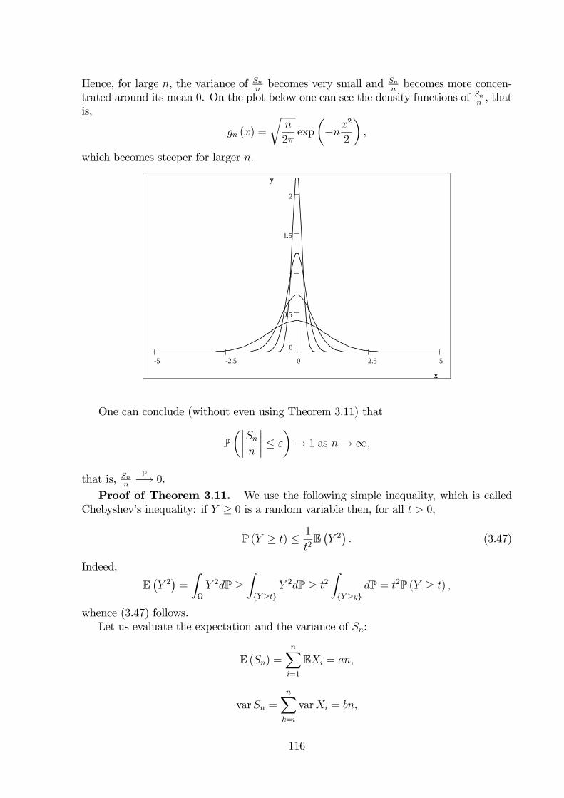
Hence, for large n, the variance of Snnbecomes very small and Sn

nbecomes more concen-

trated around its mean 0. On the plot below one can see the density functions of Snn, that

is,

gn (x) =

rn

2πexp

µ−nx

2

2

¶,

which becomes steeper for larger n.

52.50-2.5-5

2

1.5

1

0.5

0

x

y

x

y

One can conclude (without even using Theorem 3.11) that

Pµ¯

Snn

¯≤ ε

¶→ 1 as n→∞,

that is, Snn

P−→ 0.

Proof of Theorem 3.11. We use the following simple inequality, which is calledChebyshev’s inequality: if Y ≥ 0 is a random variable then, for all t > 0,

P (Y ≥ t) ≤ 1

t2E¡Y 2¢. (3.47)

Indeed,

E¡Y 2¢=

ZΩ

Y 2dP ≥ZY≥t

Y 2dP ≥ t2ZY≥y

dP = t2P (Y ≥ t) ,

whence (3.47) follows.Let us evaluate the expectation and the variance of Sn:

E (Sn) =nXi=1

EXi = an,

varSn =nXk=i

varXi = bn,

116

where in the second line we have used the independence of Xi and Corollary to Theorem3.8. Hence, applying (3.47) with Y = |Sn − an|, we obtain

P (|Sn − an| ≥ εn) ≤ 1

(εn)2E (Sn − an)2 =

varSn

(εn)2=

bn

(εn)2=

b

ε2n.

Therefore,

Pµ¯

Snn− a

¯≥ ε

¶≤ b

ε2n, (3.48)

whence (3.46) follows.

3.8 The strong law of large numbers

In this section we use the convergence of random variables almost surely (a.s.) Namely, ifXn∞n=1 is a sequence of random variables then we say that Xn converges to X a.s. andwrite Xn

a.s.−→ X if Xn → X almost everywhere, that is,

P (Xn → X) = 1.

In the expanded form, this means that

P³n

ω : limn→∞

Xn (ω) = X (ω)o´

= 1.

To understand the difference between the convergence a.s. and the convergence inprobability, consider an example.

Example. Let us show an example where XnP−→ X but Xn does not converges to X

a.s. Let Ω = [0, 1], F = B ([0, 1]), and P = λ1. Let An be an interval in [0, 1] and set

Xn = 1An . Observe that if (An)→ 0 then XnP−→ 0 because for all ε ∈ (0, 1)

P (Xn > ε) = P (Xn = 1) = (An) .

However, for certain choices of An, we do not have Xna.s.−→ 0. Indeed, one can construct

An so that (An)→ 0 but nevertheless any point ω ∈ [0, 1] is covered by these intervalsinfinitely many times. For example, one can take as An the following sequence:

[0, 1] ,£0, 1

2

¤,£12, 1¤,£

0, 13

¤,£13, 23

¤,£23, 1¤,£

0, 14

¤,£14, 24

¤,£24, 34

¤,£34, 1¤

...

For any ω ∈ [0, 1], the sequence Xn(ω) contains the value 1 infinitely many times, whichmeans that this sequence does not converge to 0. It follows that Xn does not converge to0 a.s.; moreover, we have P (Xn → 0) = 0.

The following theorem states the relations between the two types of convergence.

117

Theorem 3.12 Let Xn be a sequence of random variables.

(a) If Xna.s.−→ X then Xn

P−→ X (hence, the convergence a.s. is stronger than theconvergence in probability).(b) If, for any ε > 0,

∞Xn=1

P (|Xn −X| > ε) <∞ (3.49)

then Xna.s.−→ X.

(c) If XnP−→ X then there exists a subsequence Xnk

a.s.−→ X.

The proof of Theorem 3.12 is contained in Exercise 42. In fact, we need only part (b) ofthis theorem. The condition (3.49) is called the Borel-Cantelli condition. It is obviously

stronger that XnP−→ X because the convergence of a series implies that the terms of

the series go to 0. Part (b) says that the Borel-Cantelli condition is also stronger thanXn

a.s.−→ X, which is not that obvious.Let Xi be a sequence of random variables. We say that this sequence is identically

distributed if allXi have the same distribution measure. If Xi are identically distributedthen their expectations are the same and the variances are the same.As before, set Sn = X1 + ...+Xn.

Theorem 3.13 (The strong law of large numbers) Let Xi∞i=1 be a sequence of indepen-dent identically distributed random variables with a finite expectation E (Xi) = a and afinite variance varXi = b. Then

Snn

a.s.−→ a. (3.50)

The word “strong” is the title of the theorem refers to the convergence a.s. in (3.50),as opposed to the weaker convergence in probability in Theorem 3.11 (cf. (3.46)).The statement of Theorem 3.13 remains true if one drops the assumption of the finite-

ness of varXn. Moreover, the finiteness of the mean E (Xn) is not only sufficient but alsonecessary condition for the existence of the limit lim sn

na.s. (Kolmogorov’s theorem). An-

other possibility to relax the hypotheses is to drop the assumption that Xn are identicallydistributed but still require that Xn have a common finite mean and a common finitevariance. The proofs of these stronger results are much longer and will not be presentedhere.Proof of Theorem 3.13. By Theorem 3.12(b), it suffices to verify the Borel-Cantelli

condition, that is, for any ε > 0,∞Xn=1

Pµ¯

Snn− a

¯> ε

¶<∞. (3.51)

In the proof of Theorem 3.11, we have obtained the estimate

Pµ¯

Snn− a

¯≥ ε

¶≤ b

ε2n, (3.52)

which however is not enough to prove (3.51), because∞Xn=1

1

n=∞.

118

Nevertheless, taking in (3.52) n to be a perfect square k2, where k ∈ N, we obtain∞Xk=1

Pµ¯

Sk2

k2− a

¯> ε

¶≤

∞Xk=1

b

ε2k2<∞,

whence by Theorem 3.12(b)Sk2

k2a.s.−→ a. (3.53)

Now we will extend this convergence to the whole sequence Sn, that is, fill gaps betweenthe perfect squares. This will be done under the assumption that all Xi are non-negative(the general case of a signed Xi will be treated afterwards). In this case the sequence Snis increasing. For any positive integer n, find k so that

k2 ≤ n < (k + 1)2. (3.54)

Using the monotonicity of Sn and (3.54), we obtain

Sk2

(k + 1)2≤ Sn

n≤

S(k+1)2

k2.

Since k2 ∼ (k + 1)2 as k →∞, it follows from (3.53) that

Sk2

(k + 1)2a.s.−→ a and

S(k+1)2

k2a.s.−→ a ,

whence we conclude thatSnn

a.s.−→ a.

Note that in this argument we have not used the hypothesis that Xi are identicallydistributed. As in the proof of Theorem 3.11, we only have used that Xi are independentrandom variables and that the have a finite common expectation a and a finite commonvariance.Now we get rid of the restriction Xi ≥ 0. For a signed Xi, consider the positive X+

i

part and the negative parts X−i . Then the random variables X

+i are independent because

we can write X+i = f(Xi) where f (x) = x+, and apply Theorem 3.9. Next, X+

i has finiteexpectation and variance by X+ ≤ |X|. Furthermore, by Theorem 3.3 we have

E¡X+

i

¢= E (f (Xi)) =

ZRf (x) dPXi

.

Since all measures PXi are the same, it follows that all the expectations E¡X+

i

¢are the

same; seta+ := E

¡X+

i

¢.

In the same way, the variances varX+i are the same. Setting

S+n = X+1 +X+

2 + ...+X+n ,

we obtain by the first part of the proof that

S+nn

a.s.−→ a+ as n→∞.

119

In the same way, considering X−i and setting a

− = E¡X−

i

¢and

S−n = X−1 + ...+X−

n ,

we obtainS−nn

a.s.−→ a− as n→∞.

Subtracting the two relations and using that

S+n − S−n = Sn

anda+ − a− = E

¡X+

i

¢− E

¡X−

i

¢= E (Xi) = a,

we obtainSnn

a.s.−→ a as n→∞,

which finishes the proof.

120

3.9 Extra material: the proof of the Weierstrass theorem usingthe weak law of large numbers

Here we show an example how the weak law of large numbers allows to prove the followingpurely analytic theorem.

Theorem 3.14 (TheWeierstrass theorem) Let f (x) be a continuous function on a boundedinterval [a, b]. Then, for any ε > 0, there exists a polynomial P (x) such that

supx∈[a,b]

|f(x)− P (x)| < ε.

Proof. It suffices to consider the case of the interval [0, 1]. Consider a sequence Xi∞i=1of independent Bernoulli variables taking 1 with probability p, and 0 with probability 1−p,and set as before Sn = X1 + ...+Xn. Then, for k = 0, 1, ..., n,

P (Sn = k) =

µn

k

¶pk(1− p)n−k,

which implies

EfµSnn

¶=

nXk=0

f(k

n)P(Sn = k) =

nXk=0

f(k

n)

µn

k

¶pk (1− p)n−k .

The right hand side here can be considered as a polynomial in p. Denote

Bn(p) =nX

k=0

f(k

n)

µn

k

¶pk (1− p)n−k . (3.55)

The polynomial Bn(p) is called the Bernstein’s polynomial of f . It turns out to be a goodapproximation for f . The idea is that Sn/n converges in some sense to p. Therefore, wemay expect that Ef(Sn

n) converges to f(p). In fact, we will show that

limn→∞

supp∈[0,1]

|f(p)−Bn(p)| = 0, (3.56)

which will prove the claim of the theorem.First observe that f is uniformly continuous so that for any δ > 0 there exists ε =

ε(δ) > 0 such that if |x− y| ≤ ε then |f(x)− f(y)| ≤ δ. Using the binomial theorem, weobtain

1 = (p+ (1− p))n =nX

k=0

µn

k

¶pk (1− p)n−k ,

whence

f(p) =nX

k=0

f(p)

µn

k

¶pk (1− p)n−k .

Comparing with (3.55), we obtain

|f(p)−Bn(p)| ≤nX

k=0

¯f(p)− f(

k

n)

¯ µn

k

¶pk (1− p)n−k

=

⎛⎜⎝ X| kn−p|≤ε

+X| kn−p|>ε

⎞⎟⎠ ¯f(p)− f(k

n)

¯ µn

k

¶pk (1− p)n−k .

121

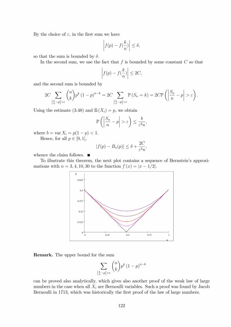
By the choice of ε, in the first sum we have¯f(p)− f(

k

n)

¯≤ δ,

so that the sum is bounded by δ.In the second sum, we use the fact that f is bounded by some constant C so that¯

f(p)− f(k

n)

¯≤ 2C,

and the second sum is bounded by

2CX| kn−p|>ε

µn

k

¶pk (1− p)n−k = 2C

X| kn−p|>ε

P (Sn = k) = 2CPµ¯

Snn− p

¯> ε

¶.

Using the estimate (3.48) and E (Xi) = p, we obtain

Pµ¯

Snn− p

¯> ε

¶≤ b

ε2n,

where b = varXi = p(1− p) < 1.Hence, for all p ∈ [0, 1],

|f(p)−Bn(p)| ≤ δ +2C

ε2n,

whence the claim follows.To illustrate this theorem, the next plot contains a sequence of Bernstein’s approxi-

mations with n = 3, 4, 10, 30 to the function f (x) = |x− 1/2|.

10.750.50.250

0.625

0.5

0.375

0.25

0.125

0

x

y

x

y

Remark. The upper bound for the sumX| kn−p|>ε

µn

k

¶pk (1− p)n−k

can be proved also analytically, which gives also another proof of the weak law of largenumbers in the case when all Xi are Bernoulli variables. Such a proof was found by JacobBernoulli in 1713, which was historically the first proof of the law of large numbers.

122