arX

iv:1

911.

0023

5v2

[as

tro-

ph.S

R]

12

May

202

0Mon. Not. R. Astron. Soc. 000, 1–16 () Printed 13 May 2020 (MN LATEX style file v2.2)

Mean field dynamo action in shear flows. I: fixed kinetic

helicity

Naveen Jingade1,2⋆ and Nishant K. Singh3,4†1Indian Institute of Science, Bangalore 560 012, India2Raman Research Institute, Sadashivanagar, Bangalore 560 080, India3Max Planck Institute for Solar System Research, Justus-von-Liebig-Weg 3, D-37077 Gottingen, Germany4Inter-University Centre for Astronomy and Astrophysics, Post Bag 4, Ganeshkhind, Pune 411 007, India

13 May 2020

ABSTRACT

We study mean-field dynamo action in a background linear shear flow by employ-ing pulsed renewing flows with fixed kinetic helicity and nonzero correlation time(τ). We use plane shearing waves in terms of time-dependent exact solutions to theNavier-Stokes equation as derived by Singh & Sridhar (2017). This allows us to self-consistently include the anisotropic effects of shear on the stochastic flow. We deter-mine the average response tensor governing the evolution of mean magnetic field, andstudy the properties of its eigenvalues which yield the growth rate (γ) and the cycleperiod (Pcyc) of the mean magnetic field. Non-axisymmetric mode of the mean-fielddecay as t → ∞ and hence are deemed unimportant for mean-field dynamo. Both, γand the wavenumber corresponding to the fastest growing axisymmetric mode varynon-monotonically with shear rate S when τ is comparable to the eddy turnover timeT , in which case, we also find quenching of dynamo when shear becomes too strong.When τ/T ∼ O(1), the cycle period (Pcyc) of growing dynamo wave scales with shearas Pcyc ∝ |S|−1 at small shear, and it becomes nearly independent of shear as shearbecomes too strong. This asymptotic behaviour at weak and strong shear has im-plications for magnetic activity cycles of stars in recent observations. Our study thusessentially generalizes the standard αΩ (or α2Ω) dynamo as also the α effect is affectedby shear and the modelled random flow has a finite memory.

Key words: dynamo - magnetic fields - MHD - turbulence - shear flows

1 INTRODUCTION

Coherent large-scale magnetic fields and mean differential rotation are two common features of most astrophysical objects, such

as, the Sun, stars, galaxies, etc (Parker 1979; Zeldovich et al. 1983; Ruzmaikin, Shukurov & Sokoloff 1998; Jones 2011; Han

2017). Magnetic fields in these systems are maintained by turbulent dynamo action where the standard paradigm for large-scale

component involves amplification of weak seed fields due to helical turbulence in shear flows (Moffatt 1978; Krause & Radler

1980; Brandenburg & Subramanian 2005). The α effect, which, in idealized settings, is a measure of net kinetic helicity and

arises naturally in systems with rotation and stratification, plays a crucial role in driving large scale dynamos in a variety

of systems (e.g. Dormy & Soward 2007; Charbonneau 2010; Brandenburg et al. 2012); see also Courvoisier, Hughes & Tobias

(2006); Hori & Yoshida (2008) for a more general description of the α effect, where non-local and non-instantaneous effect are

considered in the expression of turbulent EMF by employing integral relation between EMF and mean-field, unlike simplified

standard dynamo models where the EMF depends on the local and instantaneous value of the mean magnetic field.

Direct numerical simulations in galactic or solar contexts have shown that the large scale magnetic fields are naturally pro-

duced as a result of a mean-field turbulent dynamo in local as well as global setups, where the mirror symmetry of turbulence is

⋆ E-mail: naveen@rri.res.in† E-mail: nishant@iucaa.in

c© RAS

2 Jingade & Singh

broken either by having a helical driving or by enabling convection in a rotating system (Brandenburg, Bigazzi & Subramanian

2001; Gressel et al. 2008; Kapyla et al. 2012; Warnecke et al. 2014; Kapyla et al. 2016, 2018). Mean shear is common to these

studies and the dynamo is thought to be of αΩ-type, or, more generally, of α2Ω-type as the role of α-term in the generation of

shear-wise component may indeed be comparable to the Ω-effect (Viviani et al. 2019); see, e.g., Brandenburg & Subramanian

(2005), for different types of dynamos. It is known that the α-effect is a more complicated tensorial object (Radler et al. 2003;

Brandenburg & Subramanian 2005), which might be much different from the net kinetic helicity of the flow (Kleeorin & Rogachevskii

2003; Chamandy & Singh 2017). Turbulent transport coefficients, such as the α-tensor, are often numerically determined in

a variety of contexts (Sur et al. 2008; Mitra et al. 2009).

Somewhat less common approach to study the large-scale dynamo is to directly solve for the evolution of mean magnetic

field by determining the response function for a given smooth random flow (Gilbert & Bayly 1992; Kolekar, Subramanian & Sridhar

2012). Such a model is shown to faithfully represent a fast or small-scale dynamo (Zeldovich et al. 1984; Bayly & Childress

1988; Gilbert & Bayly 1992). Essentially all astrophysical bodies are expected to host a small-scale dynamo, which appears to

be always excited when the magnetic Reynolds number exceeds a critical value (Zeldovich et al. 1983). There are concerns that

its presence makes the description of large-scale dynamo in terms of standard mean field magnetohydrodynamics (MHD), or,

say, α-prescription, less straightforward (e.g. Schekochihin, Boldyrev & Kulsrud 2002; Courvoisier, Hughes & Tobias 2006).

Gilbert & Bayly (1992), hereafter GB92, chose random helical flows in their model where they also included the memory

effects, and showed analytically that the magnetic field develops intermittency in time1. They also found growing solutions

for the first moment or the mean magnetic field, and, in the limit of small correlation times, they recovered the predictions

of standard α2 dynamo for the growth rate. Kolekar, Subramanian & Sridhar (2012), hereafter KSS12, extended the work of

GB92 to also include the effect of shear, and showed quite generally, that the mean field dynamo action is not possible so

long as the flows are strictly non-helical. By considering a particular model of random helical flow, they derived a generalized

response tensor, which yields, for fixed kinetic helicity and small correlation times, the same dispersion relation as that from

a standard α2Ω dynamo. In paper II (Jingade & Singh 2020) we consider flows with fluctuating kinetic helicity, which has a

renovation time greater than the velocity renovation time, and show that the growth of mean-magnetic field is possible even

in the absence of negative turbulent diffusion (Kraichnan 1976a).

Following GB92; KSS12, we adopt here a renovating flow based model which allows us to describe the evolution of mean

magnetic field, without explicitly deriving any mean electromotive force (EMF) which is essential in standard mean field

MHD. In this model, one assumes an exactly solvable flow field in terms of a single plane wave which renovates itself after

each time interval τ . Thus, the time is split into equal intervals of length τ and the velocity fields in different intervals are

assumed to be statistically independent. The evolution of magnetic field is then determined by the realization of the velocity

field only in a fixed interval. Such a model neither involves any closure approximation, nor is it limited to low fluid or magnetic

Reynolds numbers. KSS12 in their analysis considered forced overdamped shearing waves to model the renovating flows. Here

we make use of plane shearing waves, which are time-dependent exact solutions to the Navier-Stokes equations as derived by

Singh & Sridhar (2017). Shear induces anisotropy in the renovating flow, which, in this work, is allowed to freely decay for

the renovation time τ , and it is resetted to the same amplitude at the beginning of each renovation interval. Such a resetting

essentially tries to capture the effects of a random forcing after every τ .

In Section 2 we present the model of renovating flow in a background linear shear flow and then discuss the helical shearing

waves which are used in this work. Linear shear makes the induction equation inhomogeneous in the lab frame; see Eq. (9).

To deal with this, we make use of shearing coordinate transformation and then determine the Cauchy’s solution for ideal

induction equation in shearing frame. We then derive an expression for the average response tensor governing the evolution

of mean magnetic field in Fourier space after suitably averaging over randomness of the flow. Behaviour of non-axisymmetric

modes of mean magnetic field is presented in Section 3. In Section 4 we present our findings on the axisymmetric mean field

dynamos, where we explore various properties of dynamo growth rate and its cycle period in detail, and discuss the significance

of new predictions from our model in light of recent observations. We conclude in Section 5.

2 MODEL DESCRIPTION

We, now investigate the evolution of the mean-magnetic field in the background shear flow along with the turbulence. Such

systems are common in astrophysical scenario like Sun, Galaxies, accretion disk etc. Let (e1,e2,e3) be the orthonormal

unit vectors in the Cartesian coordinate system in the lab frame, where X = (X1, X2, X3) is a position vector. We choose

mean shear to be acting in the e2 direction (azimuthal direction), varying along X1 linearly, which is a local shearing–sheet

1 The term ‘memory effect’ is used in this work to indicate that the random flow has non-zero correlation times. As clarified inSridhar & Singh (2014), this is equivalent to more usual notion of memory effects in dynamo theory when the turbulent EMF is affectedby the time dependence of the mean magnetic field, whereas in the white-noise case, the generalized EMF with a history term througha time-integral reduces to a simple expression leading to an instantaneous relation with the mean magnetic field.

c© RAS, MNRAS 000, 1–16

Mean field dynamo action in shear flows 3

approximation to the differential rotation of the disks (Goldreich & Lynden-Bell 1965; Brandenburg et al. 2008). The model

velocity field U can be written as, U(X , t) = S X1e2 + u(X, t), where u is the turbulent velocity field, and the shear rate S

is a constant parameter.

2.1 Renewing flows in shearing background

Let us consider the inviscid Navier–Stokes equation in the background linear shear flow for the unit mass density,(∂

∂t+ SX1

∂

∂X2

)u+ Su1e2 + (u·∇)u = −∇p , with ∇·u = 0, (1)

where we have also assumed the flow u to be incompressible. We look for the single helical wave solution of the form,

u(X, t) = A(St, q) sin(Q(t)·X +Ψ) + hC(St, q) cos(Q(t)·X +Ψ) (2)

where Q(t) is a shearing wavevector having the form Q = (q1 − Sq2(t− t0), q2, q3), q = (q1, q2, q3) is the wavevector at initial

time t0, and Ψ denotes the phase of the wave. This particular form of wave vector arises because of the inhomogeneity of the

Eq. (1) in the variable X1. A(St, q) and C(St, q) are the amplitudes of the sheared helical wave and h controls the relative

helicity of the flow. The above velocity field is supplemented by

Q(t)·A(t) = 0; and Q(t)·C(t) = 0; (3)

because of the incompressibility condition of velocity field. This also leads to the constancy of phase of the wave i.e., Q(t)·X =

q·x0, where x0 is initial position of the fluid particle. Because of this, we can easily integrate (either numerically or analytically)

the Eq. (2) to obtain the Lagrangian trajectory of the fluid particle, later to be used in the Cauchy’s solution given in Eq. (17),

which is an integral equation. Such single scale flows are used in many studies exploring the intermittency, small-scale and

large-scale dynamos (Gilbert & Bayly 1992; Bhat & Subramanian 2015; Kolekar, Subramanian & Sridhar 2012). One of the

advantages of such a procedure is that it bypasses the closure schemes which are somewhat limiting the mean-field dynamo

theories.

2.1.1 Shearing waves

When we substitute Eq. (2) in Eq. (1), the non linear term (u·∇)u vanishes, whereas the term SX1(∂u/∂X2) is nonzero

describing the interaction of large scale motion (background shear) with the turbulent velocity field u. Therefore, we get

time-dependent wave vectors and amplitude modulation by shear in the helical wave as shown in Eq. (2). We adopt the

following expression for the velocity amplitudes (A, C) which were derived in Singh & Sridhar (2017):

[A1(q, t), C1(q, t)] =q2

Q2(t)[a1, c1] , (4)

[A2(q, t), C2(q, t)] = [a2, c2] +q2

q2⊥

(q23q2 q⊥

M(q, t) − q2 N (q, t)

)[a1, c1] , (5)

[A3(q, t), C3(q, t)] = [a3, c3] −q2 q3q2⊥

(M(q, t)

q⊥+ N (q, t)

)[a1, c1] , (6)

where

M(q, t) = arctan

(Q1(t)

q⊥

)− arctan

(q1q⊥

)and N (q, t) =

Q1(t)

Q2(t)−

q1q2

where (a, c) are amplitudes of the velocity field at initial time t0. The vectors (q, a, c) form an orthogonal triad. The

time-dependent wave vector is given by

Q2(t) = Q21(t) + q2⊥; Q1(t) = q1 − S(t− t0)q2, q2⊥ = q22 + q23 . (7)

These solutions represent the local disturbance of the velocity field in shear flows. The amplitudes (A1, C1) decrease with time,

whereas (A2, C2) and (A3, C3) increase with time and then saturate. These helical–sheared waves rotate towards X1-direction

(or negative X1-direction, depending on the initial value of q) in the X1−X2 plane as they propagate, due to the dependency

of wave vector component Q1 on shear (see, Singh & Sridhar 2017, for details).

The helicity H of the turbulent velocity field is defined as (following KSS12),

H = hC(t)· (Q(t)×A(t)) , (8)

The parameter h takes values in the range [−1, 1] and it controls the strength of the helicity; h = ±1 corresponds to

c© RAS, MNRAS 000, 1–16

4 Jingade & Singh

maximally helical flow. From the amplitudes given in Eqs. (4)–(6), it can be shown after straightforward and tedious algebra

that H = h c· (q×a). Even though the amplitudes A(St, q) and C(St, q) are function of shear S, helicity H of the fluid

particle in this flow is independent of shear S, which is rather intriguing.

Let us construct the random flows using shearing waves, that we just introduced. In the renovating flow model, time is split

into the equal intervals of length τ . The time τ is defined as the renovation time of the random process u(X, t). The velocity

field over these intervals are assumed to be distributed randomly and independently. The statistical distribution of random

flow is assumed to be invariant to the shift of shearing coordinate x, a natural symmetry of shear flows (Singh & Sridhar

2011). These distributions are also assumed to be constant over the intervals [(n − 1)τ ,nτ ]; n = 1, 2, 3 . . .. Such ensembles

simplify the dynamo problem considerably (Kraichnan 1976b; Krause & Radler 1980). These velocity fields are stationary

over the discrete times τ , 2τ , 3τ . . .. Hence, these can be approximated as a stationary random process over a long time

(≫ τ ) with exponentially decaying time correlations (Molchanov et al. 1984). It is known that such velocity field together

with ensemble can give rise to fast dynamo action (Finn & Ott 1988; Molchanov et al. 1985).

We employ the same ensemble as in GB92, KSS12: where Ψ is randomnly distributed from 0 to 2π, this preserves the

homogeneity in the shearing co-ordinates2, whereas in the absence of shear, it would give usual homogeneity condition; the

direction of wave vector q is distributed randomly over the sphere of radius q, and this is assumed to take random direction

in the successive intervals; a and c are distributed over the circle of radius a, perpendicular to the wave vector q. At the

beginning of every time interval, the wave vector Q, and the amplitudes (A, C) are reset to it’s initial values.

2.2 Evolution of mean-magnetic fields in renovating flows

The evolution of the magnetic field in the background shear flow with the velocity field U(X, t) = SX1e2 + u(X, t) is given

by(∂

∂t+ SX1

∂

∂X2

)B + (u·∇)B − S B1e2 = (B·∇)u+ η∇2

B (9)

As our interest is in the mean-magnetic field whose scale is much larger than the energy injection scale of turbulence, we

safely ignore the diffusion term in Eq. (9), in this work. We note, however, that this would eliminate the threshold for the

small-scale dynamo (SSD) in a kinematic study like this, and would lead to the growth of smaller scale magnetic structures;

see, e.g., Molchanov et al. (1985); Du & Ott (1993) to also note that the growth rate of SSD is independent of microscopic

resistivity as η → 0. Thus, while magnetic fields are expected to be produced at small scales in each realization of the ensemble,

these small-scale structures would average to zero in the ensemble average, by definition, which we adopt here to study only

the mean magnetic field. Henceforth, we focus only on the evolution of the first moment of the magnetic field; the second

moment which will be suitable for studying the SSD will be explored elsewhere.

Equation (9) is inhomogeneous in the co-ordinateX1, therefore, it can be best solved in shearing co-ordinates (Sridhar & Singh

2010). The shearing transformation is obtained by solving

dX

dt= SX1e2 , (10)

which gives,

X1 = x1; X2 = x2 + S(t− t0)x1; X3 = x3 , (11)

where x is the Lagrangian coordinate of fluid element carried along by the background shear flow, and t0 is the initial time.

We can write the above transformation in compact form, if we introduce γij = δij + S (t − t0) δi2δj1. Then, we can write

Eq. (11) as

Xi = γij(t− t0)xj (12)

Let us write Eq. (9) in this new Lagrangian coordinates x and time s = t− t0. Also, let us introduce new vector functions for

the magnetic field, H(x, s) = B(X, t) and for the velocity field, v(x, s) = u(X, t). Then Eq. (9) becomes,

∂H

∂s+ (v·∇)H − S H1e2 = (H·∇)v, with ∇· v = 0, ∇·B = 0 , (13)

where ∇ =∂

∂x− S s e1

∂

∂x2is a time dependent operator.

Equation (13) differs by the original induction equation by the term −SH1e2. We can eliminate this term by transforming

to a new magnetic field variable hj which is defined from Hi = γij(s)hj (similar to transformation given in Eq. (12)). Then

2 The velocity correlator are independent to the shift of the shearing coordinate x: 〈vi(X, t)vj(Y , t′)〉 = fij(Q(t)·X − Q(t′)· Y ) =fij [q· (x− y)], where fij ’s are some function.

c© RAS, MNRAS 000, 1–16

Mean field dynamo action in shear flows 5

we can write Eq. (13) in component form as:(∂

∂s+ [γjk(−s)vk]

∂

∂xj

)hi = hk

∂

∂xk[γij(−s)vj ] (14)

Here we have used the property γij(s)γjk(−s) = δik. Equation (14) is similar to the induction equation except for the velocity

field, where we have obtained in it’s place, the transformed velocity field vj−Ss δj2v1. We can then write the Cauchy’s solution

to Eq. (14) (Lundquist 1951) as,

hi(x, s) = Jij(x, s)hj(x0, 0) (15)

where x = x0 +∫ s

0(v − Ss′e2v1)ds

′ and

Jij =∂xi

∂x0j= δij +

∫ s

0

(∂vi∂x0j

− Ss′δi2∂v1∂x0j

)ds′ . (16)

Here x0 is the initial position of the particle at time t = t0. The magnetic field Hi in the shearing frame:

Hi(x, t) = γij(t− t0)Jjk(x0, t− t0)Hk(x0, t0) (17)

Since velocity fields are assumed to be uncorrelated on the successive intervals of the renovating flow model, we can write the

evolution of magnetic field in the general interval [(n− 1)τ, nτ ] as,

Hi(x, nτ ) = γij(τ )Jjk(x0, τ )Hk(x0, (n− 1)τ ) (18)

We would now wish to calculate the response tensor for the average magnetic field. Since, we assume, the sheared renewing

flow is homogeneous in the shearing coordinate x, which is a natural symmetry in shear flows (see, Singh & Sridhar 2011),

we can define the Fourier transform for the average of magnetic field 〈Hi(x, nτ )〉 in terms of the shearing waves as

Hi(k, t) =

∫〈Hi(x, t)〉 exp(−ik· x) d

3x (19)

where k = K(t0) is the initial wavevector at time t0, which for each interval we take to be the time (n− 1)τ . Here the phase

of the Fourier mode is conserved in time i.e., k·x = K(t)·X , where we take t to be the time nτ . Therefore, the relation

between K(t0) and K(t) is given by ki = γji(t− t0)Kj (see Sridhar & Singh (2010); Singh & Sridhar (2011) for details). We

can see that the wavevectors depends on the interval of choice, which is the important destinction as compared to the case

when the shear is absent, where wavevectors are time-independent. Substituting the Eq. (18) in Eq. (19), we get

Hi(k, nτ ) =

∫ ⟨γij(τ )Jjk(x0, τ )Hk(x0, (n− 1)τ )

⟩

xexp(−ik·x)d3x (20)

Since we are in the kinematic regime, where the strength of initial magnetic field is assumed weak, there is no back reaction

on the velocity field (no Lorentz force). In such a scenario, the velocity field statistics become independent of the statistics of

the initial magnetic field. In the following, we carry averaging in two steps: first it is performed over the initial randomness of

the magnetic field, which we denoted here by over-bar in Eq. (20); and second, it is carried over the statistical ensemble of the

velocity field denoted by angle-brackets. This averaging is equivalent to averaging over the energy injecting scale of turbulence

q and it would introduce the effective turbulent diffusivity and smoothen the field over the scale q (Hoyng 1987). Hence, small

scale magnetic structures would vanish after the ensemble average and if there is any large scale structure, it would reveal

itself as a mean-field. The notation 〈 〉x indicate that the averaging is carried over that trajectory, in each realization, which

reaches a fixed point x at time nτ . By homogeneity of velocity field statistics in the shearing coordinate x, the averaging

becomes independent of spatial point x. The initial magnetic field need not be homogeneous and its spatial dependency can

be taken into account by the Fourier transform as defined by Eq. (19). Thus, using all the ingredients, we obtain3

Hi(k, nτ ) = Gik(k, τ )Hk(k, (n− 1)τ ), (21)

where

Gik(k, τ ) =⟨γij(τ )Jjk(x0, τ )e

−ik· (x0−x)⟩

(22)

Here, k = K[(n− 1)τ ] as defined before. Here, we have Ki(nτ ) = γji(−τ )Kj[(n− 1)τ )]. Thus, we can note that K at (n− 1)τ

is related to the wavevector at nτ by inverse shearing transformation described in Eq. (11). Note here that, the response

tensor Gij depends on the time-step (n − 1)τ through K, where K is continuously sheared till the time (n − 1)τ . Since,

we have neglected diffusion term in the induction equation, we will always have the growth of the magnetic field H(x, t)

in a single realization of the ensemble. However, to know the growth at large scale, we have defined the ensemble averaged

3 The mean-magnetic field in Fourier space at mode k has contribution only from the initial magnetic field at mode k, which is animportant simplification that is occurred, because of the homogeneity condition in the shearing coordinate x.

c© RAS, MNRAS 000, 1–16

6 Jingade & Singh

mean-field 〈H(x, t)〉, which may or may not grow. For example, if h = 0, the mean-field 〈H(x, t)〉 will decay (see subsection

2.4), whereas H(x, t) might grow at small scales due to SSD. Here, we are only concerned with the growth of mean magnetic

field, or the first moment.

2.3 Growth rate and cycle periods of the magnetic field

We can say, a given velocity field will lead to dynamo, if there is a exponential growth of magnetic field in time (Dittrich et al.

1984; Molchanov et al. 1984). In the renovating flow, we are interested in the behaviour of the magnetic field at longer times

i.e., as n→ ∞. Because, the flow is stationary in the discrete translation of times nτ , n = 1, 2, 3 . . . , we can consider velocity

field as stationary for long times (nτ ≫ τ ). Hence, it became possible to construct the eigenvalue problem in any interval

([(n − 1)τ, nτ ]) for the evolution of the mean-magnetic field (see Eq. (21)) in previous subsection. The magnetic field will

grow, if the magnitude of the leading–complex–eigenvalue of the response tensor (given in Eq. (22)) is greater than unity. And

the final magnetic field will be the eigenvector of response tensor corresponding to that leading eigenvalue, irrespective of the

magnitude and direction of the initial magnetic field. If σ is the leading eigenvalue, we can define the exponential (exp(λt))

growing exponent λ as,

λ =1

τlnσ(k, τ ) =

1

τln |σ|+ i

arg(σ)

τ(23)

Since, the response tensor depends on the interval in which magnetic field growth is considered, eigenvalues will also depend

on the corresponding interval through k = K[(n − 1)τ ]. This will lead to the important conclusion i.e., non-axisymmetric

modes will decay eventually, which will be elucidated in Section 3. The real part will define the growth rate of the magnetic

field, whereas the imaginary part will define frequency of the wave, which will be used to calculate the cycle period of the

dynamo wave. Below, we give expressions for both,

γ =1

τln |σ| , Pcyc =

2π τ

arg(σ)(24)

where arg(σ) = 0 represent the standing wave and arg(σ) 6= 0 indicate the travelling dynamo wave.

2.4 Method of averaging

To compute the Green’s tensor given in Eq. (22), we need to obtain the Jacobian of transformation between fluid particle

at position x at nτ with the initial position x0 at time (n− 1)τ . For general velocity field, we need to solve for x from the

equation dx/dt = v(x, t), which itself is a formidable task. Since, the velocity field considered in Eq. (2) has constancy of

phase (Q·X = q·x0) due to the incompressibility condition (∇· v = 0), we can integrate the velocity field to obtain the

Jacobian of the transformation as

Jij =∂xi

∂x0j= δij + qj [ai(t, q) cos(q·x0 + ψ)− h ci(t,q) sin(q·x0 + ψ)] (25)

where

a(t,q) =

nτ∫

(n−1)τ

[A− S(t− t0)A1e2]dt (26)

c(t,q) =

nτ∫

(n−1)τ

[C − S(t− t0)C1e2]dt (27)

Here t0 = (n− 1)τ . We can easily average the Green’s tensor in Eq. (22) over the phase Ψ (see KSS12 for details) to get,

Gij(k) = γik(τ )

⟨δkjJ0 (∆)− ih

qj [k×(a×c)]k∆

J1 (∆)

⟩

q,a(28)

where ∆ =√

(k · a)2 + h2(k · c)2 and, J0 and J1 are Bessel functions of order zero and one, respectively. Because, we have

J0(y) 6 1, ∀ y, the term that is relevant for the dynamo action would be the second term in Eq. (28) containing the parameter

h, which characterizes the kinetic helicity . When h = 0, i.e., strictly non helical case, there is no mean-field dynamo as already

pointed out in KSS12. We have chosen h = 1, which corresponds to maximally helical flow, throughout this work.

We perform remaining averages–over (q,a,c)–numerically. We know that, q, a and c vectors form orthogonal triad. Using

the three Euler angles for the rigid body rotation, we can relate the triad (q,a, c) to the direction of magnetic field wave vector

(k1, k2, k3) at time equal zero. We use Gauss quadrature methods to perform all the integrals. Further details will be given

in the next paper II, which focus on the role of helicity fluctuations on the growth of mean magnetic field. We numerically

c© RAS, MNRAS 000, 1–16

Mean field dynamo action in shear flows 7

−2 −1 0 1 2

k1

−1.5

−1.0

−0.5

0.0

0.5

1.0

1.5

k2

S= − 1. 5

τ=1. 0

k3 =0. 5

n=1

−2 −1 0 1 2

k1

n=3

−2 −1 0 1 2

k1

n=5

1.00

1.05

1.10

1.15

1.20

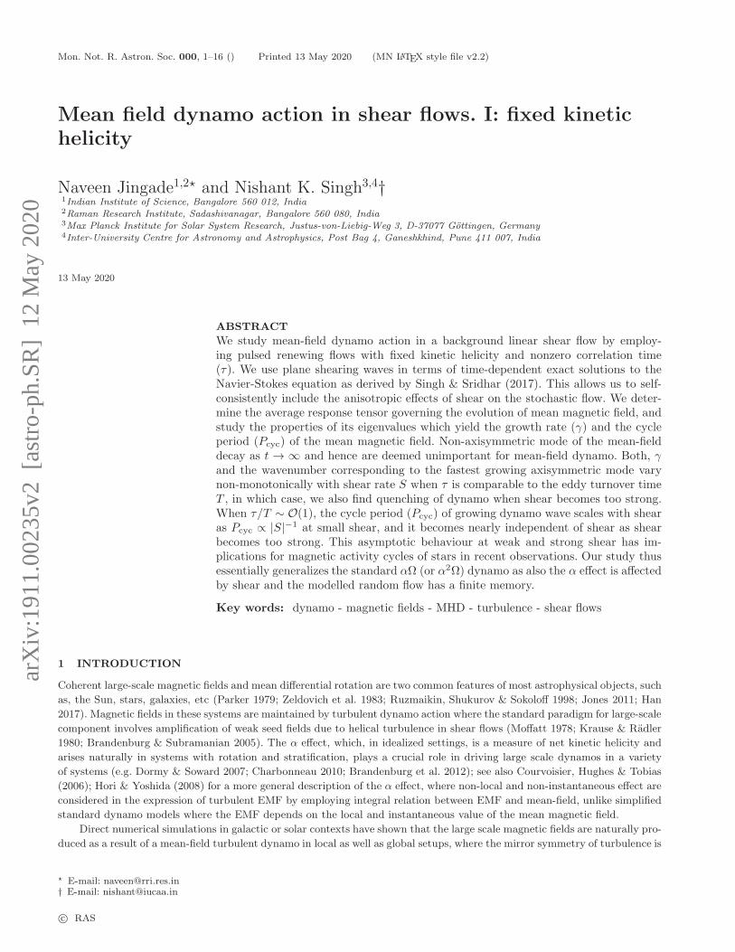
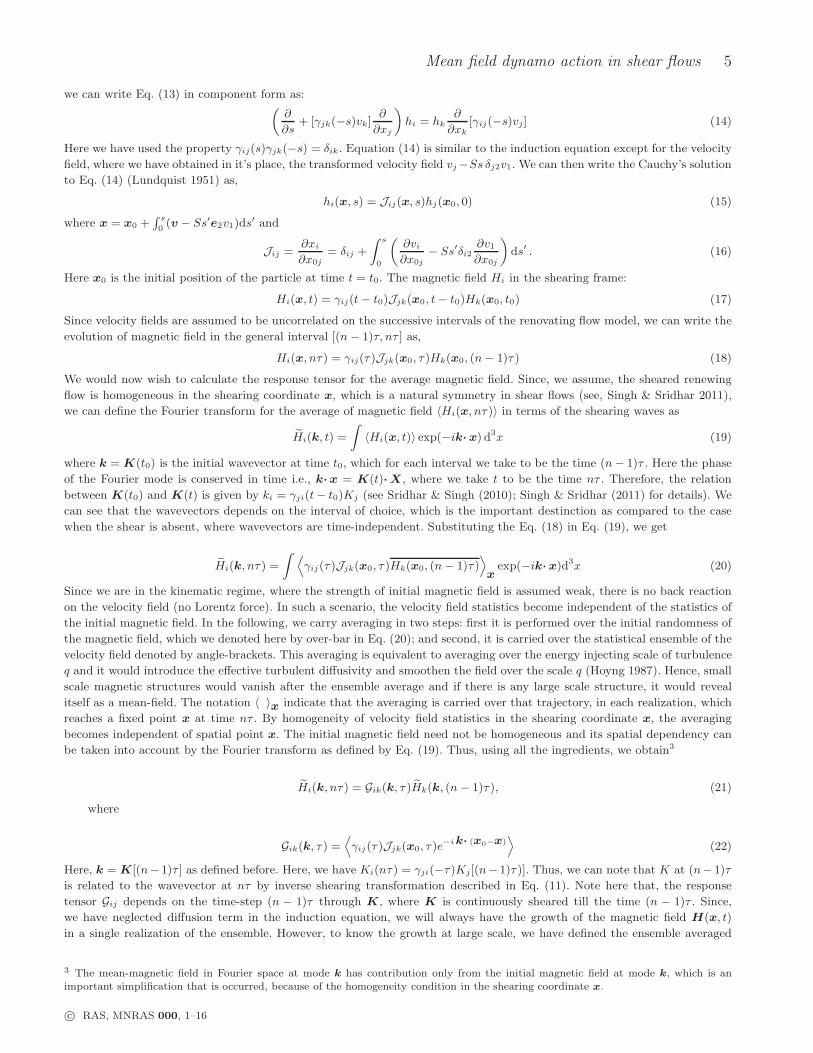
Figure 1. Contours of the magnitude of leading eigenvalue σ in k1 − k2 at k3 = 0.5, obtained at the end of first (left), third (middle)and fifth (right) interval n; time increases from left to right as n = t/τ .

determine the eigenvalues of the response tensor G which governs the evolution of mean magnetic field. The growth rate and

cycle period can then be obtained from Eq. 24. Below we discuss the non-axisymmetric and axisymmetric mean field dynamos.

We present our findings in the non-dimensional units, henceforth. All the quantities are suitably normalized with respect to

eddy turn-over time of the flow at the beginning of each interval, T = 1/qa, and the wave vector q. Quantities with over-tilde

are made dimensionless in this way, e.g., k = k/q, γ = γT , αij = αij/a, and so on.

3 DECAY OF NON-AXISYMMETRIC MODES OF MEAN MAGNETIC FIELD

We show in this subsection that the non-axisymmetric mode of the mean-magnetic field decays asymptotically. Since shearing

flows are anisotropic in all three directions, the eigenvalues of the response tensor for the magnetic field will also be anisotropic

in the directions of k1, k2 and k3. We have decomposed the magnetic field in the shearing waves (see Eq. (19)), where we

have used time dependent wave vector. If (k1, k2, k3) be the wave vector of the magnetic field at time t = 0, then at t = nτ ,

it would become (k1 − nSτ k2, k2, k3).

Let us denote the magnetic field by the column vector H and response tensor by the square matrix G (see Eq. (21)). Let

H0 be the initial magnetic field at t = 0, then the magnetic field at t = nτ is given by

Hn = Gn . . . G2G1H0 (29)

where Gn indicate the response tensor in nth interval with sheared wavevector (k1 − nSτ k2, k2, k3).

We now describe the procedure to determine Hn iteratively. At the end of the first interval, we get H1 = G1H0. We

find that one of the eigenvectors of G1 does not satisfy k·H0 = 0. Let V01 and V02 be the eigenvectors (with corresponding

eigenvalues being σ01 and σ02), such that, they are orthogonal to the direction of k. We can now express the initial magnetic

field in terms of the eigenvectors as

H0 = C01V01 + C02V02 (30)

where C01 and C02 are some complex constants. The quantity H1 thus becomes:

H1 = C01 σ01V01 + C02 σ02V02 (31)

For the next iteration, that is at t = 2τ , we have H2 = G2H1. The response tensor G2 is modified because the magnetic

field wave vector (k1, k2, k3) would shear to (k1 − Sτ k2, k2, k3). Hence, V01 and V02 will not anymore be the eigenvectors of

G2. We need to express the eigenvectors V01 and V02 in terms of the eigenvectors of G2. Similarly, let V11 and V12 be the

eigenvectors (with corresponding eigenvalues being σ11 and σ12) of the response tensor G2 orthogonal to the direction of

(k1 − Sτ k2, k2, k3). Then we have,

V01 = C(1)11 V11 + C

(1)12 V12 V02 = C

(2)11 V11 + C

(2)12 V12 (32)

where C(1)11 , C

(1)12 , C

(2)11 and C

(2)12 are again some complex constants.4 Using Eq. (32) in Eq. (31), we get

H2 = (. . . σ01σ11 + . . . σ02σ11)V11 + (. . . σ01σ12 + . . . σ02σ12)V12 (33)

4 Note here that, we have suppressed the third component of V01 and V02. Because at every interval we need to satisfy the solenoidalitycondition (∇·H=0).

c© RAS, MNRAS 000, 1–16

8 Jingade & Singh

20 40 60 80 100 120 140t/τ

0.6

0.7

0.8

0.9

1.0

1.1

1.2

1.3

1.4

|σ(k1−

Stk

2,k

2)|

S = − 1. 5τ = 1. 0k1 =0. 0

k2 =0. 0

k2 =0. 01

k2 =0. 02

20 40 60 80 100 120 140t/τ

10-4

10-3

10-2

10-1

100

101

102

103

104

105

|σ 01σ11σ21…

σn1|

k2 =0. 0

k2 =0. 01

k2 =0. 02

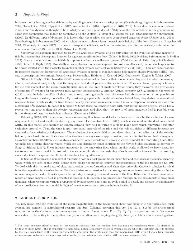
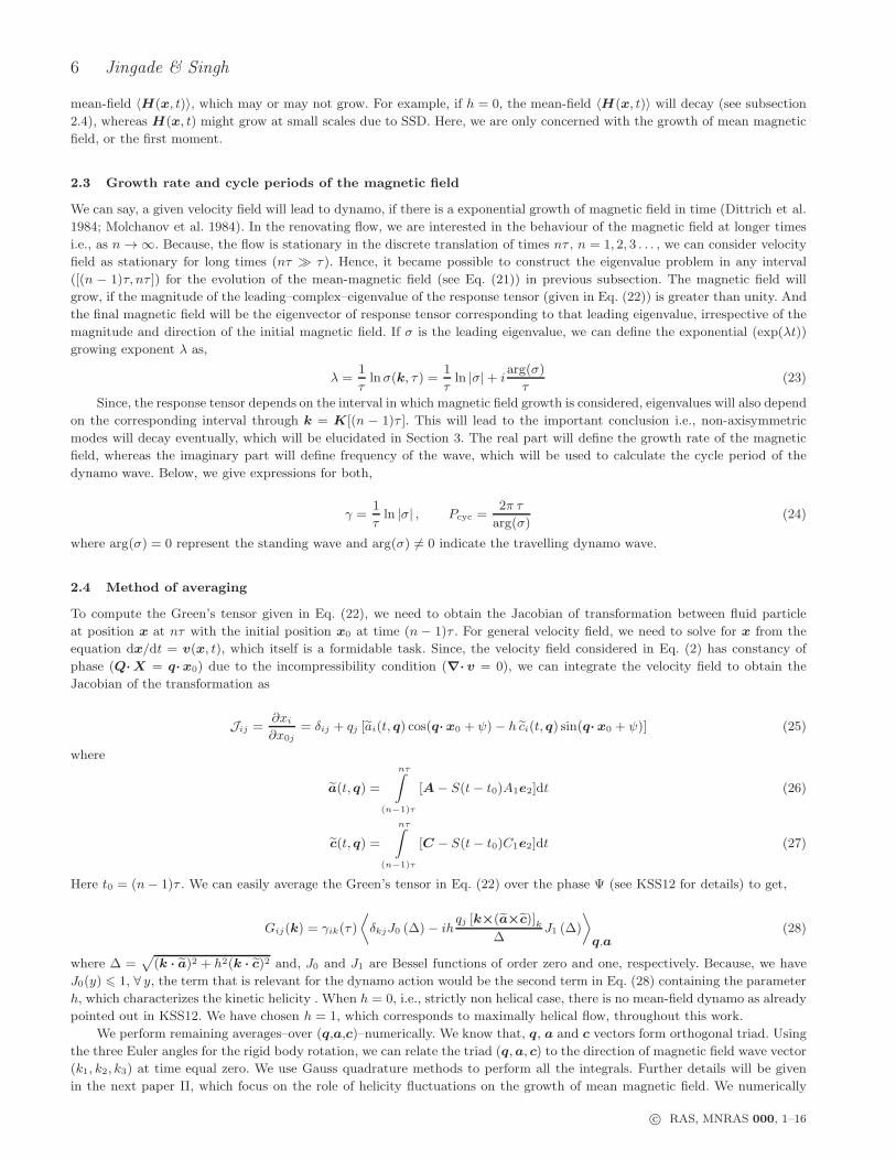
Figure 2. (Left) Magnitude of the leading eigenvalue and (right) cumulative product of the maximum eigenvalues as a function ofn = t/τ , i.e., the interval of the renovating flow.

where ellipsis indicate pre-multiplied factors, such as multiplication of complex coefficients. As we continue to iterate in the

above manner by expressing the preceding eigenvectors in terms of the current eigenvectors (like in Eq. (32)), we get 2n+1

terms for the magnetic field Hn at the end of nth interval; at every interval, the number of terms are doubled. Of the two

relevant eigenvectors at any interval, let us say that we have, |σn1| > |σn2|, then in those 2n+1 terms, there will be a term of the

kind σ01σ11σ21 . . . σn1 whose magnitude will be the largest compared to other terms. To demonstrate that non-axisymmetric

modes decay eventually, it is enough to show that this term decays after some interval of time.

In Figure 1 we have shown the magnitude of the largest eigenvalues σn1 in the k1 − k2 plane for k3 = 0.5 at the end

of first (t = τ ), third (t = 3τ ), and fifth (t = 5τ ) interval. We have highlighted the area where |σn1| > 1, which represents

the transient growth region. As time is increasing, the wave vector is continuously sheared in the k1 direction, the transient

growth region is stretched in the k1 direction, and it diminishes in the k2 direction. As time continues, the growth region aligns

with the k2 = 0 axis, and eventually vanishes. To make this point clear, let us consider the wavevectors, which lie close to

maxima of the contours shown in Figure 1, i.e., (0,0) in k1 − k2 plane. In the left panel of Figure 2, we have shown the largest

eigenvalue as the function of intervals for three different values of k2. When k2 = 0 (axisymmetric mode), the magnitude of the

largest eigenvalue remains constant as the wavevector (k1, 0, k3) remains same across the intervals. Therefore the cumulative

product of the magnitude of the eigenvalues |σ01σ11σ21 . . . σn1| = |σ01|n, increases monotonically leading to the exponential

growth of the axisymmetric mode of the magnetic field (see Figure 2: right panel, black solid line). For k2 6= 0, the wave

vectors are time dependent. As time increases, the value of k1 − St k2 increases (for negative S), eventually the wave vector

moves out of the transient growth region i.e., the region where |σn1| > 1 (see Figure 1). As shown in Figure 2 (left panel),

for k2 = 0.01 (k2 = 0.02), the magnitude of eigenvalue falls below unity around t = 80τ (t = 40τ ). The magnitude of the

cumulative product of the largest eigenvalues |σ01σ11σ21 . . . σn1| increases for some time (see right panel in Figure 2) and then

it starts to decrease, and falls below unity leading to the decay of the mode. Hence, non-axisymmetric modes will only have

transient growth before decaying eventually. Even though, the analysis of this section is made with the particular velocity

field, it’s validity remains general. Because, essential argument to show the asymptotic decay needs only two ingredients: the

magnetic wave vector is time-dependent, which is a consequence of background shear flow; and the growth region is limited

in the k-space, which is the consequence of the finite correlation of velocity field rather than it’s particular choice. Therefore,

in the kinematic dynamo regime, non-axisymmetric mode have no active role to play.

4 GROWTH OF AXISYMMETRIC MODES OF MEAN MAGNETIC FIELD

From now onward we focus only on the axisymmetric solutions for which k2 = 0, as the non-axisymmetric modes are expected

to decay as discussed above. Since, for axisymmetric modes the eigenvalues and eigenvectors are constant in time, we just

need to consider it’s growth rate in a single interval (see the black solid line in left panel of Figure 2). With σ being the leading

eigenvalue of the response tensor, we find that the magnetic field at the end of the nth interval is given by Hn = σnH0 where

H0 is the initial magnetic field, also assumed to be the corresponding eigenvector. Figure 3 shows contours of normalized

growth rate γ = γ T , with its positive values indicating exponentially growing solutions in k1-k3 plane for axisymmetric mean

field dynamos, as functions of the two parameters, the shear rate S, and the renovation time τ . Note that T = 1/qa is the

c© RAS, MNRAS 000, 1–16

Mean field dynamo action in shear flows 9

−1.5

−1.0

−0.5

0.0

0.5

1.0

1.5

k3

T |S|=0 τ/T=1 T |S|=0. 5 τ/T=1 T |S|=1. 5 τ/T=1 T |S|=2. 5 τ/T=1

−1.0−0.5 0.0 0.5 1.0 1.5

k1

−1.5

−1.0

−0.5

0.0

0.5

1.0

1.5

k3

T |S|=0 τ/T=2

−1.0−0.5 0.0 0.5 1.0 1.5

k1

T |S|=0. 5 τ/T=2

−1.0−0.5 0.0 0.5 1.0 1.5

k1

T |S|=1. 5 τ/T=2

−1.0−0.5 0.0 0.5 1.0 1.5

k1

T |S|=2. 5 τ/T=2

0.00

0.05

0.10

0.15

0.20

0.23

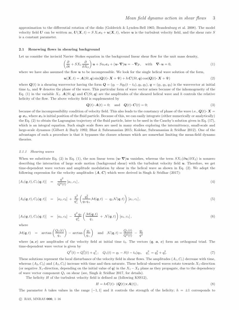
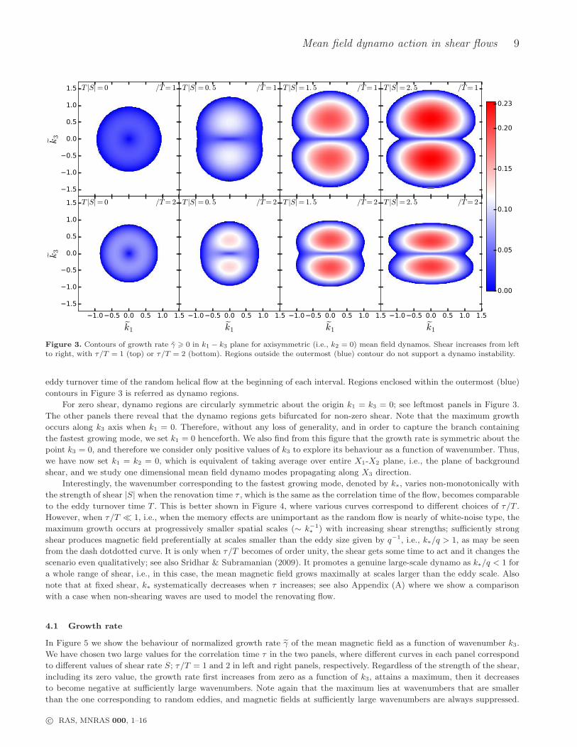
Figure 3. Contours of growth rate γ > 0 in k1 − k3 plane for axisymmetric (i.e., k2 = 0) mean field dynamos. Shear increases from leftto right, with τ/T = 1 (top) or τ/T = 2 (bottom). Regions outside the outermost (blue) contour do not support a dynamo instability.

eddy turnover time of the random helical flow at the beginning of each interval. Regions enclosed within the outermost (blue)

contours in Figure 3 is referred as dynamo regions.

For zero shear, dynamo regions are circularly symmetric about the origin k1 = k3 = 0; see leftmost panels in Figure 3.

The other panels there reveal that the dynamo regions gets bifurcated for non-zero shear. Note that the maximum growth

occurs along k3 axis when k1 = 0. Therefore, without any loss of generality, and in order to capture the branch containing

the fastest growing mode, we set k1 = 0 henceforth. We also find from this figure that the growth rate is symmetric about the

point k3 = 0, and therefore we consider only positive values of k3 to explore its behaviour as a function of wavenumber. Thus,

we have now set k1 = k2 = 0, which is equivalent of taking average over entire X1-X2 plane, i.e., the plane of background

shear, and we study one dimensional mean field dynamo modes propagating along X3 direction.

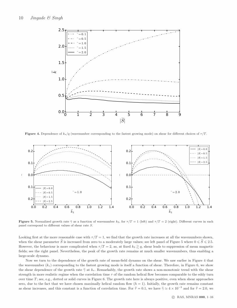
Interestingly, the wavenumber corresponding to the fastest growing mode, denoted by k∗, varies non-monotonically with

the strength of shear |S| when the renovation time τ , which is the same as the correlation time of the flow, becomes comparable

to the eddy turnover time T . This is better shown in Figure 4, where various curves correspond to different choices of τ/T .

However, when τ/T ≪ 1, i.e., when the memory effects are unimportant as the random flow is nearly of white-noise type, the

maximum growth occurs at progressively smaller spatial scales (∼ k−1∗ ) with increasing shear strengths; sufficiently strong

shear produces magnetic field preferentially at scales smaller than the eddy size given by q−1, i.e., k∗/q > 1, as may be seen

from the dash dotdotted curve. It is only when τ/T becomes of order unity, the shear gets some time to act and it changes the

scenario even qualitatively; see also Sridhar & Subramanian (2009). It promotes a genuine large-scale dynamo as k∗/q < 1 for

a whole range of shear, i.e., in this case, the mean magnetic field grows maximally at scales larger than the eddy scale. Also

note that at fixed shear, k∗ systematically decreases when τ increases; see also Appendix (A) where we show a comparison

with a case when non-shearing waves are used to model the renovating flow.

4.1 Growth rate

In Figure 5 we show the behaviour of normalized growth rate γ of the mean magnetic field as a function of wavenumber k3.

We have chosen two large values for the correlation time τ in the two panels, where different curves in each panel correspond

to different values of shear rate S; τ/T = 1 and 2 in left and right panels, respectively. Regardless of the strength of the shear,

including its zero value, the growth rate first increases from zero as a function of k3, attains a maximum, then it decreases

to become negative at sufficiently large wavenumbers. Note again that the maximum lies at wavenumbers that are smaller

than the one corresponding to random eddies, and magnetic fields at sufficiently large wavenumbers are always suppressed.

c© RAS, MNRAS 000, 1–16

10 Jingade & Singh

0 1 2 3 4 5 6 7 8 9

|S|0.0

0.5

1.0

1.5

2.0

2.5

k∗

τ=0. 1

τ=0. 5

τ=1. 0

τ=1. 5

τ=2. 0

Figure 4. Dependence of k∗/q (wavenumber corresponding to the fastest growing mode) on shear for different choices of τ/T .

0.0 0.2 0.4 0.6 0.8 1.0 1.2 1.4

k3

−0.2

−0.1

0.0

0.1

0.2

γ

τ=1. 0

|S|=0. 0

|S|=0. 5

|S|=1. 5

|S|=2. 5

0.0 0.2 0.4 0.6 0.8 1.0 1.2 1.4

k3

−0.2

−0.1

0.0

0.1

0.2

γ

τ=2. 0

|S|=0. 0

|S|=0. 5

|S|=1. 5

|S|=2. 5

Figure 5. Normalized growth rate γ as a function of wavenumber k3, for τ/T = 1 (left) and τ/T = 2 (right). Different curves in eachpanel correspond to different values of shear rate S.

Looking first at the more reasonable case with τ/T = 1, we find that the growth rate increases at all the wavenumbers shown,

when the shear parameter S is increased from zero to a moderately large values; see left panel of Figure 5 where 0 6 S 6 2.5.

However, the behaviour is more complicated when τ/T = 2, as, at fixed k3 & q, shear leads to suppression of mean magnetic

fields; see the right panel. Nevertheless, the peak of the growth rate remains at much smaller wavenumbers, thus enabling a

large-scale dynamo.

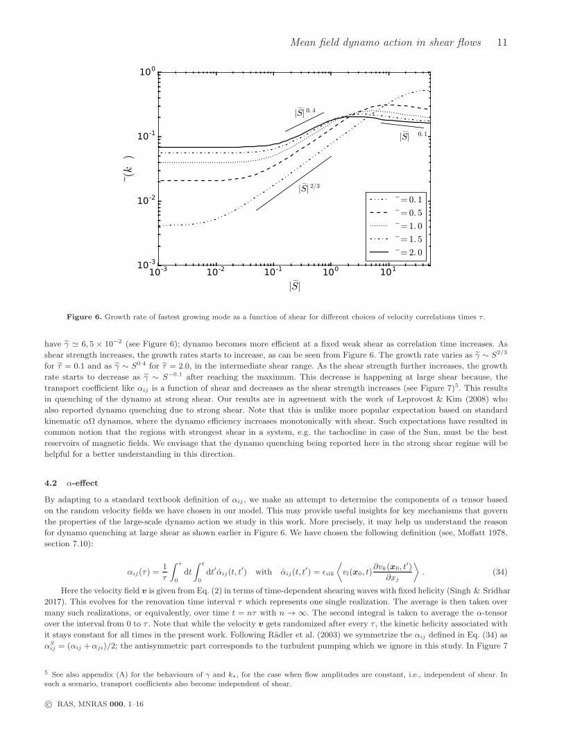
Now we turn to the dependence of the growth rate of mean-field dynamo on the shear. We saw earlier in Figure 4 that

the wavenumber (k∗) corresponding to the fastest growing mode is itself a function of shear. Therefore, in Figure 6, we show

the shear dependence of the growth rate γ at k∗. Remarkably, the growth rate shows a non-monotonic trend with the shear

strength in more realistic regime when the correlation time τ of the random helical flow becomes comparable to the eddy turn

over time T ; see, e.g., dotted or solid curves in Figure 6. The growth rate here is always positive, even when shear approaches

zero, due to the fact that we have chosen maximally helical random flow (h = 1). Initially, the growth rate remains constant

as shear increases, and this constant is a function of correlation time. For τ = 0.1, we have γ ≃ 4× 10−3 and for τ = 2.0, we

c© RAS, MNRAS 000, 1–16

Mean field dynamo action in shear flows 11

10-3 10-2 10-1 100 101

|S|10-3

10-2

10-1

100

γ(k

∗)

|S| 2/3

|S| − 0. 1

|S| 0. 4

τ=0. 1

τ=0. 5

τ=1. 0

τ=1. 5

τ=2. 0

Figure 6. Growth rate of fastest growing mode as a function of shear for different choices of velocity correlations times τ .

have γ ≃ 6, 5 × 10−2 (see Figure 6); dynamo becomes more efficient at a fixed weak shear as correlation time increases. As

shear strength increases, the growth rates starts to increase, as can be seen from Figure 6. The growth rate varies as γ ∼ S2/3

for τ = 0.1 and as γ ∼ S0.4 for τ = 2.0, in the intermediate shear range. As the shear strength further increases, the growth

rate starts to decrease as γ ∼ S−0.1 after reaching the maximum. This decrease is happening at large shear because, the

transport coefficient like αij is a function of shear and decreases as the shear strength increases (see Figure 7)5. This results

in quenching of the dynamo at strong shear. Our results are in agreement with the work of Leprovost & Kim (2008) who

also reported dynamo quenching due to strong shear. Note that this is unlike more popular expectation based on standard

kinematic αΩ dynamos, where the dynamo efficiency increases monotonically with shear. Such expectations have resulted in

common notion that the regions with strongest shear in a system, e.g. the tachocline in case of the Sun, must be the best

reservoirs of magnetic fields. We envisage that the dynamo quenching being reported here in the strong shear regime will be

helpful for a better understanding in this direction.

4.2 α-effect

By adapting to a standard textbook definition of αij , we make an attempt to determine the components of α tensor based

on the random velocity fields we have chosen in our model. This may provide useful insights for key mechanisms that govern

the properties of the large-scale dynamo action we study in this work. More precisely, it may help us understand the reason

for dynamo quenching at large shear as shown earlier in Figure 6. We have chosen the following definition (see, Moffatt 1978,

section 7.10):

αij(τ ) =1

τ

∫ τ

0

dt

∫ t

0

dt′αij(t, t′) with αij(t, t

′) = ǫilk

⟨vl(x0, t)

∂vk(x0, t′)

∂xj

⟩. (34)

Here the velocity field v is given from Eq. (2) in terms of time-dependent shearing waves with fixed helicity (Singh & Sridhar

2017). This evolves for the renovation time interval τ which represents one single realization. The average is then taken over

many such realizations, or equivalently, over time t = nτ with n → ∞. The second integral is taken to average the α-tensor

over the interval from 0 to τ . Note that while the velocity v gets randomized after every τ , the kinetic helicity associated with

it stays constant for all times in the present work. Following Radler et al. (2003) we symmetrize the αij defined in Eq. (34) as

αSij = (αij +αji)/2; the antisymmetric part corresponds to the turbulent pumping which we ignore in this study. In Figure 7

5 See also appendix (A) for the behaviours of γ and k∗, for the case when flow amplitudes are constant, i.e., independent of shear. Insuch a scenario, transport coefficients also become independent of shear.

c© RAS, MNRAS 000, 1–16

12 Jingade & Singh

0 2 4 6 8 10

|S|0.0

0.1

0.2

0.3

0.4

0.5

0.6

0.7

αS 11

τ=2. 0

τ=1. 0

τ=0. 5

0 2 4 6 8 10

|S|0.00

0.02

0.04

0.06

0.08

0.10

0.12

0.14

αS 12

τ=2. 0

τ=1. 0

τ=0. 5

0 2 4 6 8 10

|S|0.00

0.05

0.10

0.15

0.20

0.25

0.30

0.35

αS 22

τ=2. 0

τ=1. 0

τ=0. 5

0 2 4 6 8 10

|S|0.05

0.10

0.15

0.20

0.25

0.30

0.35

αS 33

τ=2. 0

τ=1. 0

τ=0. 5

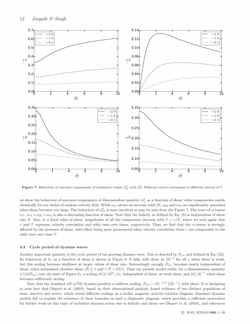
Figure 7. Behaviour of non-zero components of symmetric tensor αSij with |S|. Different curves correspond to different choices of τ .

we show the behaviour of non-zero components of dimensionless quantity αSij as a function of shear; other components vanish

identically for our choice of random velocity field. While α11 shows an increase with |S|, α22 and α33 are significantly quenched

when shear becomes too large. The behaviour of αS12 is more involved as may be seen from the Figure 7. The trace of α-tensor

i.e., α11 +α22 +α33 is also a decreasing function of shear. Note that the helicity as defined by Eq. (8) is independent of shear

rate S. Also, at a fixed value of shear, magnitudes of all the components increase with τ = τ/T , where we note again that

τ and T represent velocity correlation and eddy turn over times, respectively. Thus, we find that the α-tensor is strongly

affected by the presence of shear, with effect being more pronounced when velocity correlation times τ are comparable to the

eddy turn over time T .

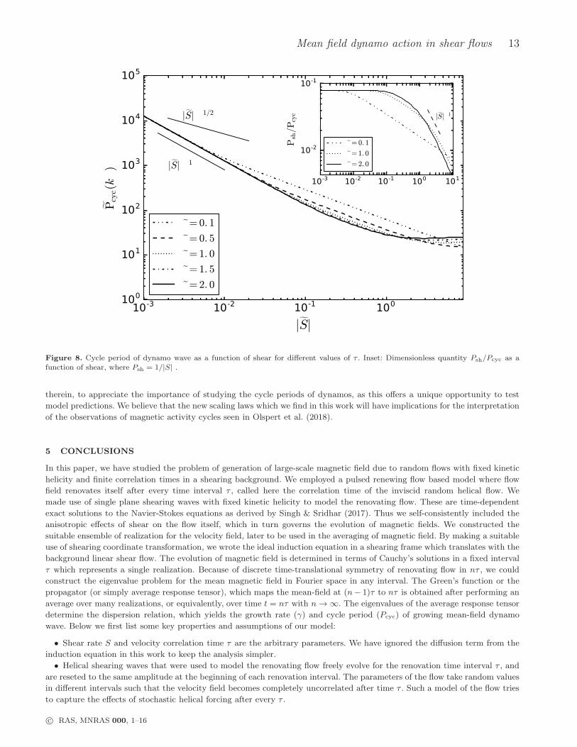
4.3 Cycle period of dynamo waves

Another important quantity is the cycle period of the growing dynamo wave. This is denoted by Pcyc and defined in Eq. (24).

Its behaviour at k∗ as a function of shear is shown in Figure 8. It falls with shear as |S|−1 for all τ when shear is weak,

but this scaling becomes shallower at larger values of shear rate. Interestingly enough, Pcyc becomes nearly independent of

shear, when normalized absolute shear |S| & 1 and τ/T ∼ O(1). Thus our present model yields, for a dimensionless quantity

1/(|S|Pcyc) (see the inset of Figure 8), a scaling of (i) |S|0, i.e., independent of shear, at weak shear, and (ii) |S|−1 when shear

becomes sufficiently strong.

Note that the standard αΩ (α2Ω) dynamo predicts a uniform scaling, Pcyc ∼ |S|−1/2 (|S|−1), with shear. It is intriguing

to note here that Olspert et al. (2018), based on their observational analysis, found evidence of two distinct population of

stars, inactive and active, which reveal different scalings in a stellar magnetic activity-rotation diagram. Standard dynamo

models fail to explain the existence of these branches in such a diagnostic diagram, which provides a sufficient motivation

for further work on this topic of turbulent dynamo action due to helicity and shear; see Olspert et al. (2018), and references

c© RAS, MNRAS 000, 1–16

Mean field dynamo action in shear flows 13

10-3 10-2 10-1 100

|S|100

101

102

103

104

105

Pcyc(k

∗)|S| − 1/2

|S| − 1

τ=0. 1

τ=0. 5

τ=1. 0

τ=1. 5

τ=2. 0

10-3 10-2 10-1 100 101

10-2

10-1

Psh/P

cyc |S|−1

τ=0. 1

τ=1. 0

τ=2. 0

Figure 8. Cycle period of dynamo wave as a function of shear for different values of τ . Inset: Dimensionless quantity Psh/Pcyc as afunction of shear, where Psh = 1/|S| .

therein, to appreciate the importance of studying the cycle periods of dynamos, as this offers a unique opportunity to test

model predictions. We believe that the new scaling laws which we find in this work will have implications for the interpretation

of the observations of magnetic activity cycles seen in Olspert et al. (2018).

5 CONCLUSIONS

In this paper, we have studied the problem of generation of large-scale magnetic field due to random flows with fixed kinetic

helicity and finite correlation times in a shearing background. We employed a pulsed renewing flow based model where flow

field renovates itself after every time interval τ , called here the correlation time of the inviscid random helical flow. We

made use of single plane shearing waves with fixed kinetic helicity to model the renovating flow. These are time-dependent

exact solutions to the Navier-Stokes equations as derived by Singh & Sridhar (2017). Thus we self-consistently included the

anisotropic effects of shear on the flow itself, which in turn governs the evolution of magnetic fields. We constructed the

suitable ensemble of realization for the velocity field, later to be used in the averaging of magnetic field. By making a suitable

use of shearing coordinate transformation, we wrote the ideal induction equation in a shearing frame which translates with the

background linear shear flow. The evolution of magnetic field is determined in terms of Cauchy’s solutions in a fixed interval

τ which represents a single realization. Because of discrete time-translational symmetry of renovating flow in nτ , we could

construct the eigenvalue problem for the mean magnetic field in Fourier space in any interval. The Green’s function or the

propagator (or simply average response tensor), which maps the mean-field at (n− 1)τ to nτ is obtained after performing an

average over many realizations, or equivalently, over time t = nτ with n→ ∞. The eigenvalues of the average response tensor

determine the dispersion relation, which yields the growth rate (γ) and cycle period (Pcyc) of growing mean-field dynamo

wave. Below we first list some key properties and assumptions of our model:

• Shear rate S and velocity correlation time τ are the arbitrary parameters. We have ignored the diffusion term from the

induction equation in this work to keep the analysis simpler.

• Helical shearing waves that were used to model the renovating flow freely evolve for the renovation time interval τ , and

are reseted to the same amplitude at the beginning of each renovation interval. The parameters of the flow take random values

in different intervals such that the velocity field becomes completely uncorrelated after time τ . Such a model of the flow tries

to capture the effects of stochastic helical forcing after every τ .

c© RAS, MNRAS 000, 1–16

14 Jingade & Singh

We studied the properties of growth rate and cycle periods of growing large-scale magnetic fields that are obtained by a

mean-field dynamo action due to helical stochastic flows in a background linear shear. We focused in the regime when memory

effects become important, i.e., when the response tensor or the turbulent EMF is affected by the time dependence of the mean

magnetic field. As clarified in Sridhar & Singh (2014), this is equivalent to the case when the random flows are correlated

for non-zero times, as in the white-noise case the generalized EMF with a history term through a time-integral reduces to a

simple expression leading to an instantaneous relation with the mean magnetic field. Our study thus essentially generalizes

the standard α2Ω dynamo model to now also include the memory effects, and tensorial nature of α while treating the shear

non-perturbatively.

(a) Non-axisymmetric (k2 6= 0) modes: We found that the non-axisymmetric modes eventually decay in time and therefore

are unimportant for late time structures of mean magnetic field. However, these modes decay in an interesting manner in that

the contours of the growth rate γ form an ellipse with properties resembling the one for resistive Green’s function which is

derived by Sridhar & Singh (2010) for nonzero η after ignoring the advection term. As we have ignored η in the present work,

the resemblance points to a notion of turbulent diffusivity ηt which typically augments η. The decay of such non-axisymmetric

modes may thus be used to determine ηt and this will be attempted in a future work.

(b) Axisymmetric (k2 = 0) modes: These are the only modes that survive and will determine the late time evolution of mean

magnetic field. Comparing our results of axisymmetric mean field dynamo with the predictions of standard αΩ dynamos, we

find that the behaviours of γ and Pcyc with shear strength |S| are even qualitatively different when τ/T ∼ O(1). Some notable

findings in the regime when memory effects become important, i.e. when τ/T ∼ O(1), are highlighted as follows:

(i) The growth rate γ and the wavenumber (k∗) corresponding to the fastest growing mode vary non-monotonically with

|S|; see Figures 4 and 6. We find the quenching of the dynamo when shear becomes sufficiently strong. This is in agreement

with the work of Leprovost & Kim (2008) who also reported dynamo quenching due to strong shear. Common notions that

the regions of strongest shear in an astrophysical object are the ideal reservoirs of magnetic fields may thus need to be revised.

In order to understand the cause of such a quenching of growth rate (γ), we made an attempt to determine the α tensor by

adapting to its simplified textbook definition. We found that the magnitude of the more relevant component α22 is significantly

suppressed at larger shear and this may have affected the growth of mean magnetic field.

(ii) At fixed S and τ , γ first increases from zero as a function of wavenumber, reaches a maximum, and turns negative at

much larger wavenumbers. The quantity k∗ is smaller than q, which is the eddy wavenumber determining the injection scale

(q−1) of kinetic energy, for a whole range of shear. Also, at fixed shear, k∗ systematically decreases when τ increases. This

promotes a genuine large-scale dynamo as magnetic fields grow maximally at scales (k−1∗ ) that are larger than eddy size (q−1).

(iii) Dynamo cycle period Pcyc exhibits different scaling relations with shear depending on the strength of the shear

parameter: Pcyc ∝ |S|−1 when shear is small, and it becomes independent of shear when shear becomes sufficiently strong.

This is very different from the predictions of standard αΩ dynamo model which leads to a uniform scaling, Pcyc ∝ |S|−1/2,

with shear.

Recent observational study by Olspert et al. (2018) on stellar magnetic activity cycles reveal two branches, active and

inactive, in a diagnostic activity-rotation diagram. More work is needed to fully understand the origin of these branches,

e.g., whether these trace two distinct population of stars or are somehow related to multiple cycles from the same star.

Nevertheless, such studies emphasize the need to focus on the dynamo cycle period Pcyc as this may have direct implications

for these observations. This motivated us to explore in detail the properties of Pcyc in our model. Interestingly enough, we

find two asymptotic branches when we look at the dimensionless quantity 1/|S|Pcyc ; see the inset of Figure 8. This quantity

is independent of shear when shear is weak, and varies as |S|−1 in the strong shear regime. It is useful to note that the

model predictions and scaling relations such as the ones reported here are often based on kinematic analysis, whereas the

observations relate to the nonlinear stage of stellar dynamos. Therefore it is important to investigate numerically how the

scalings of Pcyc are affected in the nonlinear stage. Nevertheless, we envisage that the new scaling laws being reported here

will be useful in the interpretations of observations of the magnetic activity cycles of stars.

ACKNOWLEDGMENTS

We thank the referee for useful comments and suggestions. We thank S. Sridhar for useful discussions and comments on the

manuscript. We thank Axel Brandenburg and Tarun Deep Saini for their support. NJ acknowledges the hospitality provided

by Nordita, Sweden, where this work began. NJ also thanks Chanda J. Jog for providing financial support.

c© RAS, MNRAS 000, 1–16

Mean field dynamo action in shear flows 15

REFERENCES

Bayly, B. J. & Childress, S., 1988, Geophys. Astrophys. Fluid Dynamics, 44, 211

Bhat, P. & Subramanian, K., 2015, Journal of Plasma Physics, 81, 5

Brandenburg, A., Bigazzi, A. & Subramanian, K., 2001, Mon. Not. R. Astr. Soc., 325, 685–692

Brandenburg, A., & Subramanian, K., 2005, Physics Reports, 417, 1–209.

Brandenburg, A., Radler, K.-H.,Rheinhardt, M. & Kapyla, P. J., 2008, ApJ, 676, 740–751.

Brandenburg, A., Sokoloff, D., & Subramanian, K., 2012, Spa. Sci. Rev., 169, 123–157.

Chamandy, L., & Singh, N. K., 2017, Mon. Not. R. Astr. Soc., 468, 3657

Charbonneau, P., 2010, Liv. Rev. Sol. Phys., 7, no 3.

Courvoisier, A., Hughes, D. A. & Tobias, S. M., 2006, Physical Review Letters, 96, 034503.

Dormy, E. & Soward, A. M., Mathematical Aspects of Natural Dynamos, CRC Press (2007)

Du, Y., & Ott, E., 1993, Journal of Fluid Mechanics, 257, 265-288

Finn, J. M., & Ott, E., 1988, Physics of Fluids, 31(10), 2992

Gilbert, A. D., & Bayly, B. J., 1992, Journal of Fluid Mechanics, 241, 199 (GB92).

Goldreich, P. & Lynden-Bell, D., 1965, Mon. Not. R. Astr. Soc., 130, 125.

Gressel, O., Elstner, D., Ziegler, U. & Rdiger, G., 2008, Astron. & Astrophys., 486, L35

Han, J. L., 2017, Ann. Rev. of Astron. and Astrophys., 55, 111–157.

Hori, K. & Yoshida, S., 2008, Geophys. Astrophys. Fluid Dynamics, 102, 601

Jones, C. A., 2011, Annual Review of Fluid Mechanics, 43, 583

Jingade, N. & Singh, Nishant K., 2020, Paper II in preparation

Kapyla, P. J., Mantere, M. J., & Brandenburg, A., 2012, Astrophys. J. Lett., 755, L22

Kapyla, M. J., Kapyla, P. J., Olspert, N., Brandenburg, A., Warnecke, J., Karak, B. B., & Pelt, J., 2016, Astron. & Astrophys.,

589, A56

Kapyla, M. J., Gent, F. A., Vaisala, M. S., & Sarson, G. R., 2018, Astron. & Astrophys., 611, A15

Kleeorin, N., & Rogachevskii, I., 2003, Physical Review E, 67, 026321.

Lundquist, S., 1951, Physical Review, 83, 307.

Kolekar, S., Subramanian, K., & Sridhar, S., 2012, Phys. Rev. E, 86, 026303 (KSS12).

Kraichnan, R. H., 1976, Journal of Fluid Mechanics, 75, 657.

Kraichnan, R. H., 1976, Journal of Fluid Mechanics, 77, 753.

Krause, F. & Radler, K.-H., Mean-field magnetohydrodynamics and dynamo theory; Pergamon Press, Oxford (1980).

Leprovost, N. & Kim, E., 2008, Physical Review Letters, 100, 144502.

Mitra, D., Kapyla, P. J., Tavakol, R., & Brandenburg, A., 2009, Astron. & Astrophys., 495, 1

Moffatt, H. K., Magnetic Field Generation in Electrically Conducting Fluids; Cambridge University Press, Cambridge (1978).

Molchanov, S. A. and Ruzmaikin, A. A. & Sokolov, D. D., 1984, Geophysical and Astrophysical Fluid Dynamics, 30, 241

Molchanov, S. A., Ruzmakin, A. A. & Sokolov, D. D., 1985, Sov. Phys. Usp. 28, 307.

Olspert, N., Lehtinen, J. J., Kapyla, M. J., Pelt, J., & Grigorievskiy, A., 2018, Astron. & Astrophys., 619, A6

Dittrich, P., Molchanov, S. A., Sokoloff, D. D. & Ruzmaikin, A. A., 1984, Astronomische Nachrichten, 305, 3, 119–125

Hoyng, P., 1987, Astron. & Astrophys., 171, 357–367

Parker, E. N., Cosmical magnetic fields: Their origin and their activity; Clarendon Press, Oxford; Oxford University Press,

New York (1979).

Radler, K.-H., Kleeorin, N., & Rogachevskii, I., 2003, Geophysical. and Astrophysical. Fluid Dynamics, 97, 249

Ruzmaikin, A. A., Shukurov, A. M. & Sokoloff, D. D., Magnetic Fields of Galaxies; Kluwer, Dodrecht (1998)

Schekochihin, A. A., Boldyrev, S. A. & Kulsrud, R. M., 2002, ApJ, 567, 828.

Singh, N. K. & Sridhar, S., 2011, Physical Review E, 83, 056309.

Singh, N. K. & Sridhar, S., 2017, Eur. Phys. J. Plus, 132, 403.

Sridhar, S. & Singh, N. K., 2010, Journal of Fluid Mechanics, 664, 265.

Sridhar, S. & Singh, N. K., 2014, Mon. Not. R. Astr. Soc., 445, 3770.

Sridhar, S. & Subramanian, K., 2009, Physical Review E, 80, 066315(1)–066315(13).

Sur, S., Brandenburg, A., & Subramanian, K., 2008, Mon. Not. R. Astr. Soc., 385, L15

Viviani, M., Kapyla, M. J., Warnecke, J., Kapyla, P. J. & Rheinhardt, M., 2019, eprint arXiv:1902.04019

Warnecke, J., Kapyla, P. J., Kapyla, M. J., & Brandenburg, A., 2014, Astrophys. J. Lett., 796, L12

Zeldovich, Ya. B., Ruzmaikin, A. A., & Sokoloff, D. D., Magnetic fields in astrophysics, Gordon & Breach, New York (1983)

Zeldovich, Ya. B., Ruzmaikin, A. A., Molchanov, S. A. & Sokoloff, D. D., 1984, J. Fluid Mech., 144, 1–11.

c© RAS, MNRAS 000, 1–16

16 Jingade & Singh

0 1 2 3 4 5 6 7 8 9

|S|0.2

0.4

0.6

0.8

1.0

1.2

k∗

Shearing wavesτ=2. 0

τ=1. 0

Non Shearing waves

0 1 2 3 4 5 6 7 8 9

|S|0.0

0.1

0.2

0.3

0.4

0.5

0.6

0.7

0.8

γ(k

∗)

Shearing wavesτ=2. 0

τ=1. 0

Non-Shearing waves

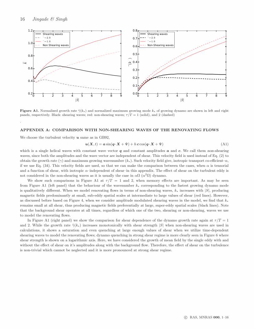
Figure A1. Normalized growth rate γ(k∗) and normalized maximum growing mode k∗ of growing dynamo are shown in left and rightpanels, respectively. Black: shearing waves; red: non-shearing waves; τ/T = 1 (solid), and 2 (dashed)

.

APPENDIX A: COMPARISON WITH NON-SHEARING WAVES OF THE RENOVATING FLOWS

We choose the turbulent velocity u same as in GB92,

u(X, t) = a sin(q·X +Ψ) + h c cos(q·X +Ψ) (A1)

which is a single helical waves with constant wave vector q and constant amplitudes a and c. We call them non-shearing

waves, since both the amplitudes and the wave vector are independent of shear. This velocity field is used instead of Eq. (2) to

obtain the growth rate (γ) and maximum growing wavenumber (k∗). Such velocity field give, isotropic transport co-efficient–α,

if we use Eq. (34). This velocity fields are used, so that we can make the comparison between the cases, when α is tensorial

and a function of shear, with isotropic α–independent of shear–in this appendix. The effect of shear on the turbulent eddy is

not considered in the non-shearing waves as it is usually the case in αΩ (α2Ω) dynamo.

We show such comparisons in Figure A1 at τ/T = 1 and 2, when memory effects are important. As may be seen

from Figure A1 (left panel) that the behaviour of the wavenumber k∗ corresponding to the fastest growing dynamo mode

is qualitatively different. When we model renovating flows in terms of non-shearing waves, k∗ increases with |S|, producing

magnetic fields predominantly at small, sub-eddy spatial scales at intermediate to large values of shear (red lines). However,

as discussed before based on Figure 4, when we consider amplitude modulated shearing waves in the model, we find that k∗remains small at all shear, thus producing magnetic fields preferentially at large, super-eddy spatial scales (black lines). Note

that the background shear operates at all times, regardless of which one of the two, shearing or non-shearing, waves we use

to model the renovating flows.

In Figure A1 (right panel) we show the comparison for shear dependence of the dynamo growth rate again at τ/T = 1

and 2. While the growth rate γ(k∗) increases monotonically with shear strength |S| when non-shearing waves are used in

calculations, it shows a saturation and even quenching at large enough values of shear when we utilize time-dependent

shearing waves to model the renovating flows; dynamo quenching in strong shear regime is more clearly seen in Figure 6 where

shear strength is shown on a logarithmic axis. Here, we have considered the growth of mean field by the single eddy with and

without the effect of shear on it’s amplitudes along with the background flow. Therefore, the effect of shear on the turbulence

is non-trivial which cannot be neglected and it is more pronounced at strong shear regime.

c© RAS, MNRAS 000, 1–16