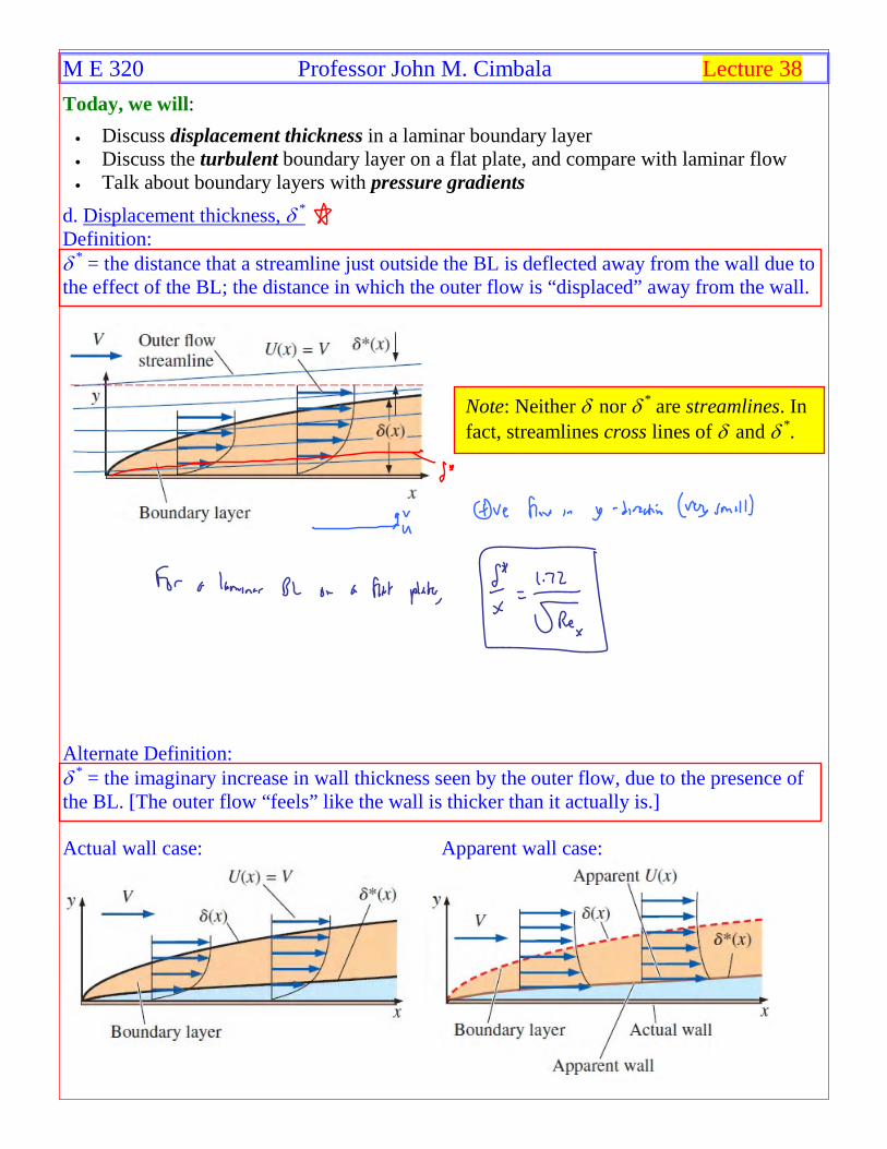
M E 320 Professor John M. Cimbala Lecture 38

Today, we will:

• Discuss displacement thickness in a laminar boundary layer • Discuss the turbulent boundary layer on a flat plate, and compare with laminar flow • Talk about boundary layers with pressure gradients

d. Displacement thickness, δ * Definition: δ * = the distance that a streamline just outside the BL is deflected away from the wall due to the effect of the BL; the distance in which the outer flow is “displaced” away from the wall.

Alternate Definition: δ * = the imaginary increase in wall thickness seen by the outer flow, due to the presence of the BL. [The outer flow “feels” like the wall is thicker than it actually is.] Actual wall case: Apparent wall case:

Note: Neither δ nor δ * are streamlines. In fact, streamlines cross lines of δ and δ *.

Practical example of the usefulness of displacement thickness: Wind tunnel design. In these exaggerated drawings, as the BL grows along the walls of the wind tunnel, the speed in the core flow U(x) must increase because the core flow “feels” like the wind tunnel walls are converging, due to the displacement thickness effect. Actual wall case: Apparent wall case:

To avoid this effect, and to keep U(x) constant, we would need to make the wind tunnel walls diverge out with downstream distance by the amount of the displacement thickness δ *: Actual wall case: Apparent wall case:

6. Turbulent Boundary Layer on a Flat Plate

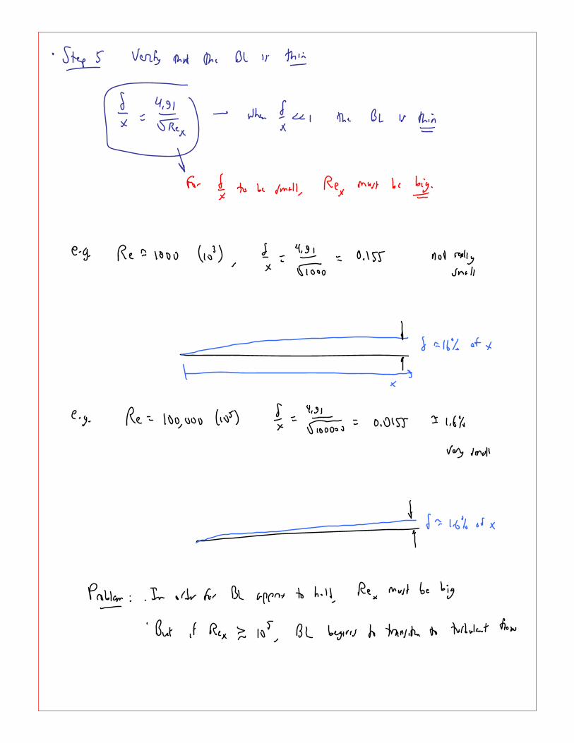
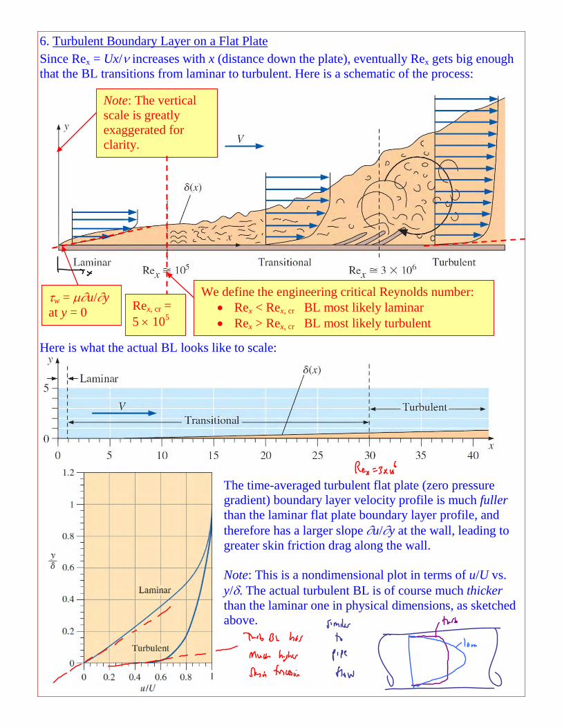
Since Rex = Ux/ν increases with x (distance down the plate), eventually Rex gets big enough that the BL transitions from laminar to turbulent. Here is a schematic of the process:

Here is what the actual BL looks like to scale:

The time-averaged turbulent flat plate (zero pressure gradient) boundary layer velocity profile is much fuller than the laminar flat plate boundary layer profile, and therefore has a larger slope ∂u/∂y at the wall, leading to greater skin friction drag along the wall. Note: This is a nondimensional plot in terms of u/U vs. y/δ. The actual turbulent BL is of course much thicker than the laminar one in physical dimensions, as sketched above.

We define the engineering critical Reynolds number: • Rex < Rex, cr BL most likely laminar • Rex > Rex, cr BL most likely turbulent

Note: The vertical scale is greatly exaggerated for clarity.

τw = μ∂u/∂y at y = 0 Rex, cr =

5 × 105

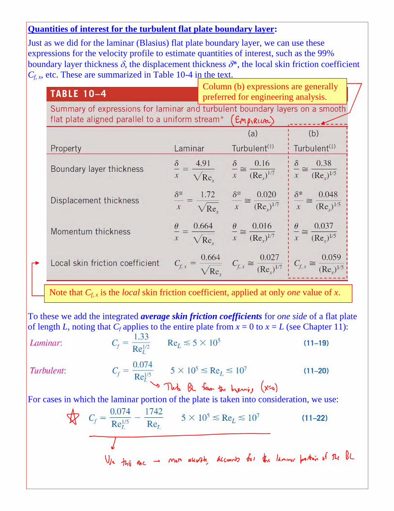
Quantities of interest for the turbulent flat plate boundary layer:

Just as we did for the laminar (Blasius) flat plate boundary layer, we can use these expressions for the velocity profile to estimate quantities of interest, such as the 99% boundary layer thickness δ, the displacement thickness δ*, the local skin friction coefficient Cf, x, etc. These are summarized in Table 10-4 in the text.

To these we add the integrated average skin friction coefficients for one side of a flat plate of length L, noting that Cf applies to the entire plate from x = 0 to x = L (see Chapter 11):

For cases in which the laminar portion of the plate is taken into consideration, we use:

Note that Cf, x is the local skin friction coefficient, applied at only one value of x.

Column (b) expressions are generally preferred for engineering analysis.

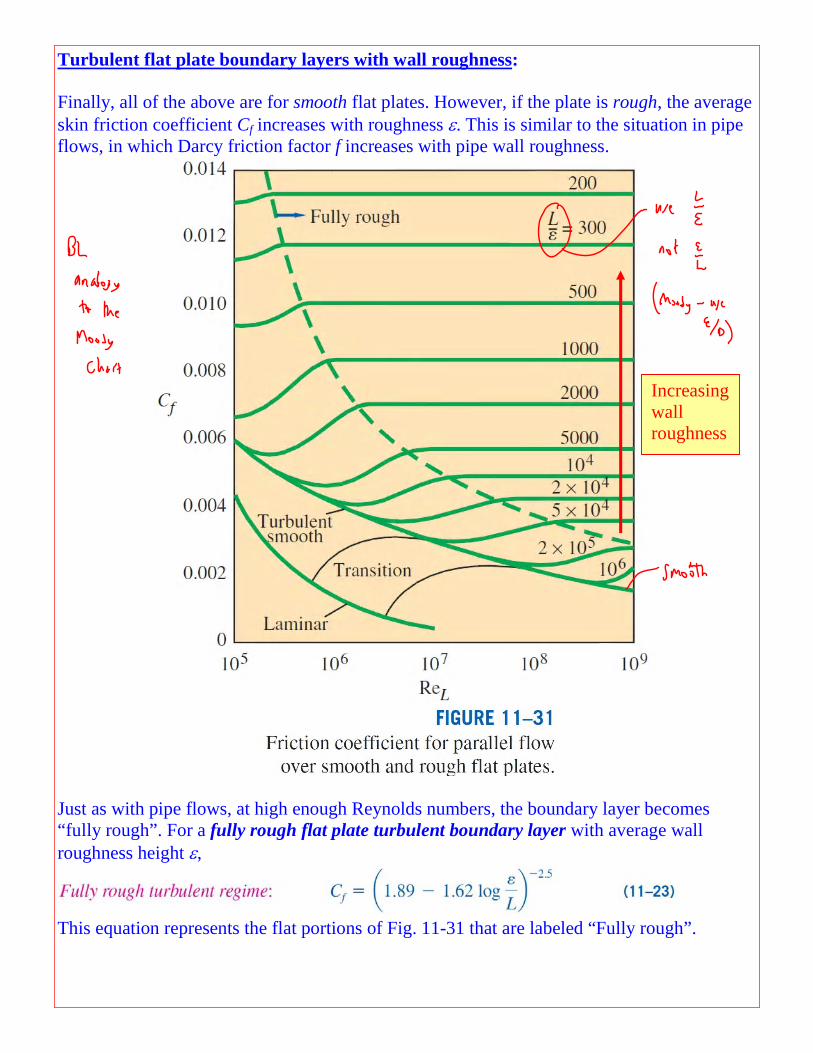
Turbulent flat plate boundary layers with wall roughness: Finally, all of the above are for smooth flat plates. However, if the plate is rough, the average skin friction coefficient Cf increases with roughness ε. This is similar to the situation in pipe flows, in which Darcy friction factor f increases with pipe wall roughness.

Just as with pipe flows, at high enough Reynolds numbers, the boundary layer becomes “fully rough”. For a fully rough flat plate turbulent boundary layer with average wall roughness height ε,

This equation represents the flat portions of Fig. 11-31 that are labeled “Fully rough”.

Increasing wall roughness

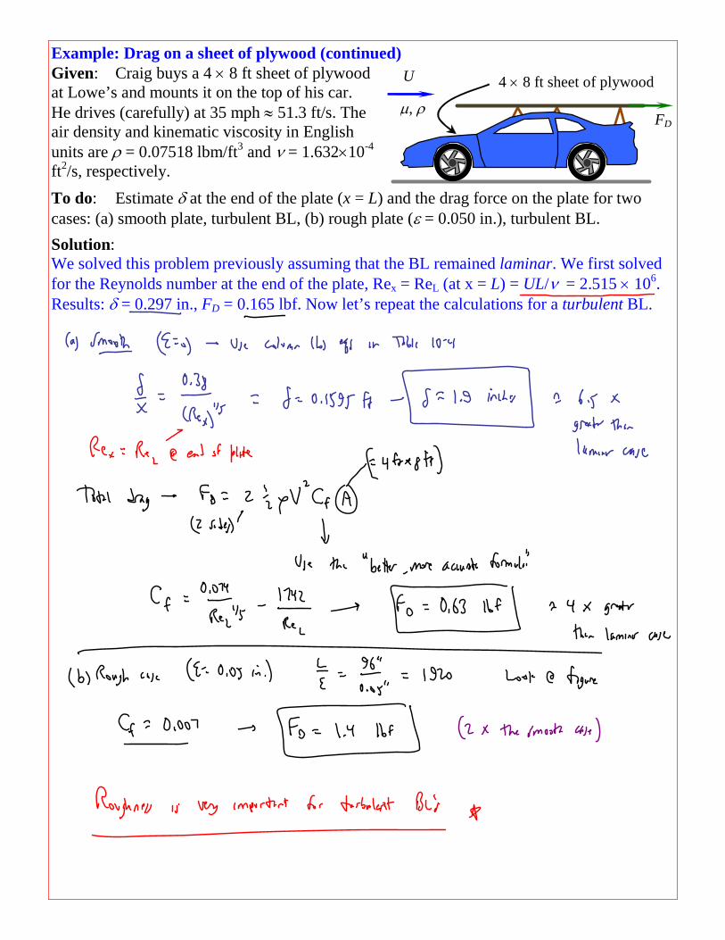
Example: Drag on a sheet of plywood (continued) Given: Craig buys a 4 × 8 ft sheet of plywood at Lowe’s and mounts it on the top of his car. He drives (carefully) at 35 mph ≈ 51.3 ft/s. The air density and kinematic viscosity in English units are ρ = 0.07518 lbm/ft3 and ν = 1.632×10-4 ft2/s, respectively.

To do: Estimate δ at the end of the plate (x = L) and the drag force on the plate for two cases: (a) smooth plate, turbulent BL, (b) rough plate (ε = 0.050 in.), turbulent BL.

Solution: We solved this problem previously assuming that the BL remained laminar. We first solved for the Reynolds number at the end of the plate, Rex = ReL (at x = L) = UL/ν = 2.515 × 106. Results: δ = 0.297 in., FD = 0.165 lbf. Now let’s repeat the calculations for a turbulent BL.

U

μ, ρ

4 × 8 ft sheet of plywood

FD

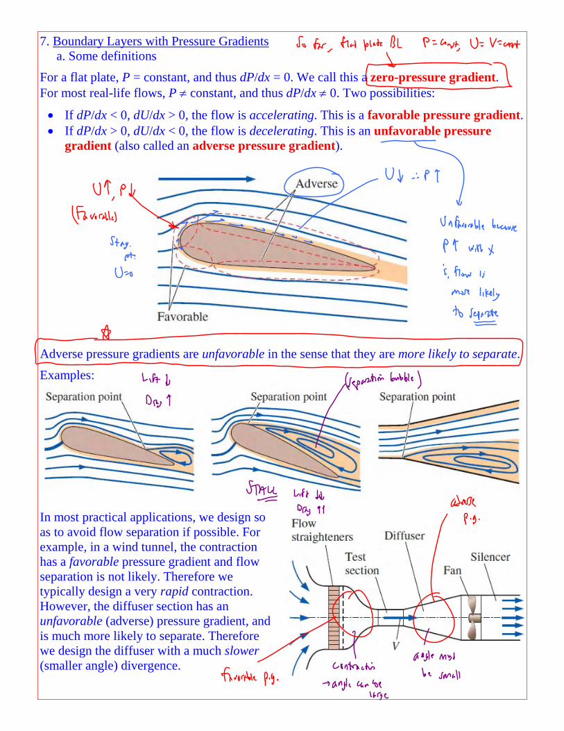
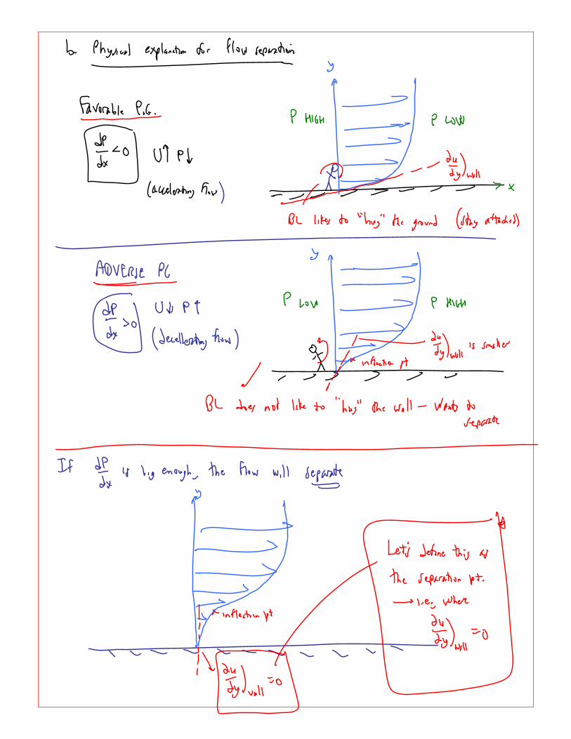
7. Boundary Layers with Pressure Gradients a. Some definitions

For a flat plate, P = constant, and thus dP/dx = 0. We call this a zero-pressure gradient. For most real-life flows, P ≠ constant, and thus dP/dx ≠ 0. Two possibilities:

• If dP/dx < 0, dU/dx > 0, the flow is accelerating. This is a favorable pressure gradient. • If dP/dx > 0, dU/dx < 0, the flow is decelerating. This is an unfavorable pressure

gradient (also called an adverse pressure gradient).

Adverse pressure gradients are unfavorable in the sense that they are more likely to separate.

Examples:

In most practical applications, we design so as to avoid flow separation if possible. For example, in a wind tunnel, the contraction has a favorable pressure gradient and flow separation is not likely. Therefore we typically design a very rapid contraction. However, the diffuser section has an unfavorable (adverse) pressure gradient, and is much more likely to separate. Therefore we design the diffuser with a much slower (smaller angle) divergence.