Maxwell’s Equations for Magnets -...
54
THE CERN ACCELERATOR SCHOOL Maxwell’s Equations for Magnets Part II: Realistic Fields Andy Wolski The Cockcroft Institute, and the University of Liverpool, UK CAS Specialised Course on Magnets Bruges, Belgium, June 2009
Transcript of Maxwell’s Equations for Magnets -...
THE CERN ACCELERATOR SCHOOL
Maxwell’s Equations for Magnets
Part II: Realistic Fields
Andy Wolski
The Cockcroft Institute, and the University of Liverpool, UK
CAS Specialised Course on MagnetsBruges, Belgium, June 2009
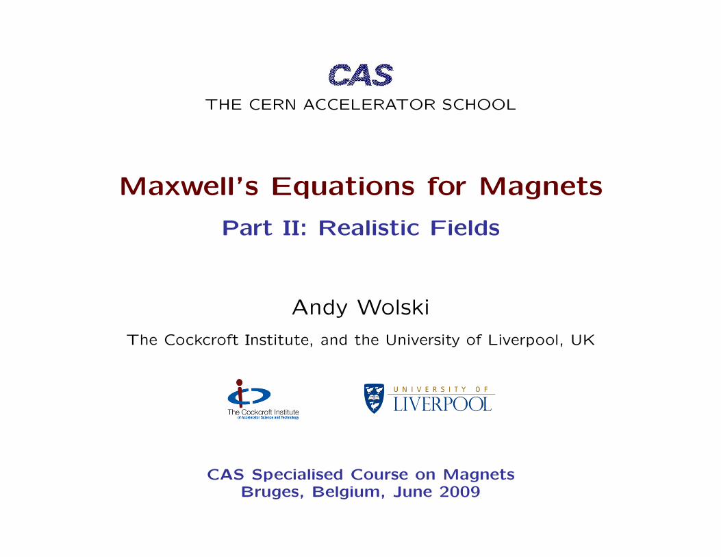
Key results from Lecture 1
In the first lecture, we saw that multipole fields of the form:
By + iBx = Cn(x+ iy)n−1 = Cnrn−1ei(n−1)θ (1)
with Bz = constant, provided valid solutions to Maxwell’s
equations in free space.
We also saw that such a field could be generated by a current
flowing parallel to the z-axis, on a cylinder of radius r0, with
distribution:
I(θ) = In cosn(θ − θn). (2)
In this case, the field is given by:
By + iBx =µ0In
2r0e−inθn
(r
r0
)n−1
ei(n−1)θ. (3)
Maxwell’s Equations 1 Part 2: Realistic Fields

Key results from Lecture 1
Multipole fields can also be generated by currents flowing inwires wound around iron poles. For a pure 2n-pole field, theshape of the surface of the iron pole must match a surface ofconstant scalar potential, Φ, given by:
Φ = −|Cn|rn
nsinn(θ − θn). (4)
The field is given by:
~B = −∇Φ. (5)
If each pole in an “ideal” 2n-pole magnet is wound with N
turns of wire carrying current I, then the multipole gradient ofthe field is:
∂n−1By
∂xn−1=n!µ0NI
rn0, (6)
where r0 is the radius of the largest cylinder that can beinscribed between the poles.
Maxwell’s Equations 2 Part 2: Realistic Fields

Goals for Lecture 2
In this lecture, we shall go beyond the idealised geometries and
materials that we assumed in Lecture 1, to consider more
realistic magnets. In particular, we shall:
1. deduce that the symmetry of a magnet imposes constraints
on the possible multipole field components, even if we relax
the constraints on the material properties and other
geometrical properties;
2. consider different techniques for deriving the multipole field
components from measurements of the fields within a
magnet;
3. discuss the solutions to Maxwell’s equations that may be
used for describing fields in three dimensions.
Maxwell’s Equations 3 Part 2: Realistic Fields

Allowed and forbidden harmonics
In general, from equation (1), a pure 2n-pole field can be
written:
By + iBx = |Cn|e−inθnrn−1ei(n−1)θ, (7)
where r and θ are the polar coordinates within the magnet, and
θn is the angle by which the magnet is rolled around the z axis.
We cannot design a realistic magnet to produce a pure 2n-pole
field. The materials will have finite permeability and finite
dimensions, and may saturate.
More generally, a field consists of a superposition of 2n-pole
fields:
By + iBx =∞∑n=1
|Cn|e−inθnrn−1ei(n−1)θ. (8)
Maxwell’s Equations 4 Part 2: Realistic Fields
Allowed and forbidden harmonics
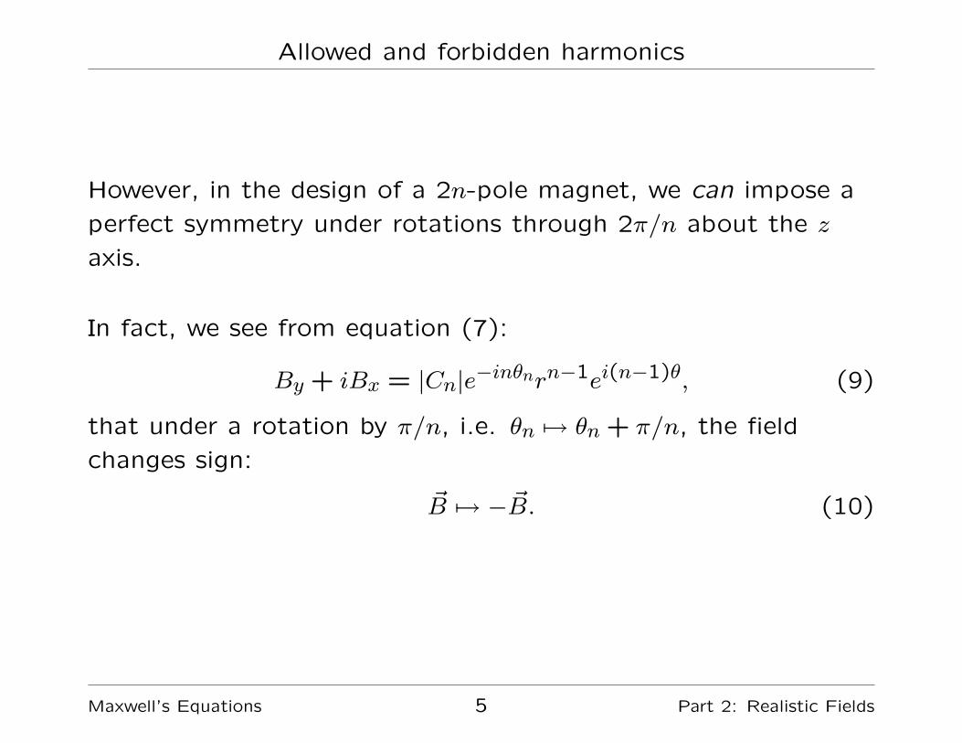
However, in the design of a 2n-pole magnet, we can impose a
perfect symmetry under rotations through 2π/n about the z
axis.
In fact, we see from equation (7):
By + iBx = |Cn|e−inθnrn−1ei(n−1)θ, (9)
that under a rotation by π/n, i.e. θn 7→ θn + π/n, the field
changes sign:
~B 7→ − ~B. (10)
Maxwell’s Equations 5 Part 2: Realistic Fields
Allowed and forbidden harmonics
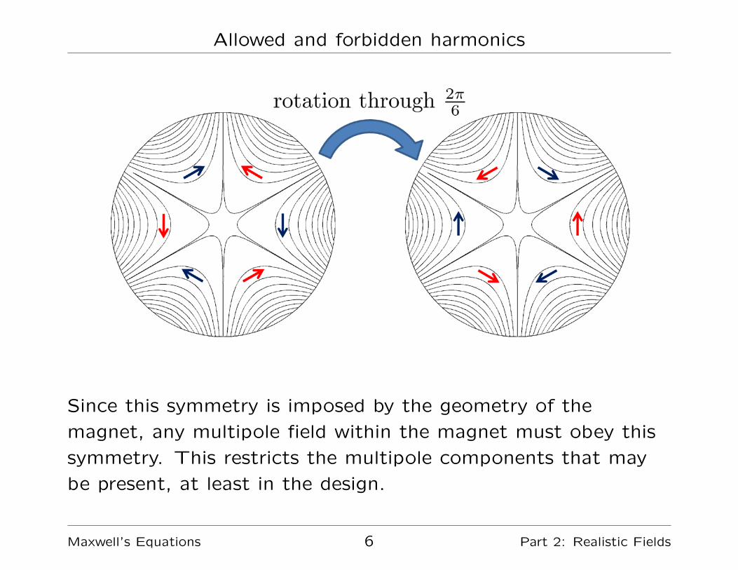
Since this symmetry is imposed by the geometry of the
magnet, any multipole field within the magnet must obey this
symmetry. This restricts the multipole components that may
be present, at least in the design.
Maxwell’s Equations 6 Part 2: Realistic Fields
Allowed and forbidden harmonics
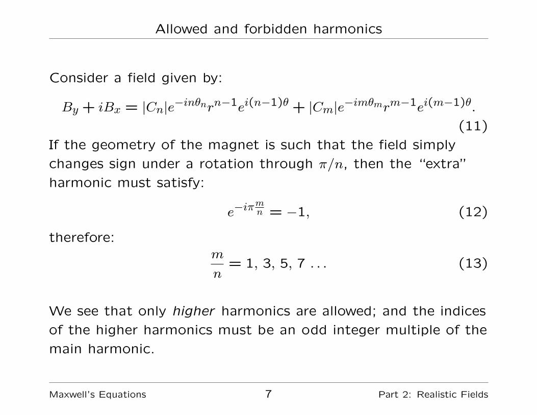
Consider a field given by:
By + iBx = |Cn|e−inθnrn−1ei(n−1)θ + |Cm|e−imθmrm−1ei(m−1)θ.
(11)
If the geometry of the magnet is such that the field simply
changes sign under a rotation through π/n, then the “extra”
harmonic must satisfy:
e−iπmn = −1, (12)
therefore:m
n= 1, 3, 5, 7 . . . (13)
We see that only higher harmonics are allowed; and the indices
of the higher harmonics must be an odd integer multiple of the
main harmonic.
Maxwell’s Equations 7 Part 2: Realistic Fields
Allowed and forbidden harmonics
Maxwell’s Equations 8 Part 2: Realistic Fields
Allowed and forbidden harmonics
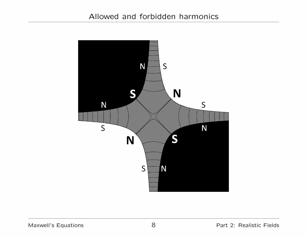
For a dipole, n = 1, so the allowed harmonics are m = 3,5,7 . . .
For a quadrupole, n = 2, and the allowed harmonics are
m = 6,10,14 . . .
Of course, this argument cannot tell us the strengths of the
allowed harmonics: those depend on the details of the design.
It is also a fact that a magnet, when fabricated, will never
exhibit perfectly the symmetry with which it was designed.
Therefore, a real physical magnet will generally include all
harmonics to some extent, not just the harmonics allowed by
the ideal symmetry.
However, for a carefully fabricated magnet, the harmonics
forbidden by the ideal symmetry should be small in comparison
to the allowed harmonics; and it should be possible to predict
the sizes of the allowed harmonics accurately from the design.
Maxwell’s Equations 9 Part 2: Realistic Fields
Measuring multipoles
Knowing the multipole components of magnets in an
accelerator is important for understanding the beam dynamics.
Construction tolerances will mean that the strengths of the
multipoles present in the magnet will differ from those in the
design.
This leads us to consider how to determine the multipole
components from measurements of the magnetic field.
There are many possible approaches to the problem: we shall
consider two, for illustration, and only go as far as necessary to
understand some of the pros and cons.
Maxwell’s Equations 10 Part 2: Realistic Fields
Measuring multipoles 1: Cartesian basis
The field may be represented as:
By + iBx =∑nCn(x+ iy)n−1, (14)
where the real parts of the coefficients Cn give the normal
multipole strengths, and the imaginary parts give the skew
multipole strengths.
If we take a set of measurements of By and Bx along the x
axis, then y = 0 at each measurement point, and the normal
multipoles can be found by fitting a polynomial to By vs x, and
the skew multipoles can be found by fitting a polynomial to Bx
vs x.
Let us see how this works with some invented data...
Maxwell’s Equations 11 Part 2: Realistic Fields
Measuring multipoles 1: Cartesian basis
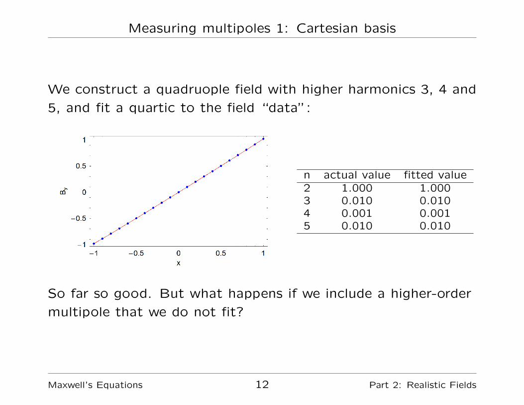
We construct a quadruople field with higher harmonics 3, 4 and
5, and fit a quartic to the field “data”:
n actual value fitted value2 1.000 1.0003 0.010 0.0104 0.001 0.0015 0.010 0.010
So far so good. But what happens if we include a higher-order
multipole that we do not fit?
Maxwell’s Equations 12 Part 2: Realistic Fields
Measuring multipoles 1: Cartesian basis
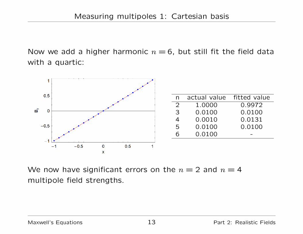
Now we add a higher harmonic n = 6, but still fit the field data
with a quartic:
n actual value fitted value2 1.0000 0.99723 0.0100 0.01004 0.0010 0.01315 0.0100 0.01006 0.0100 -
We now have significant errors on the n = 2 and n = 4
multipole field strengths.
Maxwell’s Equations 13 Part 2: Realistic Fields
Measuring multipoles 1: Cartesian basis
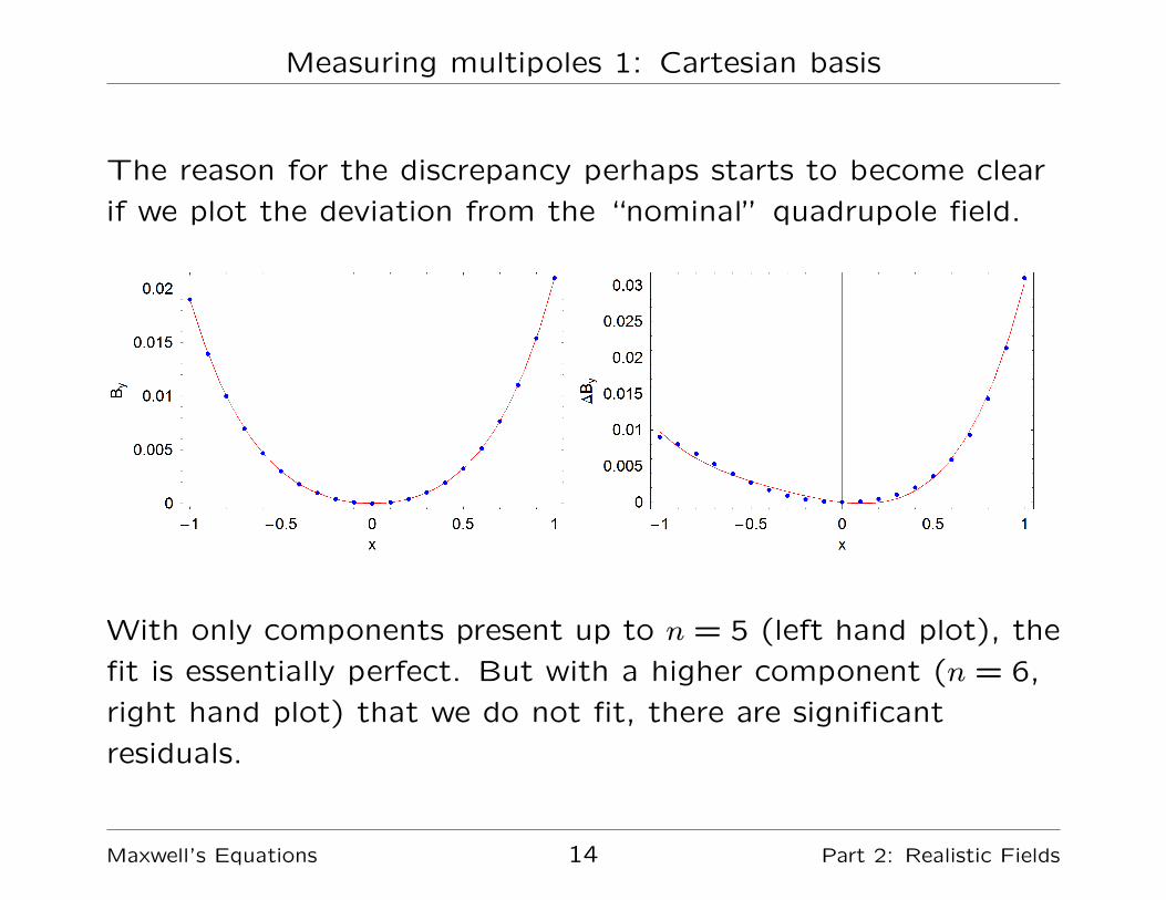
The reason for the discrepancy perhaps starts to become clear
if we plot the deviation from the “nominal” quadrupole field.
With only components present up to n = 5 (left hand plot), the
fit is essentially perfect. But with a higher component (n = 6,
right hand plot) that we do not fit, there are significant
residuals.
Maxwell’s Equations 14 Part 2: Realistic Fields
Measuring multipoles 1: Cartesian basis
The real problem is that mathematically, the basis functions
that we use to fit the data (monomials in x and, possibly, y)
are not orthogonal. This means that data constructed from
one monomial can be fitted, with non-zero strength, with a
completely different monomial.
Although this does not invalidate the technique altogether, it
does make it a little difficult to apply accurately. Ideally, we
need to know in advance which multipole components are
present.
However, there is a more robust technique...
Maxwell’s Equations 15 Part 2: Realistic Fields
Measuring multipoles 2: Polar basis
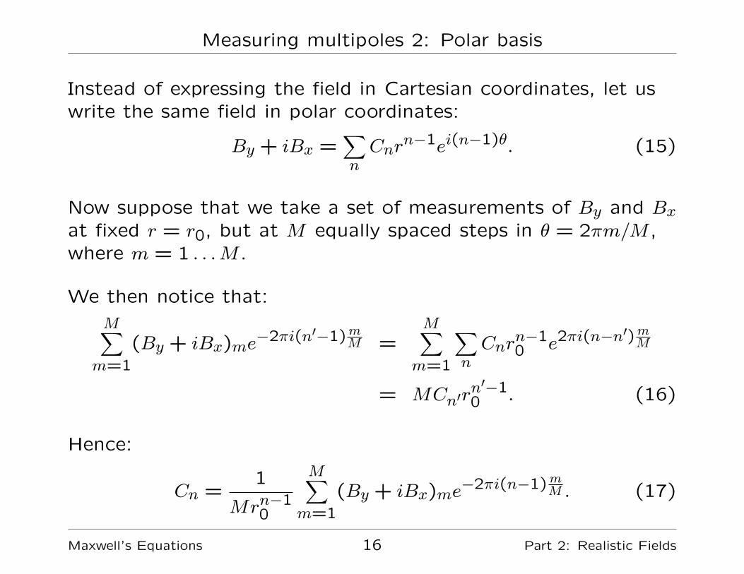
Instead of expressing the field in Cartesian coordinates, let uswrite the same field in polar coordinates:
By + iBx =∑nCnr
n−1ei(n−1)θ. (15)
Now suppose that we take a set of measurements of By and Bxat fixed r = r0, but at M equally spaced steps in θ = 2πm/M ,where m = 1 . . .M .
We then notice that:
M∑m=1
(By + iBx)me−2πi(n′−1)mM =
M∑m=1
∑nCnr
n−10 e2πi(n−n
′)mM
= MCn′rn′−10 . (16)
Hence:
Cn =1
Mrn−10
M∑m=1
(By + iBx)me−2πi(n−1)mM . (17)
Maxwell’s Equations 16 Part 2: Realistic Fields

Measuring multipoles 2: Polar basis
The advantage of using polar coordinates, over Cartesian
coordinates, is that the basis functions, ei(n−1)θ, are
orthogonal. Mathematically, we have:
M∑m=1
e2πi(n−1)mM e−2πi(n′−1)mM =
0 if n 6= n′
M if n = n′(18)
The orthogonality means that the value we determine for one
multipole component is completely unaffected by the presence
of other multipole components.
Determining the multipole coefficients Cn amounts to carrying
out a discrete Fourier transform on the field data measured on
a cylinder inscribed through the magnet.
Maxwell’s Equations 17 Part 2: Realistic Fields
Measuring multipoles 2: Polar basis
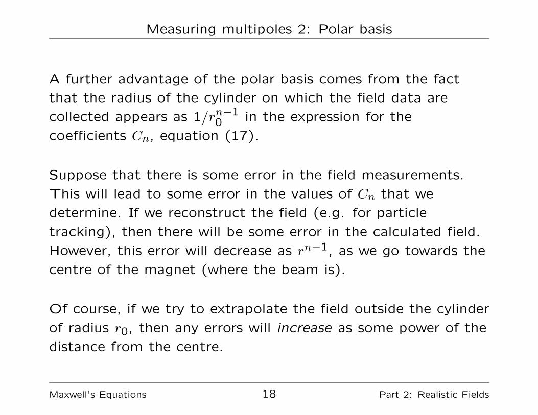
A further advantage of the polar basis comes from the fact
that the radius of the cylinder on which the field data are
collected appears as 1/rn−10 in the expression for the
coefficients Cn, equation (17).
Suppose that there is some error in the field measurements.
This will lead to some error in the values of Cn that we
determine. If we reconstruct the field (e.g. for particle
tracking), then there will be some error in the calculated field.
However, this error will decrease as rn−1, as we go towards the
centre of the magnet (where the beam is).
Of course, if we try to extrapolate the field outside the cylinder
of radius r0, then any errors will increase as some power of the
distance from the centre.
Maxwell’s Equations 18 Part 2: Realistic Fields
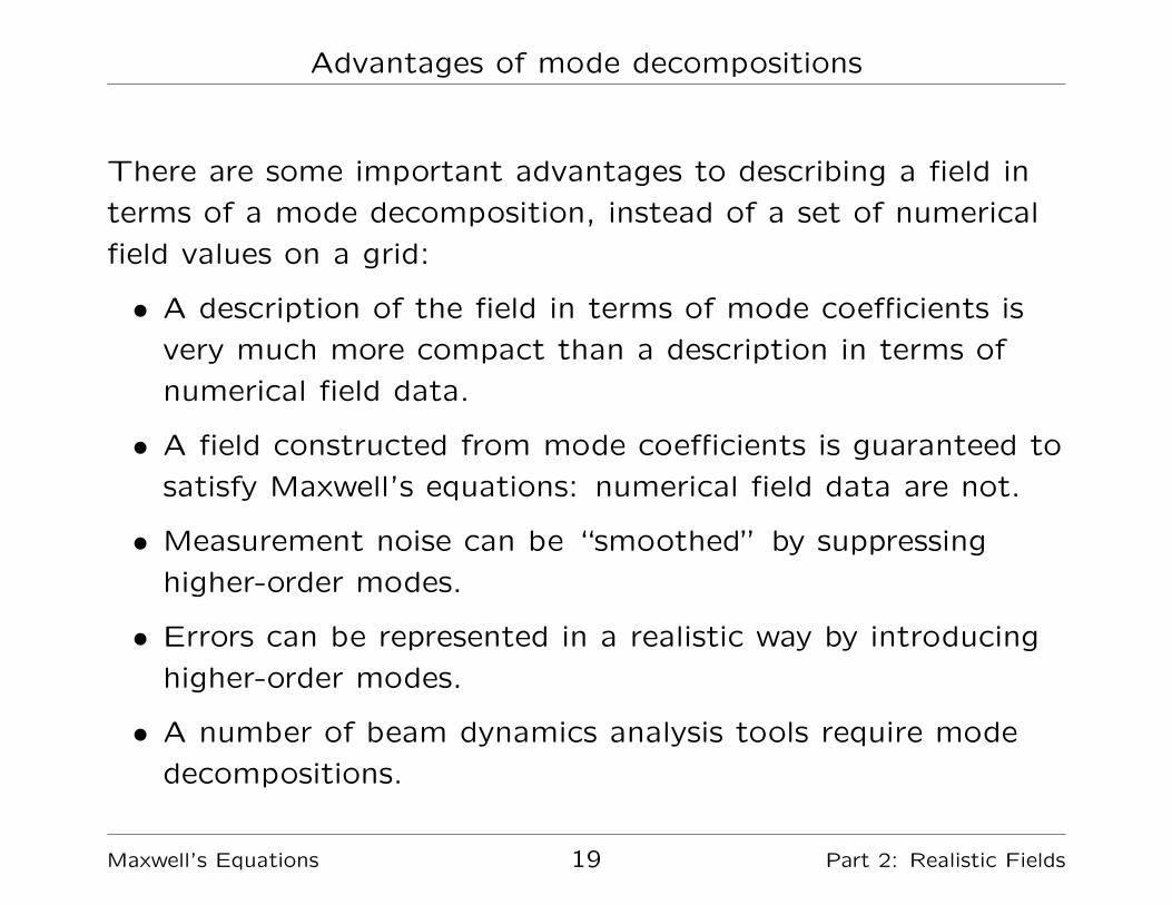
Advantages of mode decompositions
There are some important advantages to describing a field in
terms of a mode decomposition, instead of a set of numerical
field values on a grid:
• A description of the field in terms of mode coefficients is
very much more compact than a description in terms of
numerical field data.
• A field constructed from mode coefficients is guaranteed to
satisfy Maxwell’s equations: numerical field data are not.
• Measurement noise can be “smoothed” by suppressing
higher-order modes.
• Errors can be represented in a realistic way by introducing
higher-order modes.
• A number of beam dynamics analysis tools require mode
decompositions.
Maxwell’s Equations 19 Part 2: Realistic Fields
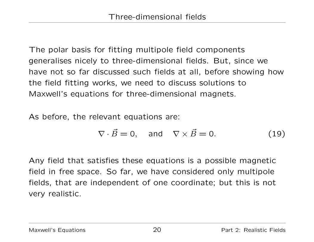
Three-dimensional fields
The polar basis for fitting multipole field components
generalises nicely to three-dimensional fields. But, since we
have not so far discussed such fields at all, before showing how
the field fitting works, we need to discuss solutions to
Maxwell’s equations for three-dimensional magnets.
As before, the relevant equations are:
∇ · ~B = 0, and ∇× ~B = 0. (19)
Any field that satisfies these equations is a possible magnetic
field in free space. So far, we have considered only multipole
fields, that are independent of one coordinate; but this is not
very realistic.
Maxwell’s Equations 20 Part 2: Realistic Fields
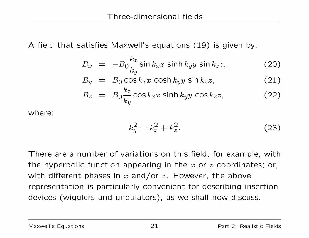
Three-dimensional fields
A field that satisfies Maxwell’s equations (19) is given by:
Bx = −B0kx
kysin kxx sinh kyy sin kzz, (20)
By = B0 cos kxx cosh kyy sin kzz, (21)
Bz = B0kz
kycos kxx sinh kyy cos kzz, (22)
where:
k2y = k2x + k2z . (23)
There are a number of variations on this field, for example, with
the hyperbolic function appearing in the x or z coordinates; or,
with different phases in x and/or z. However, the above
representation is particularly convenient for describing insertion
devices (wigglers and undulators), as we shall now discuss.
Maxwell’s Equations 21 Part 2: Realistic Fields
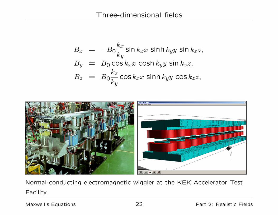
Three-dimensional fields
Bx = −B0kx
kysin kxx sinh kyy sin kzz,
By = B0 cos kxx cosh kyy sin kzz,
Bz = B0kz
kycos kxx sinh kyy cos kzz,
Normal-conducting electromagnetic wiggler at the KEK Accelerator Test
Facility.
Maxwell’s Equations 22 Part 2: Realistic Fields
Three-dimensional fields
If we take kx = 0, then the field becomes:
Bx = 0, (24)
By = B0 cosh kzy sin kzz, (25)
Bz = B0 sinh kzy cos kzz. (26)
The above equations describe a field that varies sinusoidally in
z, and has no horizontal (x) component at all. This is a field
that could only occur in an insertion device with infinite length,
and infinite width.
Maxwell’s Equations 23 Part 2: Realistic Fields
Three-dimensional fields
A better description would take account of the fact that the
longitudinal variation of the field will not be perfectly
sinusoidal. We can account for this by superposing fields with
different values of kz:
Bx = 0, (27)
By =∫B̃(kz) cosh kzy sin kzz dkz, (28)
Bz =∫B̃(kz) sinh kzy cos kzz dkz. (29)
We see that if we take measurements of By as a function of z
in the plane y = y0 (for fixed y0), then we can obtain the mode
coefficients B̃(kz) by a (discrete) Fourier transform.
This allows us to reconstruct all field components, at all
locations within the field.
Maxwell’s Equations 24 Part 2: Realistic Fields

Three-dimensional fields
Suppose we measure By at a set of locations z = z`, where:
z` =`
Nzmax, ` = −N,−N + 1,−N + 2, . . . , N. (30)
N is an integer, and the field has effectively fallen to zero atz = ±zmax.
We obtain the mode coefficients from:
B̃n =1
2N cosh(nkzy0)
N∑`=−N
By(z`) sin (nkzz`) , (31)
where kz = π/zmax.
And the field at any point can be reconstructed from:
By(y, z) =N∑
n=−NB̃n cosh (nkzy) sin (nkzz) , (32)
Bz(y, z) =N∑
n=−NB̃n sinh (nkzy) cos (nkzz) . (33)
Maxwell’s Equations 25 Part 2: Realistic Fields
Three-dimensional fields
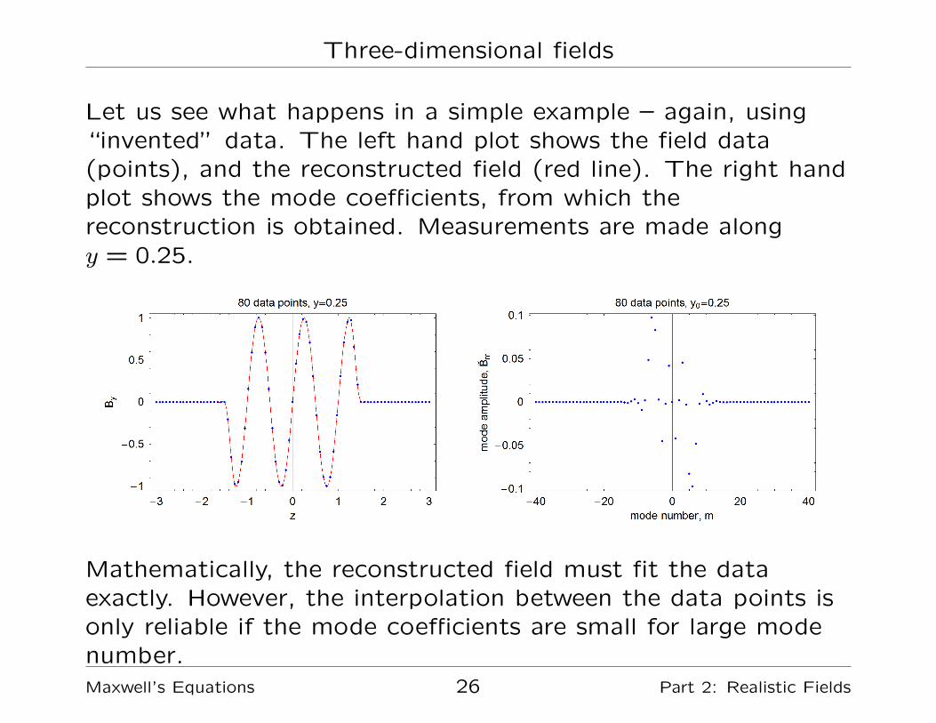
Let us see what happens in a simple example – again, using“invented” data. The left hand plot shows the field data(points), and the reconstructed field (red line). The right handplot shows the mode coefficients, from which thereconstruction is obtained. Measurements are made alongy = 0.25.
Mathematically, the reconstructed field must fit the dataexactly. However, the interpolation between the data points isonly reliable if the mode coefficients are small for large modenumber.Maxwell’s Equations 26 Part 2: Realistic Fields
Three-dimensional fields
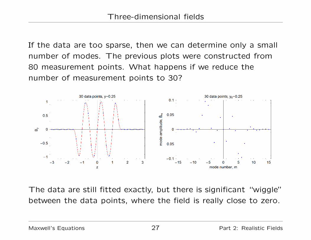
If the data are too sparse, then we can determine only a small
number of modes. The previous plots were constructed from
80 measurement points. What happens if we reduce the
number of measurement points to 30?
The data are still fitted exactly, but there is significant “wiggle”
between the data points, where the field is really close to zero.
Maxwell’s Equations 27 Part 2: Realistic Fields
Three-dimensional fields
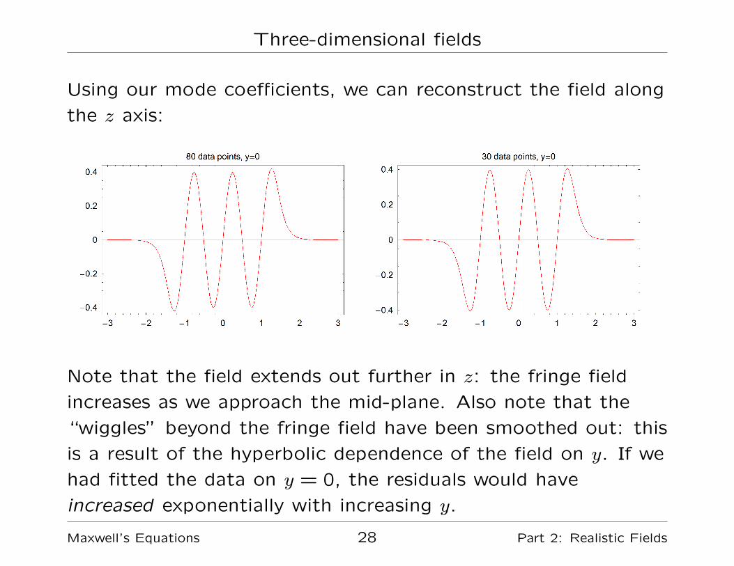
Using our mode coefficients, we can reconstruct the field along
the z axis:
Note that the field extends out further in z: the fringe field
increases as we approach the mid-plane. Also note that the
“wiggles” beyond the fringe field have been smoothed out: this
is a result of the hyperbolic dependence of the field on y. If we
had fitted the data on y = 0, the residuals would have
increased exponentially with increasing y.
Maxwell’s Equations 28 Part 2: Realistic Fields
Three-dimensional fields
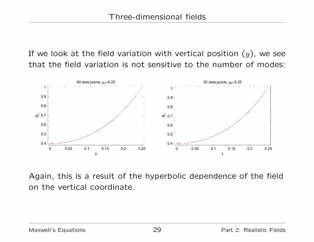
If we look at the field variation with vertical position (y), we see
that the field variation is not sensitive to the number of modes:
Again, this is a result of the hyperbolic dependence of the field
on the vertical coordinate.
Maxwell’s Equations 29 Part 2: Realistic Fields
Three-dimensional fields
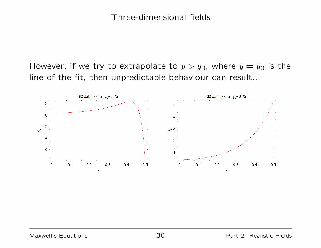
However, if we try to extrapolate to y > y0, where y = y0 is the
line of the fit, then unpredictable behaviour can result...
Maxwell’s Equations 30 Part 2: Realistic Fields
Three-dimensional fields
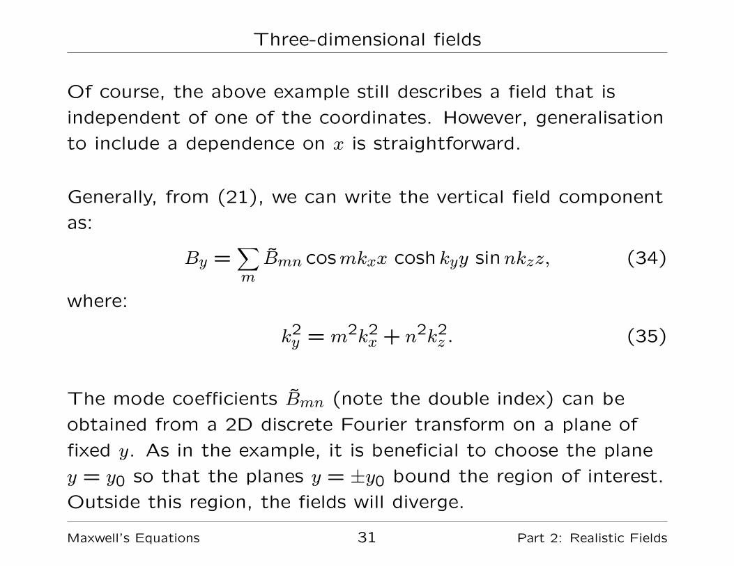
Of course, the above example still describes a field that is
independent of one of the coordinates. However, generalisation
to include a dependence on x is straightforward.
Generally, from (21), we can write the vertical field component
as:
By =∑mB̃mn cosmkxx cosh kyy sinnkzz, (34)
where:
k2y = m2k2x + n2k2z . (35)
The mode coefficients B̃mn (note the double index) can be
obtained from a 2D discrete Fourier transform on a plane of
fixed y. As in the example, it is beneficial to choose the plane
y = y0 so that the planes y = ±y0 bound the region of interest.
Outside this region, the fields will diverge.
Maxwell’s Equations 31 Part 2: Realistic Fields
Three-dimensional fields
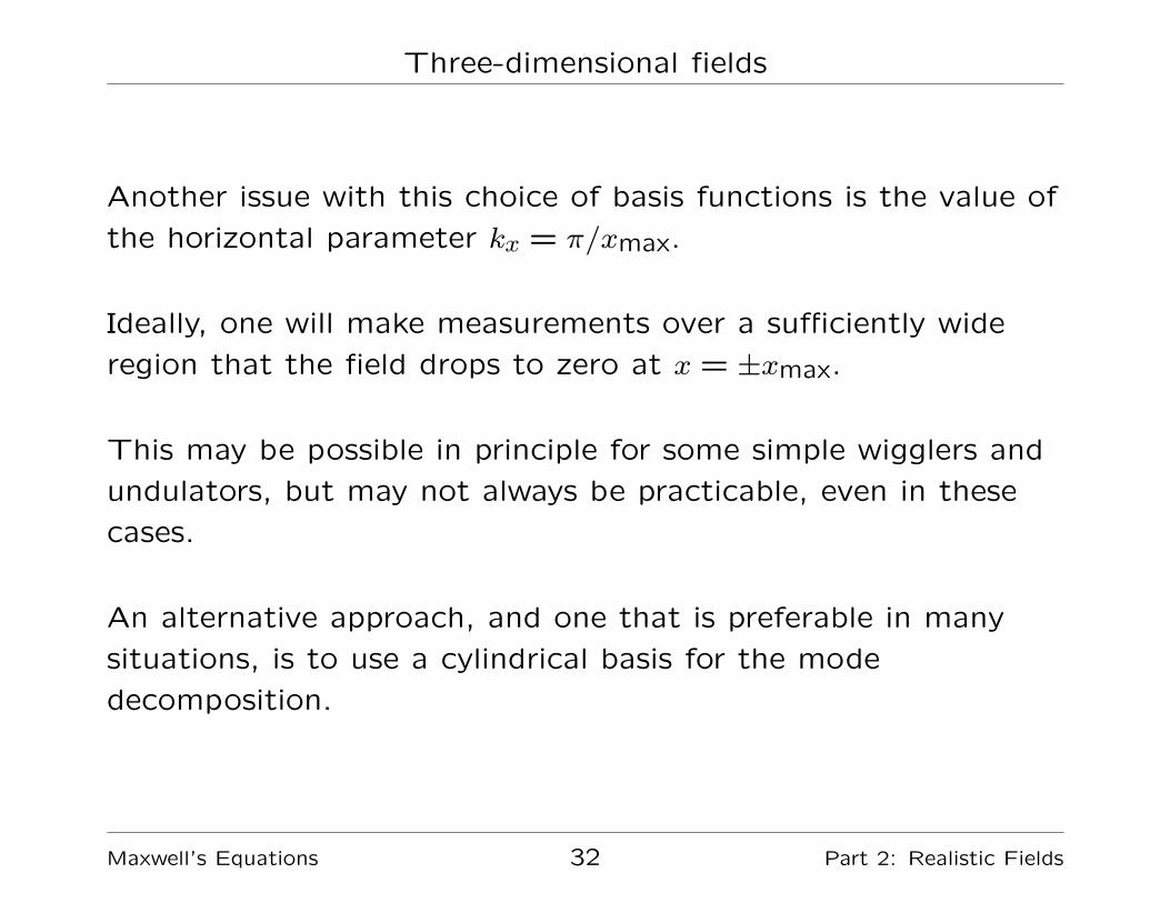
Another issue with this choice of basis functions is the value of
the horizontal parameter kx = π/xmax.
Ideally, one will make measurements over a sufficiently wide
region that the field drops to zero at x = ±xmax.
This may be possible in principle for some simple wigglers and
undulators, but may not always be practicable, even in these
cases.
An alternative approach, and one that is preferable in many
situations, is to use a cylindrical basis for the mode
decomposition.
Maxwell’s Equations 32 Part 2: Realistic Fields
Cylindrical basis functions for three-dimensional fields
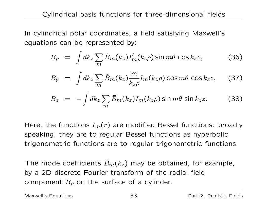
In cylindrical polar coordinates, a field satisfying Maxwell’s
equations can be represented by:
Bρ =∫dkz
∑mB̃m(kz)I
′m(kzρ) sinmθ cos kzz, (36)
Bθ =∫dkz
∑mB̃m(kz)
m
kzρIm(kzρ) cosmθ cos kzz, (37)
Bz = −∫dkz
∑mB̃m(kz)Im(kzρ) sinmθ sin kzz. (38)
Here, the functions Im(r) are modified Bessel functions: broadly
speaking, they are to regular Bessel functions as hyperbolic
trigonometric functions are to regular trigonometric functions.
The mode coefficients B̃m(kz) may be obtained, for example,
by a 2D discrete Fourier transform of the radial field
component Bρ on the surface of a cylinder.
Maxwell’s Equations 33 Part 2: Realistic Fields

Cylindrical basis functions for three-dimensional fields
We can draw a direct connection between the 3D polar basis,
and the multipole decomposition in 2D. We use the fact that
the modified Bessel functions have an expansion (for small ξ):
Im(ξ) =ξm
2mΓ(1 +m)+O(m+ 1). (39)
Therefore, if the mode coefficients are given by:
B̃m(kz) = 2mΓ(1 +m)Cmδ(kz)
mkm−1z
, (40)
where δ() is the Dirac delta function, then:
Bρ =∑mCmρ
m−1 sinmθ, (41)
Bθ =∑mCmρ
m−1 cosmθ, (42)
Bz = 0. (43)
Maxwell’s Equations 34 Part 2: Realistic Fields
Cylindrical basis functions for three-dimensional fields
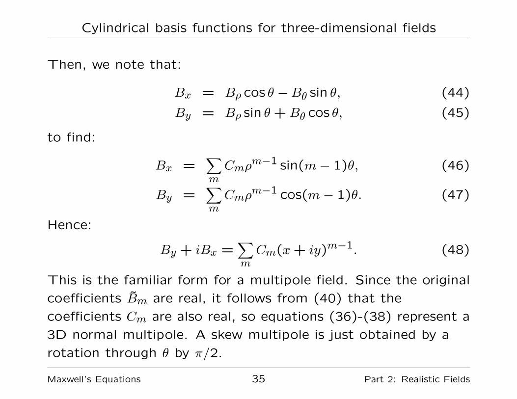
Then, we note that:
Bx = Bρ cos θ −Bθ sin θ, (44)
By = Bρ sin θ+Bθ cos θ, (45)
to find:
Bx =∑mCmρ
m−1 sin(m− 1)θ, (46)
By =∑mCmρ
m−1 cos(m− 1)θ. (47)
Hence:
By + iBx =∑mCm(x+ iy)m−1. (48)
This is the familiar form for a multipole field. Since the original
coefficients B̃m are real, it follows from (40) that the
coefficients Cm are also real, so equations (36)-(38) represent a
3D normal multipole. A skew multipole is just obtained by a
rotation through θ by π/2.
Maxwell’s Equations 35 Part 2: Realistic Fields
Cylindrical basis functions for three-dimensional fields
The connection between the 3D mode decomposition in the
cylindrical basis and the usual representation of a multipole
field gives us a nice interpretation of the mode coefficients B̃m.
The coefficient B̃m(kz) is essentially the longitudinal Fourier
amplitude of the 2m-pole field in the magnet. We should
remember, of course, that multipole fields only really exist in
infinitely long, uniform magnets. The representation (36)-(38),
however, can be used to describe realistic, 3D fields.
Maxwell’s Equations 36 Part 2: Realistic Fields
Cylindrical basis functions for three-dimensional fields
We mentioned above that the mode coefficients B̃m(kz) may
be obtained by a 2D discrete Fourier transform of the radial
field component Bρ on the surface of a cylinder.
As usual, it is beneficial to choose the radius of this cylinder to
be as large as possible: inside the cylinder, errors in the fit
decrease exponentially; outside the cylinder, the errors increase
exponentially.
With good field data, it is possible to achieve a very good fit.
As an example, the following slides show fits to a model for a
permanent magnet wiggler for the TESLA damping ring. The
(nominal, on-axis) peak field is 1.7T, and the wiggler period is
0.4 m. The fits were obtained using 18 azimuthal and 100
longitudinal modes, on a cylinder of radius 9mm.
Maxwell’s Equations 37 Part 2: Realistic Fields
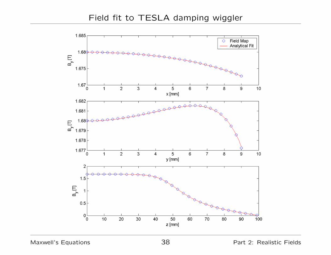
Field fit to TESLA damping wiggler
Maxwell’s Equations 38 Part 2: Realistic Fields
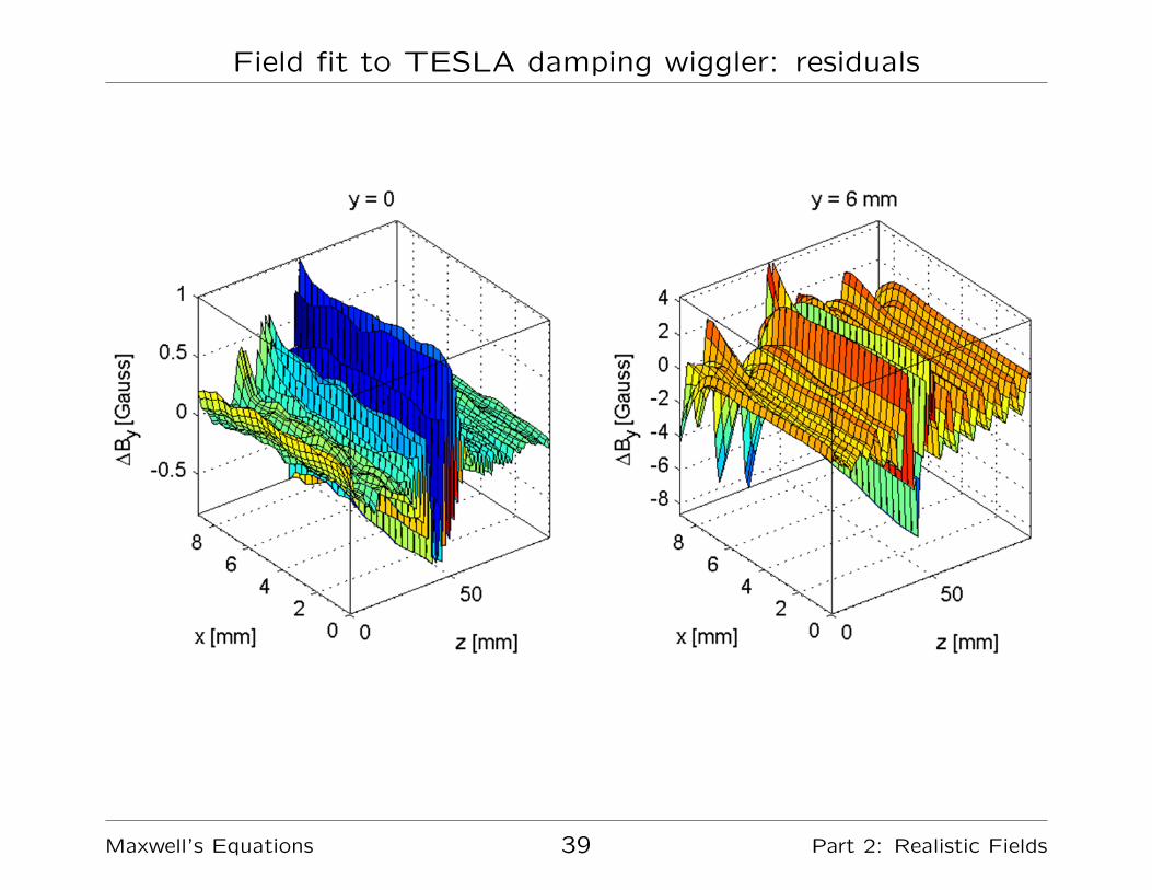
Field fit to TESLA damping wiggler: residuals
Maxwell’s Equations 39 Part 2: Realistic Fields
Final remarks
Often, the apertures in accelerator magnet (particularly, ininsertion devices) are not circular: the horizontal aperture iswider than the vertical. In such cases, a good fit can beobtained over a wider region by using an elliptical cross-sectionfor the cylinder, rather than a circular cross-section.
It is possible to perform an inverse Fourier transform on themode coefficients in the longitudinal dimension z, whileretaining the mode decomposition in θ. Then, we obtain arepresentation in which the “multipole component” appears asa function of z. This approach leads to the idea of generalisedgradients.
For further information on both these topics, see the book byAlex Dragt:
“Lie methods for nonlinear dynamics with applications toaccelerator physics.”http://www.physics.umd.edu/dsat/dsatliemethods.html
Maxwell’s Equations 40 Part 2: Realistic Fields

Summary of Lecture 1
Maxwell’s equations impose strong constraints on magnetic
fields that may exist.
The linearity of Maxwell’s equations means that complicated
fields may be expressed as a superposition of simpler fields.
In two dimensions, it is convenient to represent fields as a
superposition of multipole fields.
Multipole fields may be generated by sinusoidal current
distributions on a cylinder bounding the region of interest.
In regions without electric currents, the magnetic field may be
derived as the gradient of a scalar potential.
The scalar potential is constant on the surface of a material
with infinite permeability. This property is useful for defining
the shapes of iron poles in multipole magnets.
Maxwell’s Equations 41 Part 2: Realistic Fields
Summary of Lecture 2
Symmetries in multipole magnets restrict the multipolecomponents that can be present in the field.
It is useful to be able to find the multipole components in agiven field from numerical field data: but this must be donecarefully, if the results are to be accurate.
Usually, it is advisable to calculate multipole components usingfield data on a surface enclosing the region of interest: anyerrors or residuals will decrease exponentially within thatregion, away from the boundary. Outside the boundary,residuals will increase exponentially.
Techniques for finding multipole components in twodimensional fields can be generalised to three dimensions,allowing analysis of fringe fields and insertion devices.
In two or three dimensions, it is possible to use a Cartesianbasis for the field modes; but a polar basis is sometimes moreconvenient.Maxwell’s Equations 42 Part 2: Realistic Fields
Appendix: The vector potential
In lecture 1, we used a scalar potential for the magnetic field to
derive the shape for the pole face of a multipole magnet.
The scalar potential Φ is defined such that:
~B = −∇Φ. (49)
With this definition, the equation ∇× ~B = 0 is automatically
satisfied. The equation ∇ · ~B = 0 leads to Laplace’s equation
for the scalar potential:
∇2Φ = 0. (50)
Maxwell’s Equations 43 Part 2: Realistic Fields
Appendix: The vector potential
However, the scalar potential is only defined in the absence of
currents. More generally, we need to use a vector potential ~A.
In fact, in the most general case of time-dependent electric and
magnetic fields, we need both a scalar potential φ, and a vector
potential ~A:
~B = ∇× ~A, and ~E = −∇φ−∂ ~A
∂t. (51)
Some important methods for beam dynamics analysis use the
potentials φ and ~A, rather than the fields. It is therefore useful
to have expressions for the potentials corresponding to the
expressions for the fields we have derived in the main part of
these lectures.
Maxwell’s Equations 44 Part 2: Realistic Fields
Appendix: The vector potential
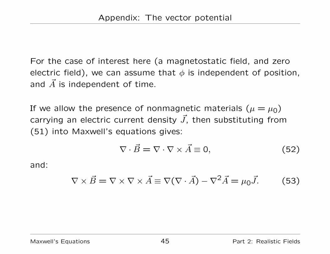
For the case of interest here (a magnetostatic field, and zero
electric field), we can assume that φ is independent of position,
and ~A is independent of time.
If we allow the presence of nonmagnetic materials (µ = µ0)
carrying an electric current density ~J, then substituting from
(51) into Maxwell’s equations gives:
∇ · ~B = ∇ · ∇ × ~A ≡ 0, (52)
and:
∇× ~B = ∇×∇× ~A ≡ ∇(∇ · ~A)−∇2 ~A = µ0~J. (53)
Maxwell’s Equations 45 Part 2: Realistic Fields
Appendix: The vector potential
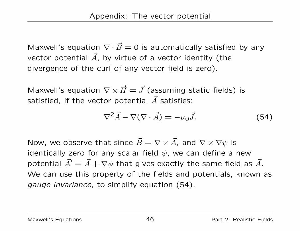
Maxwell’s equation ∇ · ~B = 0 is automatically satisfied by any
vector potential ~A, by virtue of a vector identity (the
divergence of the curl of any vector field is zero).
Maxwell’s equation ∇× ~H = ~J (assuming static fields) is
satisfied, if the vector potential ~A satisfies:
∇2 ~A−∇(∇ · ~A) = −µ0~J. (54)
Now, we observe that since ~B = ∇× ~A, and ∇×∇ψ is
identically zero for any scalar field ψ, we can define a new
potential ~A′ = ~A+∇ψ that gives exactly the same field as ~A.
We can use this property of the fields and potentials, known as
gauge invariance, to simplify equation (54).
Maxwell’s Equations 46 Part 2: Realistic Fields
Appendix: The vector potential
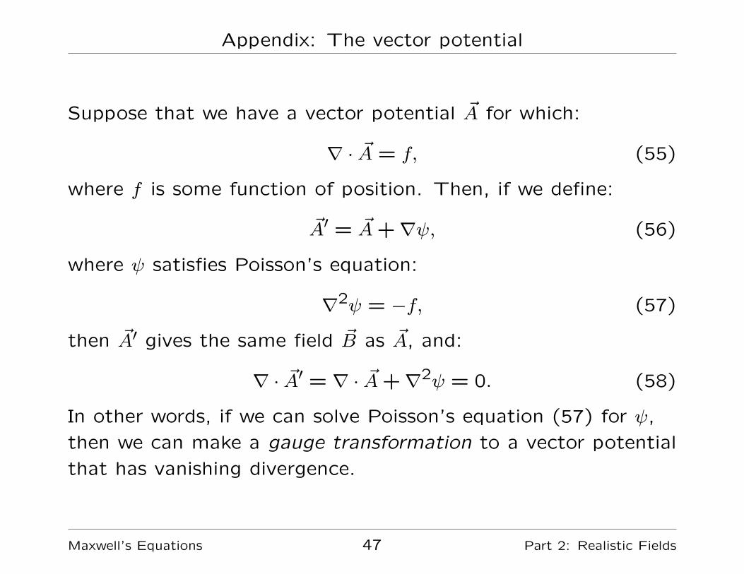
Suppose that we have a vector potential ~A for which:
∇ · ~A = f, (55)
where f is some function of position. Then, if we define:
~A′ = ~A+∇ψ, (56)
where ψ satisfies Poisson’s equation:
∇2ψ = −f, (57)
then ~A′ gives the same field ~B as ~A, and:
∇ · ~A′ = ∇ · ~A+∇2ψ = 0. (58)
In other words, if we can solve Poisson’s equation (57) for ψ,
then we can make a gauge transformation to a vector potential
that has vanishing divergence.
Maxwell’s Equations 47 Part 2: Realistic Fields

Appendix: The vector potential
Let us suppose that we find a vector potential that has
vanishing divergence:
∇ · ~A = 0. (59)
Equation (59) amounts to a condition that specifies a
particular choice of gauge: this particular choice (i.e. with zero
divergence) is known as the Coulomb gauge. It is useful,
because equation (54) for the vector potential then takes the
simpler form:
∇2 ~A = −µ0~J. (60)
This is Poisson’s equation, which has the standard solution:
~A(~r) = −µ0
4π
∫ ~J(~r ′)
|~r − ~r ′|d3r′. (61)
Maxwell’s Equations 48 Part 2: Realistic Fields
Appendix: The vector potential
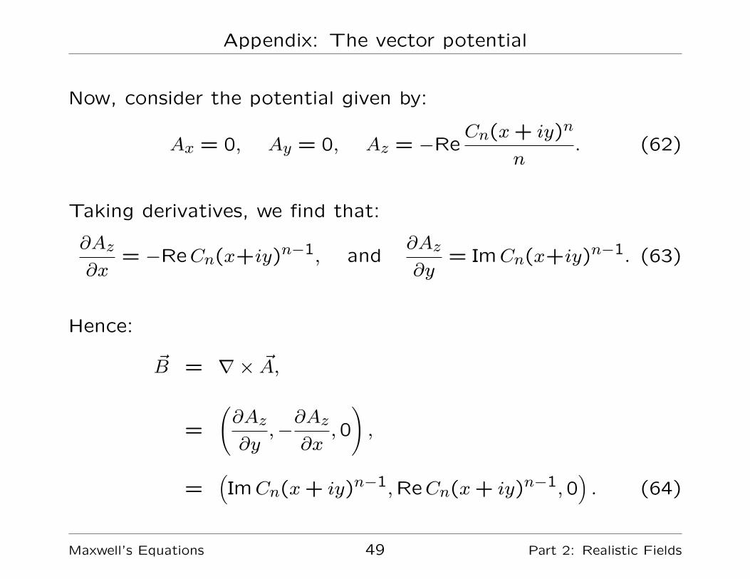
Now, consider the potential given by:
Ax = 0, Ay = 0, Az = −ReCn(x+ iy)n
n. (62)
Taking derivatives, we find that:
∂Az
∂x= −ReCn(x+iy)n−1, and
∂Az
∂y= ImCn(x+iy)n−1. (63)
Hence:
~B = ∇× ~A,
=
(∂Az
∂y,−∂Az
∂x,0
),
=(ImCn(x+ iy)n−1,ReCn(x+ iy)n−1,0
). (64)
Maxwell’s Equations 49 Part 2: Realistic Fields
Appendix: The vector potential
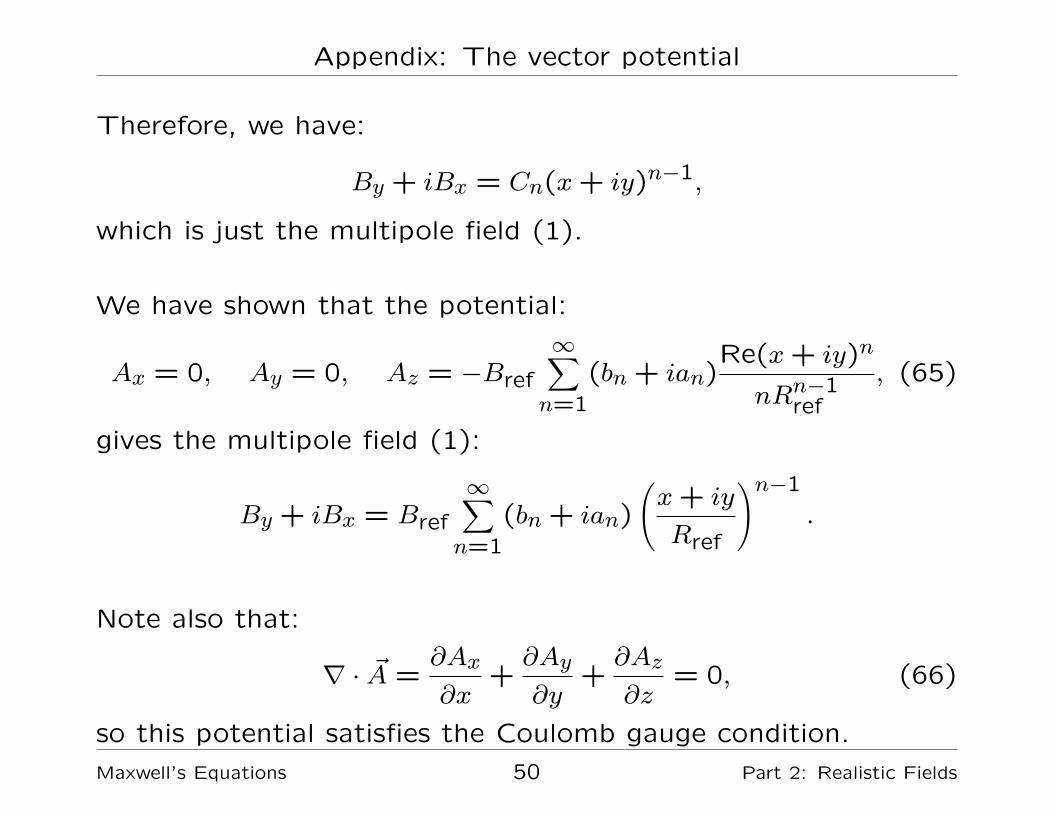
Therefore, we have:
By + iBx = Cn(x+ iy)n−1,
which is just the multipole field (1).
We have shown that the potential:
Ax = 0, Ay = 0, Az = −Bref
∞∑n=1
(bn + ian)Re(x+ iy)n
nRn−1ref
, (65)
gives the multipole field (1):
By + iBx = Bref
∞∑n=1
(bn + ian)
(x+ iy
Rref
)n−1
.
Note also that:
∇ · ~A =∂Ax
∂x+∂Ay
∂y+∂Az
∂z= 0, (66)
so this potential satisfies the Coulomb gauge condition.
Maxwell’s Equations 50 Part 2: Realistic Fields
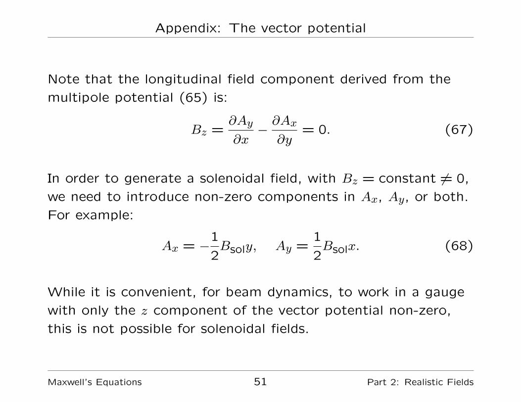
Appendix: The vector potential
Note that the longitudinal field component derived from the
multipole potential (65) is:
Bz =∂Ay
∂x−∂Ax
∂y= 0. (67)
In order to generate a solenoidal field, with Bz = constant 6= 0,
we need to introduce non-zero components in Ax, Ay, or both.
For example:
Ax = −1
2Bsoly, Ay =
1
2Bsolx. (68)
While it is convenient, for beam dynamics, to work in a gauge
with only the z component of the vector potential non-zero,
this is not possible for solenoidal fields.
Maxwell’s Equations 51 Part 2: Realistic Fields
Appendix: The vector potential
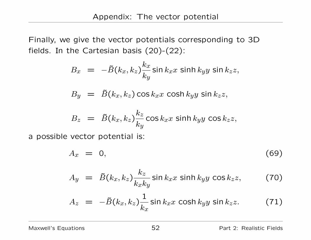
Finally, we give the vector potentials corresponding to 3D
fields. In the Cartesian basis (20)-(22):
Bx = −B̃(kx, kz)kx
kysin kxx sinh kyy sin kzz,
By = B̃(kx, kz) cos kxx cosh kyy sin kzz,
Bz = B̃(kx, kz)kz
kycos kxx sinh kyy cos kzz,
a possible vector potential is:
Ax = 0, (69)
Ay = B̃(kx, kz)kz
kxkysin kxx sinh kyy cos kzz, (70)
Az = −B̃(kx, kz)1
kxsin kxx cosh kyy sin kzz. (71)
Maxwell’s Equations 52 Part 2: Realistic Fields
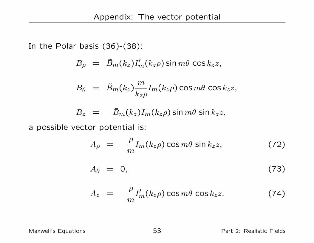
Appendix: The vector potential
In the Polar basis (36)-(38):
Bρ = B̃m(kz)I′m(kzρ) sinmθ cos kzz,
Bθ = B̃m(kz)m
kzρIm(kzρ) cosmθ cos kzz,
Bz = −B̃m(kz)Im(kzρ) sinmθ sin kzz,
a possible vector potential is:
Aρ = −ρ
mIm(kzρ) cosmθ sin kzz, (72)
Aθ = 0, (73)
Az = −ρ
mI ′m(kzρ) cosmθ cos kzz. (74)
Maxwell’s Equations 53 Part 2: Realistic Fields