Maxwell’s Equations

James Clerk Maxwell

(1831 - 1879)

November 9, 2001

∇ ·B(x, t) = 0, ∇×H(x, t) =4π

cJ(x, t) +

1

c

∂D(x, t)

∂t

∇× E(x, t) = −1

c

∂B(x, t)

∂t, ∇ ·D(x, t) = 4πρ(x, t)

Contents

1 Faraday’s Law of Induction 2

2 Energy in the Magnetic Field 7

2.1 Example: Motion of a permeable Bit in a Fixed J . . . . . . . . . . . 10

2.2 Energy of a Current distribution in an External Field . . . . . . . . . 12

3 Maxwell’s Displacement Current; Maxwell’s Equations 15

4 Vector and Scalar Potentials 17

5 Gauge Transformations 19

5.1 Lorentz Gauge . . . . . . . . . . . . . . . . . . . . . . . . . . . . . . . 19

5.2 Coulomb Transverse Gauge . . . . . . . . . . . . . . . . . . . . . . . 21

1

6 Green’s Functions for the Wave Equation 23

7 Derivation of Macroscopic Electromagnetism 28

8 Poynting’s Theorem; Energy and Momentum Conservation 28

8.1 Energy Conservation . . . . . . . . . . . . . . . . . . . . . . . . . . . 29

8.2 Momentum Conservation . . . . . . . . . . . . . . . . . . . . . . . . . 31

8.3 Need for Field Momentum . . . . . . . . . . . . . . . . . . . . . . . . 35

8.4 Example: Force on a Conductor . . . . . . . . . . . . . . . . . . . . . 36

9 Conservation Laws for Macroscopic Systems 37

10 Poynting’s Theorem for Harmonic Fields; Impedance, Admittance,

etc. 37

11 Transformations: Reflection, Rotation, and Time Reversal 42

11.1 Transformation Properties of Physical Quantities . . . . . . . . . . . 43

12 Do Maxwell’s Equations Allow Magnetic Monopoles? 48

A Helmholtz’ Theorem 50

2

Our first task in this chapter is to put time into the equations of electromagnetism.

There are traditionally two steps in this process. The first of them is to develop Fara-

day’s Law of Induction which is the culmination of a series of experiments performed

by Michael Faraday (1791 - 1867) around 1830. Faraday studied the current “in-

duced” in one closed circuit when a second nearby current-carrying circuit either was

moved or had its current varied as a function of time. He also did experiments in

which the second circuit was replaced by a permanent magnet in motion. The general

conclusion of these experiments is that if the “magnetic flux” through a closed loop

or circuit changes with time, an induced voltage or electromotive force (abbreviated

by Emf) appears in the circuit.

1 Faraday’s Law of Induction

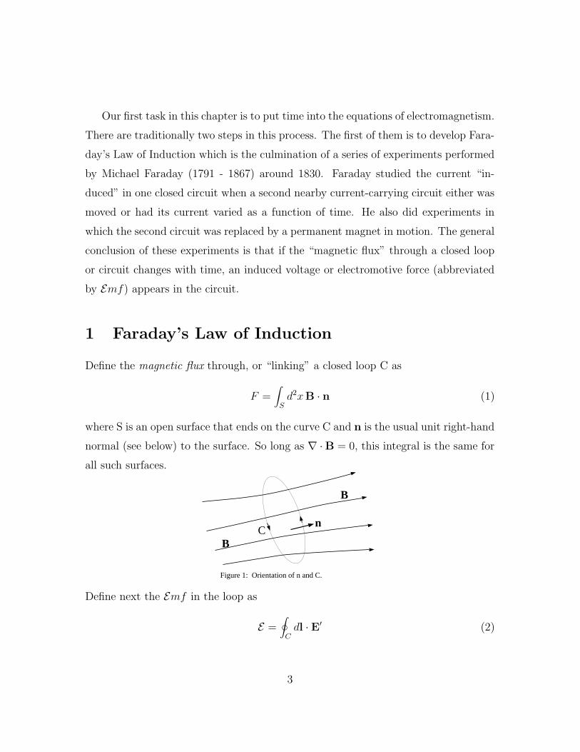
Define the magnetic flux through, or “linking” a closed loop C as

F =∫

Sd2xB · n (1)

where S is an open surface that ends on the curve C and n is the usual unit right-hand

normal (see below) to the surface. So long as ∇ ·B = 0, this integral is the same for

all such surfaces.

B

B

nC

Figure 1: Orientation of n and C.

Define next the Emf in the loop as

E =∮

Cdl · E′ (2)

3

where E′ is the electric field in that “frame of reference” in which the loop is at rest.1

The path C is traversed in such a direction that the unit normal n is the right-hand

normal relative to this direction. We may now write Faraday’s Law of Induction as

E = −kdFdt

(3)

where t is the time and k is a positive constant.

Let us make two points in relation to this equation.

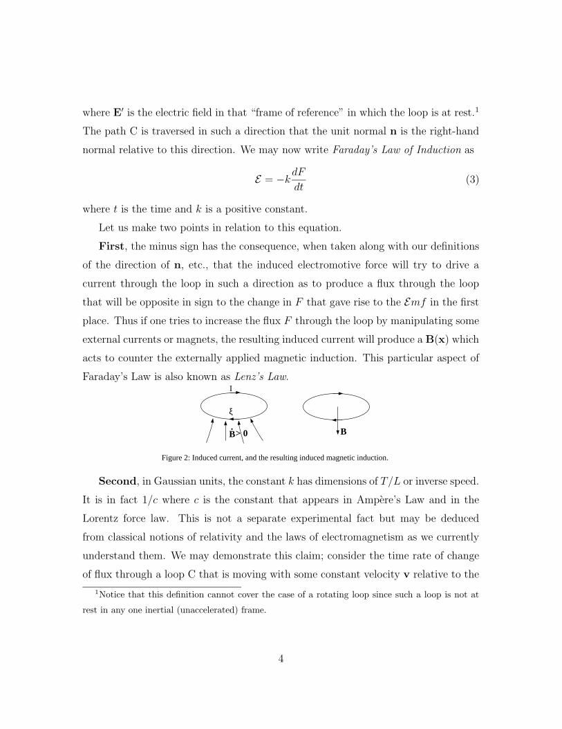
First, the minus sign has the consequence, when taken along with our definitions

of the direction of n, etc., that the induced electromotive force will try to drive a

current through the loop in such a direction as to produce a flux through the loop

that will be opposite in sign to the change in F that gave rise to the Emf in the first

place. Thus if one tries to increase the flux F through the loop by manipulating some

external currents or magnets, the resulting induced current will produce a B(x) which

acts to counter the externally applied magnetic induction. This particular aspect of

Faraday’s Law is also known as Lenz’s Law.

ξ

I

BB.

> 0

Figure 2: Induced current, and the resulting induced magnetic induction.

Second, in Gaussian units, the constant k has dimensions of T/L or inverse speed.

It is in fact 1/c where c is the constant that appears in Ampere’s Law and in the

Lorentz force law. This is not a separate experimental fact but may be deduced

from classical notions of relativity and the laws of electromagnetism as we currently

understand them. We may demonstrate this claim; consider the time rate of change

of flux through a loop C that is moving with some constant velocity v relative to the

1Notice that this definition cannot cover the case of a rotating loop since such a loop is not at

rest in any one inertial (unaccelerated) frame.

4

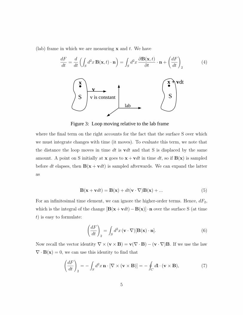
(lab) frame in which we are measuring x and t. We have

dF

dt=

d

dt

(∫

Sd2xB(x, t) · n

)=∫

Sd2x

∂B(x, t)

∂t· n +

(dF

dt

)

2

(4)

v

lab

x x + vdt

SS

Figure 3: Loop moving relative to the lab frame

v is constant

where the final term on the right accounts for the fact that the surface S over which

we must integrate changes with time (it moves). To evaluate this term, we note that

the distance the loop moves in time dt is vdt and that S is displaced by the same

amount. A point on S initially at x goes to x + vdt in time dt, so if B(x) is sampled

before dt elapses, then B(x + vdt) is sampled afterwards. We can expand the latter

as

B(x + vdt) = B(x) + dt(v · ∇)B(x) + ... (5)

For an infinitesimal time element, we can ignore the higher-order terms. Hence, dF2,

which is the integral of the change [B(x + vdt)−B(x)] ·n over the surface S (at time

t) is easy to formulate:

(dF

dt

)

2

=∫

Sd2x (v · ∇)[B(x) · n]. (6)

Now recall the vector identity ∇× (v×B) = v(∇ ·B)− (v · ∇)B. If we use the law

∇ ·B(x) = 0, we can use this identity to find that

(dF

dt

)

2

= −∫

Sd2xn · [∇× (v ×B)] = −

∮

Cdl · (v ×B), (7)

5

the last step following from Stokes theorem. Using Eqs. (4) and (7) in Faraday’s Law

of Induction2, we find

∮

Cdl · [E′ − k(v ×B)] = −k

∫

Sd2x

(∂B

∂t· n)

(8)

where E′ is the electric field in the frame where the loop is at rest; this frame moves

at velocity v relative to the one where B is measured (along with x and t).

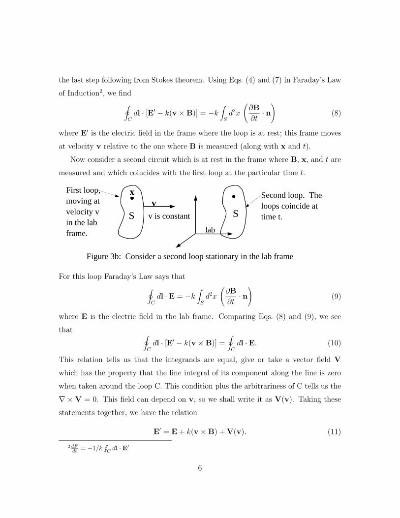
Now consider a second circuit which is at rest in the frame where B, x, and t are

measured and which coincides with the first loop at the particular time t.

v

lab

x

S

Figure 3b: Consider a second loop stationary in the lab frame

v is constant S

Second loop. Theloops coincide attime t.

First loop,moving atvelocity vin the labframe.

For this loop Faraday’s Law says that

∮

Cdl · E = −k

∫

Sd2x

(∂B

∂t· n)

(9)

where E is the electric field in the lab frame. Comparing Eqs. (8) and (9), we see

that ∮

Cdl · [E′ − k(v ×B)] =

∮

Cdl · E. (10)

This relation tells us that the integrands are equal, give or take a vector field V

which has the property that the line integral of its component along the line is zero

when taken around the loop C. This condition plus the arbitrariness of C tells us the

∇×V = 0. This field can depend on v, so we shall write it as V(v). Taking these

statements together, we have the relation

E′ = E + k(v ×B) + V(v). (11)

2 dFdt = −1/k

∮Cdl ·E′

6

This relation gives us the transformation of the electric field from the lab frame to

the rest frame of the moving circuit.

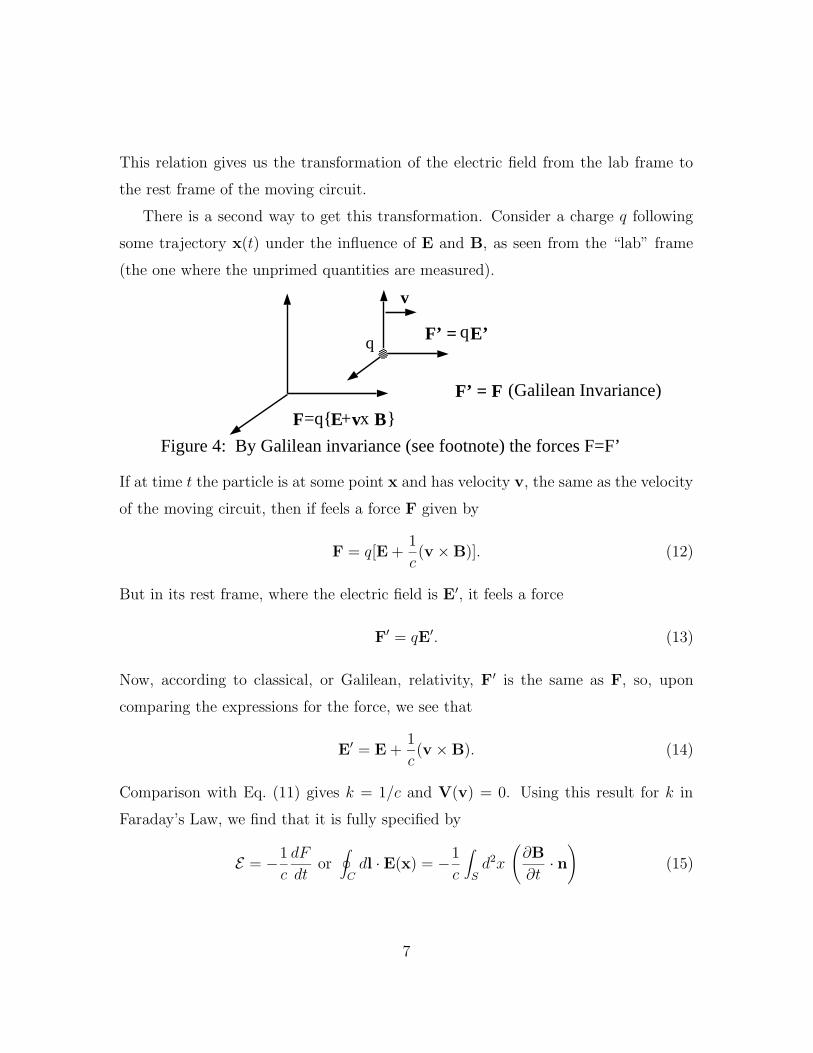
There is a second way to get this transformation. Consider a charge q following

some trajectory x(t) under the influence of E and B, as seen from the “lab” frame

(the one where the unprimed quantities are measured).

q

v

=q{ + x }F E v B

F’ = E’q

F’ = F (Galilean Invariance)

Figure 4: By Galilean invariance (see footnote) the forces F=F’

If at time t the particle is at some point x and has velocity v, the same as the velocity

of the moving circuit, then if feels a force F given by

F = q[E +1

c(v ×B)]. (12)

But in its rest frame, where the electric field is E′, it feels a force

F′ = qE′. (13)

Now, according to classical, or Galilean, relativity, F′ is the same as F, so, upon

comparing the expressions for the force, we see that

E′ = E +1

c(v ×B). (14)

Comparison with Eq. (11) gives k = 1/c and V(v) = 0. Using this result for k in

Faraday’s Law, we find that it is fully specified by

E = −1

c

dF

dtor

∮

Cdl · E(x) = −1

c

∫

Sd2x

(∂B

∂t· n)

(15)

7

for a stationary path.3 If we take the integral relation and apply Stokes theorem, we

find ∫

Sd2x

(∇× E +

1

c

∂B

∂t

)· n = 0. (16)

Because S is an arbitrary open surface, this relation must be true for all such surfaces.

That can only be if the integrand is everywhere zero, leading us to the differential

equation

∇× E(x, t) = −1

c

∂B(x, t)

∂t(17)

which is the differential equation statement of Faraday’s Law.

2 Energy in the Magnetic Field

Given Faraday’s Law, we are in a position to calculate the energy required to produce

a certain current distribution J starting from a state with J = 0 even though we

do not as yet know all of the time-dependent terms in the field equations. In this

section, we shall determine what is this energy. The mechanism that requires work

to be done is as follows: If we attempt to make a change in any existing current

distribution, there will be time-dependent sources (the current) with an accompanying

time-dependent magnetic induction. The latter must in turn produce electromagnetic

forces, or electric fields, against which work must be done not only in order to change

the currents but also simply in order to maintain them. By examining this work, we

can determine the change in the “magnetic energy” of the system.

To get started, consider a single loop or circuit carrying current I1. Given a

changing flux dF1/dt through this loop, there is an E1 = −c−1dF1/dt. If we wish

to maintain the current in the face of this electromotive force, we must counter the

latter by introducing an

3It should be remarked that all of this makes sense only to order v/c since in the next order,

v2/c2, Galilean relativity fails. However, the conclusion that k = 1/c must remain valid since k is a

constant (according to experiments), independent of the relative size of any velocities.

8

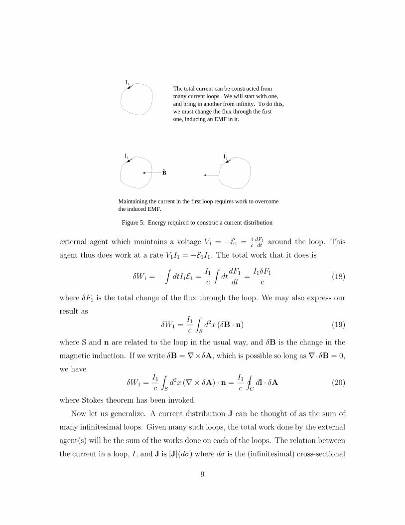
The total current can be constructed frommany current loops. We will start with one,and bring in another from infinity. To do this,we must change the flux through the firstone, inducing an EMF in it.

I1

I2I1

B.

Maintaining the current in the first loop requires work to overcomethe induced EMF.

Figure 5: Energy required to construc a current distribution

external agent which maintains a voltage V1 = −E1 = 1cdF1

dtaround the loop. This

agent thus does work at a rate V1I1 = −E1I1. The total work that it does is

δW1 = −∫dtI1E1 =

I1

c

∫dtdF1

dt=I1δF1

c(18)

where δF1 is the total change of the flux through the loop. We may also express our

result as

δW1 =I1

c

∫

Sd2x (δB · n) (19)

where S and n are related to the loop in the usual way, and δB is the change in the

magnetic induction. If we write δB = ∇×δA, which is possible so long as ∇·δB = 0,

we have

δW1 =I1

c

∫

Sd2x (∇× δA) · n =

I1

c

∮

Cdl · δA (20)

where Stokes theorem has been invoked.

Now let us generalize. A current distribution J can be thought of as the sum of

many infinitesimal loops. Given many such loops, the total work done by the external

agent(s) will be the sum of the works done on each of the loops. The relation between

the current in a loop, I, and J is |J|(dσ) where dσ is the (infinitesimal) cross-sectional

9

area of the loop. Thus Idl → Jdσdl or Jd3x. Integrating over individual loops and

summing over all loops is equivalent to integrating over all space, so we find that the

change in energy accompanying a change δA(x) in the vector potential (reflecting an

infinitesimal change δB(x) in the magnetic induction) is

δW =1

c

∫d3x [J(x) · δA(x)]. (21)

The change in the magnetic induction has to be infinitesimal for this expression to be

valid because we did not ask how the current density must be changed to produce it.

Note that this form indicates that W is a natural thermodynamic function function

of the potential or magnetic flux, rather than the sources

Now let us write the current density in terms of the fields. If we think we are

doing macroscopic electromagnetism, then4 J = c(∇×H)/4π and we can proceed as

follows:

δW =1

4π

∫

Vd3x [(∇×H) · δA] =

1

4π

∫

Vd3x [∇ · (H× δA) + H · (∇× δA)]

=1

4π

∮

Sd2x (H× δA) · n +

1

4π

∫

Vd3x (H · δB)

=1

4π

∫d3x (H · δB). (22)

The final step in this argument is achieved by letting the domain of integration be

all space and assuming that the fields H and δA fall off fast enough far away that

the surface integral vanishes. This is in fact true for a set of localized sources in the

limit that changes are made very slowly.

In the final step of our derivation we want to integrate δB up to some final B

starting from zero magnetic induction or zero current density. We can only do this

functional integral if we know how H depends on B. For a linear medium or set of

4This relation is only true for static phenomena; since we are changing the fields with time, it is

not valid. However, if the change is accomplished sufficiently slowly that ∂D∂t may be neglected, then

the corrections to Ampere’s Law are so small as to have negligible influence on our argument. Notice

too that use of this equation demands that changes in J(x) be done in such a way that ∇ · J = 0.

10

media, we know that

H · δB =1

2δ(H ·B) (23)

and so

δW =1

8π

∫d3x δ(B ·H) (24)

which integrates to

W =1

8π

∫d3xB(x) ·H(x) (25)

provided we define W ≡ 0 in the state with B ≡ 0.

Our result, Eq. (25), can be written in other forms; a particularly useful one is

obtained by writing B = ∇ × A and doing a parts integration in the familiar way.

Assuming that one can discard the resulting surface term (valid for localized sources),

we find

W =1

2c

∫d3xJ(x) ·A(x). (26)

In analogy with the electrostatic case, one conventionally defines the magnetic energy

density to be

w ≡ 1

8π(H(x) ·B(x)). (27)

2.1 Example: Motion of a permeable Bit in a Fixed J

Let us look at a specific example of the use of the expression(s) for the energy. Suppose

that there is some initial current distribution J0 which produces fields H0 and B0

and energy W0. Then we have

W0 =1

8π

∫d3xB0 ·H0 =

1

2c

∫d3xJ0 ·Ao. (28)

Now move some permeable materials around without changing the macroscopic cur-

rent density J0.

11

J(x)

µµ

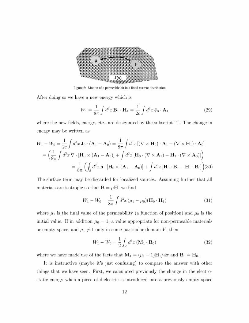
Figure 6: Motion of a permeable bit in a fixed current distribution

After doing so we have a new energy which is

W1 =1

8π

∫d3xB1 ·H1 =

1

2c

∫d3xJ0 ·A1 (29)

where the new fields, energy, etc., are designated by the subscript ‘1’. The change in

energy may be written as

W1 −W0 =1

2c

∫d3xJ0 · (A1 −A0) =

1

8π

∫d3x [(∇×H0) ·A1 − (∇×H1) ·A0]

=(

1

8π

∫d3x∇ · [H0 × (A1 −A0)] +

∫d3x [H0 · (∇×A1)−H1 · (∇×A0)]

)

=1

8π

(∮

Sd2xn · [H0 × (A1 −A0)] +

∫d3x [H0 ·B1 −H1 ·B0]

)(30)

The surface term may be discarded for localized sources. Assuming further that all

materials are isotropic so that B = µH, we find

W1 −W0 =1

8π

∫d3x (µ1 − µ0)(H0 ·H1) (31)

where µ1 is the final value of the permeability (a function of position) and µ0 is the

initial value. If in addition µ0 = 1, a value appropriate for non-permeable materials

or empty space, and µ1 6= 1 only in some particular domain V , then

W1 −W0 =1

2

∫

Vd3x (M1 ·B0) (32)

where we have made use of the facts that M1 = (µ1 − 1)H1/4π and B0 = H0.

It is instructive (maybe it’s just confusing) to compare the answer with other

things that we have seen. First, we calculated previously the change in the electro-

static energy when a piece of dielectric is introduced into a previously empty space

12

in the presence of some fixed charges. We found

W1 −W0 = −1

2

∫

Vd3xP1 · E0. (33)

The difference in sign between the electrostatic and magnetostatic energies is a reflec-

tion of the fact that in the magnetic system we maintained fixed currents and in the

electrostatic system, fixed charges. In the former case external agents must do work

to maintain the currents, and in the latter one, no work need be done to maintain the

fixed charges. Hence in the latter case, the force on the dielectric may be found by

using the argument that in a conservative system, the force is the negative gradient of

the energy (which is given above) with respect to the displacement of the dielectric.

If, in the magnetic system, the work done on the system by the current-maintaining

external agents turns out to be precisely twice as large as the change in the system’s

energy, then the force on the permeable material will be the (positive) gradient of the

energy with respect to the displacement of the material. This is, in fact, the case, as

we shall see below.

2.2 Energy of a Current distribution in an External Field

As a second example, consider the energy of a current distribution in an external

field.

W =1

c

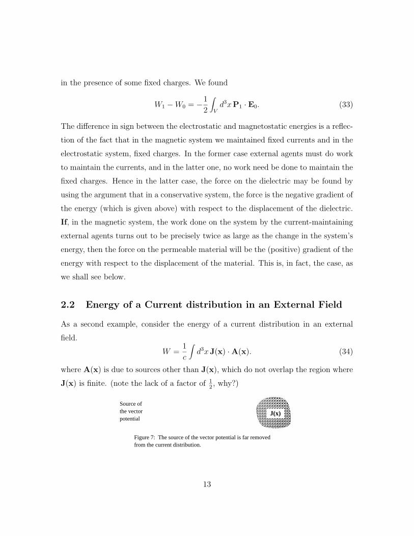
∫d3xJ(x) ·A(x). (34)

where A(x) is due to sources other than J(x), which do not overlap the region where

J(x) is finite. (note the lack of a factor of 12, why?)

J(x)

Source ofthe vectorpotential

Figure 7: The source of the vector potential is far removedfrom the current distribution.

13

Now assume that A(x) changes little over the region where J(x) is finite, and thus

expand A(x) about the origin of the current distribution.

A(x) = A(0) + x · ∇A(x)]x=0 + · · ·

through the now familiar manipulations, we end up with

W = m ·B(0) + · · ·

where m is the dipole moment of the current distribution

This appears to make no sense at all!! Recall last quarter, we found that the force

on a permanent dipole is

F = ∇(M ·B0)

which acts to minimize the potential −m ·B, rather than +m ·B!

I

m

B

F

F

Figure 8: Forces on a current loop.

Consider a current loop Clearly the force tries to make m and B parallel. Have

we misplaced a “-”-sign? Our expression for W is correct; however, we do not have a

conservative situation, since in calculating the force on the loop, we assumed that the

current I is constant. However, rotating the loop changes the flux through it which

induces an Emf which opposes the changing flux. Thus I will not be constant unless

external work is done to make it so. In such a non-conservative situation, the force is

not the negative gradient of the energy. For this particular situation, it must be that

the the force is given by the positive gradient of the energy.

To demonstrate that the last statement above is correct, we consider a set of

circuits Ci, i = 1, 2, ..., n, with currents Ii. The energy of this system is

W =1

2c

∫d3xJ ·A =

1

2c

∑

i

Ii

∮

Cidl ·A =

1

2c

∑

i

∫

Sid2xn · (∇×A)

14

=1

2c

∑

i

Ii

∫

Sid2x (n ·B) =

1

2c

∑

i

IiFi (35)

where Fi is the flux linking the ith circuit.

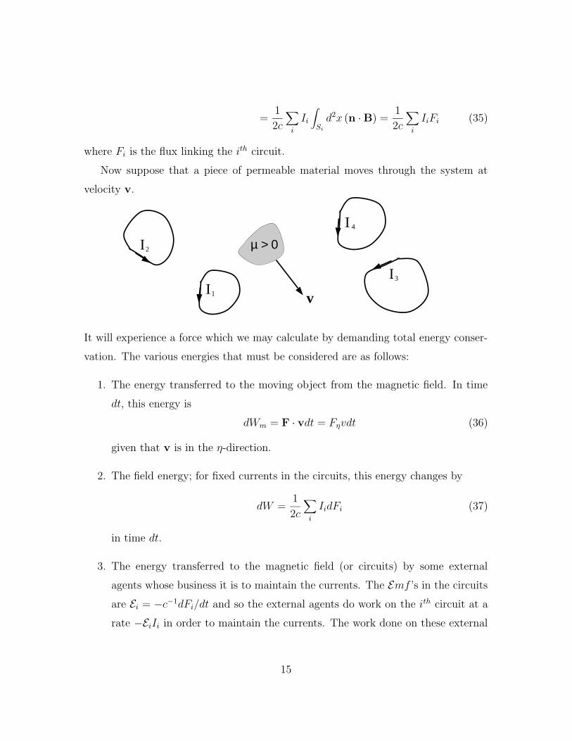
Now suppose that a piece of permeable material moves through the system at

velocity v.

µ > 0

v

I

I

II

1

2

3

4

It will experience a force which we may calculate by demanding total energy conser-

vation. The various energies that must be considered are as follows:

1. The energy transferred to the moving object from the magnetic field. In time

dt, this energy is

dWm = F · vdt = Fηvdt (36)

given that v is in the η-direction.

2. The field energy; for fixed currents in the circuits, this energy changes by

dW =1

2c

∑

i

IidFi (37)

in time dt.

3. The energy transferred to the magnetic field (or circuits) by some external

agents whose business it is to maintain the currents. The Emf ’s in the circuits

are Ei = −c−1dFi/dt and so the external agents do work on the ith circuit at a

rate −EiIi in order to maintain the currents. The work done on these external

15

agents in time dt is therefore

dWe =∑

i

EiIidt = −1

c

∑

i

IidFi = −2dW (38)

Now invoke conservation of energy which demands that the sum of all of the

preceding infinitesimal energy changes must be zero

dWm + dW + dWe = 0 (39)

or, using Eqs. (36) and (38),

Fηvdt = dW. (40)

Further, vdt = dη, so we find that

Fη = +

(∂W

∂η

)

J

(41)

as suggested earlier.

What would the force be if the flux F was held constant?

3 Maxwell’s Displacement Current; Maxwell’s Equa-

tions

Let us summarize the equations of electromagnetism as we now have them:

∇ ·B = 0

∇ ·D = 4πρ

∇×H =4π

cJ

∇× E = −1

c

∂B

∂t. (42)

These are not internally consistent. Consider the divergence of Ampere’s Law:

∇ · (∇×H) = 0 =4π

c(∇ · J) (43)

16

which implies that ∇ · J = 0. We know, however, that for general time-dependent

phenomena the divergence of the current density is not necessarily zero; indeed, we

have seen that charge conservation requires

∇ · J +∂ρ

∂t= 0. (44)

In consequence of this requirement, we must, at the very least, add a (time-dependent)

term to Ampere’s Law which will give, in distinction to Eq. (43),

∇ · (∇×H) =4π

c

[∇ · J +

∂ρ

∂t

]. (45)

This new term which must be a vector field X, has to be such that

∇ ·X =4π

c

∂ρ

∂t. (46)

We need not look beyond the things we have already learned to find a plausible

candidate for this term. We have a (static) equation which reads

ρ =1

4π∇ ·D; (47)

if we accept this as correct, we have

4π

c

∂ρ

∂t=

1

c

∂

∂t∇ ·D = ∇ ·

(1

c

∂D

∂t

). (48)

The simplest possible resolution of the inconsistency in the field equations is thus

to choose X to be c−1∂D/∂t, which would turn Ampere’s Law into the relation

∇×H =4π

cJ +

1

c

∂D

∂t. (49)

This adjustment was made5 by J. C. Maxwell in 1864, and the resulting set of differ-

ential field equations has since become known as Maxwell’s Equations:

∇ ·B(x, t) = 0, (50)

5He delivered a paper containing this statement in 1864, but he’d had the idea at least as early

as 1861.

17

∇ ·D(x, t) = 4πρ(x, t), (51)

∇× E(x, t) = −1

c

∂B(x, t)

∂t, (52)

and

∇×H(x, t) =4π

cJ(x, t) +

1

c

∂D(x, t)

∂t. (53)

The term that Maxwell added was called by him the displacement current JD:

JD ≡1

4π

∂D

∂t. (54)

This term has the appearance of an additional current entering Ampere’s Law so that

the latter reads

∇×H =4π

c(J + JD). (55)

Notice that ∇ · (J + JD) = 0. We shall not emphasize the “current” interpretation

of JD because it is misleading; the displacement current does not describe a flow of

charge and is not a true current density.

We close this section with two comments. First, the Maxwell equations must

be regarded as empirically justified. In the years since Maxwell’s final adjustment

of the field equations of electromagnetism, they have been subjected to extensive

experimental tests and have been found to be correct for classical phenomena (no

quantum effects or general relativistic effects); with proper interpretation, they even

have considerable validity within the realm of quantum phenomena. Second, the

equations as we have written them are for macroscopic electromagnetism. The more

fundamental version of these equations has B in place of H and E in place of D; then

the sources ρ and J are the total charge and current densities.

4 Vector and Scalar Potentials

For time-dependent phenomena, which are fully described by the Maxwell equations,

one can still write the fields E and B in terms of a scalar potential and a vector

18

potential. Because the divergence of the magnetic induction is still zero, one continues

to be able to find a vector potential A(x, t) which has the property that

B(x, t) = ∇×A(x, t); (56)

this potential is not unique. Further, since the curl of the electric field is not zero in

general, we cannot write E(x, t) as the gradient of a scalar; however, from Faraday’s

Law, Eq. (52), and from Eq. (56), we have

∇×(

E(x, t) +1

c

∂A(x, t)

∂t

)= 0 (57)

and so we can write the combination of fields in parentheses as the gradient of a scalar

function Φ(x, t):

E(x, t) +1

c

∂A(x, t)

∂t= −∇Φ(x, t) (58)

or

E(x, t) = −∇Φ(x, t)− 1

c

∂A(x, t)

∂t. (59)

Equations (56) and (59) tell us how to find B and E from potentials; these potentials

must themselves satisfy certain field equations that can be derived from the Maxwell

equations involving the sources ρ and J; the “homogeneous” or source-free equations

∇·B = 0 and∇×E = c−1∂B/∂t are then automatically satisfied. Letting H = B and

D = E for simplicity, we have, upon substituting Eqs. (56) and (59) into Eqs. (51)

and (53),

∇2Φ +1

c

∂

∂t(∇ ·A) = −4πρ (60)

and

∇× (∇×A) +1

c2

∂2A

∂t2+∇

(1

c

∂Φ

∂t

)=

4π

cJ. (61)

These equations clearly do not have particularly simple pleasing or symmetric forms.

However, we have some flexibility left in the choice of the potentials because we can

choose the vector potential’s divergence in an arbitrary fashion.

19

5 Gauge Transformations

Suppose that we have some A and Φ which give E and B correctly. Let us add to A

the gradient of a scalar function χ(x, t), thereby obtaining A′:

A′ ≡ A +∇χ. (62)

The field A′ has the same curl as A, and hence B = ∇×A′. However, the electric

field is not given by −∇Φ− c−1∂A′/∂t; we must therefore change Φ to Φ′ where Φ′

is chosen to that

E = −∇Φ′ − 1

c

∂A′

∂t. (63)

To this end we consider Φ′ = Φ + ψ where ψ is some scalar function of x and t. Our

requirement, Eq. (63), is that

E = −∇Φ−∇ψ − 1

c

∂A

∂t− 1

c

∂(∇χ)

∂t. (64)

However, we know that E is given according to Eq. (59), so, combining this relation

and Eq. (64), we find that ψ must satisfy the equation

∇ψ = −1

c

∂(∇χ)

∂t. (65)

A clear possible choice of ψ is ψ = −c−1∂χ/∂t.

What we have learned is that, given potentials A and Φ, we may make a gauge

transformation to equally acceptable potentials A′ and Φ′ given by

A′ = A +∇χ

Φ′ = Φ− 1

c

∂χ

∂t(66)

where χ(x, t) is an arbitrary scalar function of position and time.

5.1 Lorentz Gauge

Now let’s look again at the differential equations, Eqs. (60) and (61), for the poten-

tials; these may be written as

∇2Φ +1

c

∂

∂t(∇ ·A) = −4πρ

20

∇2A− 1

c2

∂2A

∂t2−∇

(∇ ·A +

1

c

∂Φ

∂t

)= −4π

cJ (67)

where we have used the identity ∇× (∇×A) = ∇(∇·A)−∇2A. These have a much

more pleasing form if A and Φ satisfy the Lorentz condition

∇ ·A +1

c

∂Φ

∂t= 0. (68)

Supposing for the moment that such a choice is possible, we make use of Eq. (68) in

Eq. (67) and find

∇2Φ− 1

c2

∂2Φ

∂t2= −4πρ

∇2A− 1

c2

∂2A

∂t2= −4π

cJ. (69)

These are very pleasing in that there are distinct equations for Φ and A, driven by

ρ and J, respectively; furthermore, all equations have the form of the classical wave

equation,

22ψ(x, t) = −4πf(x, t) (70)

where

22 ≡ ∇2 − 1

c2

∂2

∂t2(71)

is known as the D’Alembertian operator.

Consider next whether it is generally possible to find potentials that satisfy the

Lorentz condition. Suppose we have some potentials A0 and Φ0 for a given set of

sources J and ρ. We make a gauge transformation to new potentials A and Φ,

A = A0 +∇χ

Φ = Φ0 −1

c

∂χ

∂t, (72)

where the gauge function χ is to be chosen so that the Lorentz condition is satisfied

by the new potentials. The condition on χ is thus

0 = ∇ ·A +1

c

∂Φ

∂t= ∇ ·A0 +∇2χ+

1

c

∂Φ0

∂t− 1

c2

∂2χ

∂t2, (73)

21

or (∇2 − 1

c2

∂2

∂t2

)χ = −∇ ·A0 −

1

c

∂Φ0

∂t. (74)

The function that we seek is thus itself a solution of the classical wave equation with

a “source” which is, aside from some constant factor, just ∇ · A0 + c−1(∂Φ0/∂t).

Such a function always exists. In fact, there are many solutions to this wave equation

which means that there are many sets of potentials Φ and A which satisfy the Lorentz

condition. Potentials satisfying the Lorentz condition are said to be in the Lorentz

gauge.

5.2 Coulomb Transverse Gauge

Another gauge which can be useful is the Coulomb or transverse gauge. It is defined

by the condition that ∇ · A = 0. The beauty of this gauge is that in it the scalar

potential satisfies the Poisson equation,

∇2Φ(x, t) = −4πρ(x, t). (75)

We know the solution of this equation:

Φ(x, t) =∫d3x′

ρ(x′, t)

|x− x′| . (76)

Notice that the time is the same at both the source point x′ and the field point

x. There is nothing unacceptable about this because the scalar potential is not a

measurable quantity.

The vector potential in the Coulomb gauge is less satisfying; it obeys the wave

equation

22A = −4π

cJ +

1

c

∂

∂t(∇Φ). (77)

In practice one may solve for the potentials in the transverse gauge, given the

sources ρ and J, by first finding the scalar potential from the integral Eq. (76) and

then using the result in Eq. (77) and solving the wave equation (see the following

22

section). One should not be surprised to learn that the “source” term in Eq. (77)

involving the scalar potential can be made to look like a current; consider

1

c

∂

∂t(∇Φ) =

1

c

∂

∂t

[∇(∫

d3x′ρ(x′, t)

|x− x′|

)]= −∇

∫d3x′∇′ · J(x′, t)

|x− x′|

= −4π

c

(1

4π∇∫d3x′∇′ · J(x′, t)

|x− x′|

)(78)

The negative of the quantity within the parentheses (...) is called the longitudinal

current density. More generally, the longitudinal and transverse components Jl and

Jt of a vector field such as J are defined by the conditions6

Jl + Jt = J, ∇× Jl = 0, and ∇ · Jt = 0. (79)

In other words, Jl and Jt satisfy the equations

∇ · Jl = ∇ · J ∇ · Jt = 0

∇× Jl = 0 ∇× Jt = ∇× J,(80)

which means that Jl carries all of the divergence of the current density and Jt has all

of the curl.

From these equations and our knowledge of electrostatics we can see immediately

that

Jl(x, t) = − 1

4π∇(∫

d3x′∇′ · J(x′, t)

|x− x′|

)(81)

which may also be written as

Jl(x, t) = − 1

4π∇(∇ ·

∫d3x

J(x′, t)

|x− x′|

), (82)

and from that of magnetostatics we see that

Jt(x, t) = ∇×(

1

4π

∫d3x′∇′ × J(x′, t)

|x− x′|

)(83)

6In the appendix it is shown that such a decomposition, into longitudinal and transverse parts,

of a vector function of position is always possible

23

which may also be written as

Jt(x, t) = ∇×[

1

4π∇×

(∫d3x′

J(x′, t)

|x− x′|

)]. (84)

Comparison of Eq. (81) with Eqs. (77) and (76) shows that the wave equation for A

in the Coulomb or transverse gauge is

22A = −4π

c(J− Jl) = −4π

cJt. (85)

This equation lends justification to the term “transverse gauge.” In this gauge, the

vector potential is driven by the transverse part of the current in the same sense that

the vector potential is driven by the entire current in the Lorentz gauge.

6 Green’s Functions for the Wave Equation

We’re going to spend quite a lot of time looking for solutions of the classical wave

equation

22ψ(x, t) = −4πf(x, t); (86)

Therefore, it could be useful to have Green’s functions for the D’Alembertian operator,

meaning functions G(x, t; x′, t′) which satisfy the equation

22G(x, t; x′, t′) = −4πδ(x− x′)δ(t− t′) (87)

subject to some boundary conditions.

Compare this equation with that for the Green’s function for the Laplacian op-

erator, ∇2G(x,x′) = −4πδ(x − x′). The solution for the latter is, as we know,

G(x,x′) = 1/|x − x′| in an infinite space; physically, it is the scalar potential at x

produced by a unit point charge located at x′. The function G(x, t; x′, t′), by contrast

has dimensions 1/LT and may be thought of as the “response” at the space-time

point (x, t) to a unit “source” at the space-time point (x′, t′), that is, to a source

which exists only for a moment at a single space point. If this source is a pulse of

24

current or an evanescent point charge, then the Green’s function would be the vector

or scalar potential in the Lorentz gauge produced by that pulse.

As for the question of boundary conditions, we shall keep things as simple as

possible by considering an infinite system and applying the boundary condition that

G(x, t; x′, t′) → 0 for |x| → ∞. There is also a boundary condition on the behavior

of G(x, t; x′, t′) as a function of t; this is usually called an initial condition. We shall

not make any specific statement now of the initial conditions but will keep them in

mind as our derivation progresses.

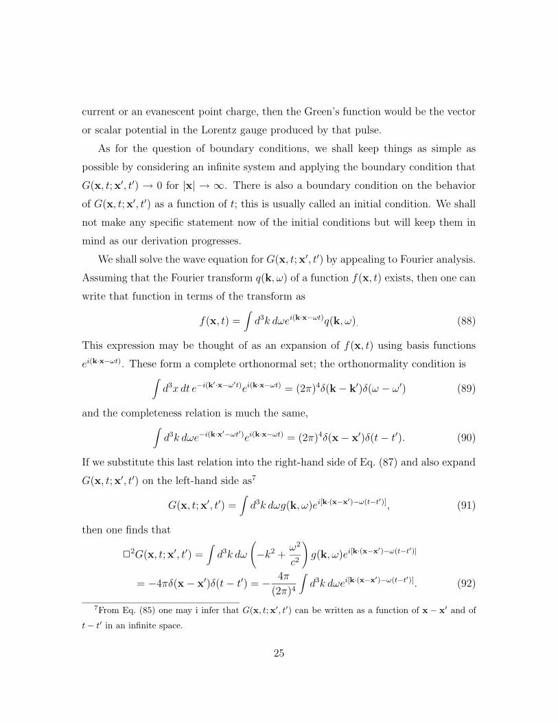
We shall solve the wave equation for G(x, t; x′, t′) by appealing to Fourier analysis.

Assuming that the Fourier transform q(k, ω) of a function f(x, t) exists, then one can

write that function in terms of the transform as

f(x, t) =∫d3k dωei(k·x−ωt)q(k, ω). (88)

This expression may be thought of as an expansion of f(x, t) using basis functions

ei(k·x−ωt). These form a complete orthonormal set; the orthonormality condition is∫d3x dt e−i(k

′·x−ω′t)ei(k·x−ωt) = (2π)4δ(k− k′)δ(ω − ω′) (89)

and the completeness relation is much the same,∫d3k dωe−i(k·x

′−ωt′)ei(k·x−ωt) = (2π)4δ(x− x′)δ(t− t′). (90)

If we substitute this last relation into the right-hand side of Eq. (87) and also expand

G(x, t; x′, t′) on the left-hand side as7

G(x, t; x′, t′) =∫d3k dωg(k, ω)ei[k·(x−x′)−ω(t−t′)], (91)

then one finds that

22G(x, t; x′, t′) =∫d3k dω

(−k2 +

ω2

c2

)g(k, ω)ei[k·(x−x′)−ω(t−t′)]

= −4πδ(x− x′)δ(t− t′) = − 4π

(2π)4

∫d3k dωei[k·(x−x′)−ω(t−t′)]. (92)

7From Eq. (85) one may i infer that G(x, t; x′, t′) can be written as a function of x − x′ and of

t− t′ in an infinite space.

25

The orthonormality of the basis functions may now be used to argue that the inte-

grands on the two sides of this equation must be equal; hence,

g(k, ω) =4π

(2π)4

1

k2 − ω2/c2. (93)

Now we have only to do the Fourier transform to find G(x, t; x′, t′). Consider first the

frequency integral,

I(k, t− t′) =∫ ∞

−∞dω

(e−iω(t−t′)

k2 − ω2/c2

). (94)

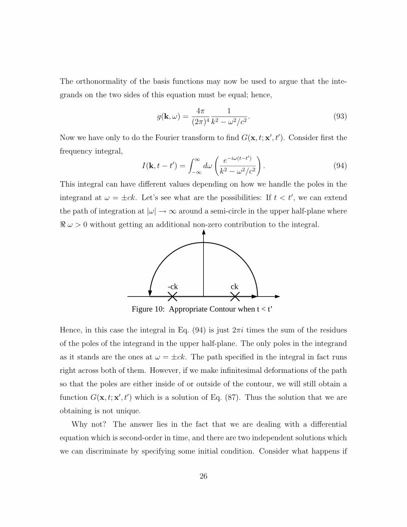
This integral can have different values depending on how we handle the poles in the

integrand at ω = ±ck. Let’s see what are the possibilities: If t < t′, we can extend

the path of integration at |ω| → ∞ around a semi-circle in the upper half-plane where

< ω > 0 without getting an additional non-zero contribution to the integral.

Figure 10: Appropriate Contour when t < t’

ck-ck

Hence, in this case the integral in Eq. (94) is just 2πi times the sum of the residues

of the poles of the integrand in the upper half-plane. The only poles in the integrand

as it stands are the ones at ω = ±ck. The path specified in the integral in fact runs

right across both of them. However, if we make infinitesimal deformations of the path

so that the poles are either inside of or outside of the contour, we will still obtain a

function G(x, t; x′, t′) which is a solution of Eq. (87). Thus the solution that we are

obtaining is not unique.

Why not? The answer lies in the fact that we are dealing with a differential

equation which is second-order in time, and there are two independent solutions which

we can discriminate by specifying some initial condition. Consider what happens if

26

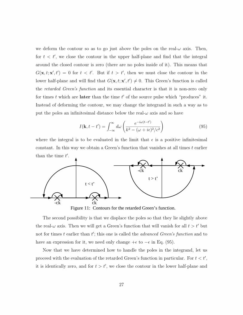
we deform the contour so as to go just above the poles on the real-ω axis. Then,

for t < t′, we close the contour in the upper half-plane and find that the integral

around the closed contour is zero (there are no poles inside of it). This means that

G(x, t; x′, t′) = 0 for t < t′. But if t > t′, then we must close the contour in the

lower half-plane and will find that G(x, t; x′, t′) 6= 0. This Green’s function is called

the retarded Green’s function and its essential character is that it is non-zero only

for times t which are later than the time t′ of the source pulse which “produces” it.

Instead of deforming the contour, we may change the integrand in such a way as to

put the poles an infinitesimal distance below the real-ω axis and so have

I(k, t− t′) =∫ ∞

−∞dω

(e−iω(t−t′)

k2 − (ω + iε)2/c2

)(95)

where the integral is to be evaluated in the limit that ε is a positive infinitesimal

constant. In this way we obtain a Green’s function that vanishes at all times t earlier

than the time t′.

t < t’

ck-ck

t > t’

ck-ck

Figure 11: Contours for the retarded Green’s function.

The second possibility is that we displace the poles so that they lie slightly above

the real-ω axis. Then we will get a Green’s function that will vanish for all t > t′ but

not for times t earlier than t′; this one is called the advanced Green’s function and to

have an expression for it, we need only change +ε to −ε in Eq. (95).

Now that we have determined how to handle the poles in the integrand, let us

proceed with the evaluation of the retarded Green’s function in particular. For t < t′,

it is identically zero, and for t > t′, we close the contour in the lower half-plane and

27

find

I(k, t− t′) = −c2∮

Cdω

e−iω(t−t′)

[ω − (ck − iε)][ω − (−ck − iε)]

= −c2(−2πi)

[e−ick(t−t′)

2ck+eick(t−t′)

−2ck

]=

2πc

ksin[ck(t− t′)]. (96)

Now we may complete the determination of G(x, t; x′, t′) by doing the integration

over the wavevector:

G(R, τ) =1

4π3

∫d3k

2πc

ksin(ckτ)eik·R (97)

where τ ≡ t− t′ and R ≡ (x− x′). Thus,

G(R, τ) =c

2π2

∫ ∞

0kdk

∫ 1

−1du∫ 2π

0dφ sin(ckτ)eikRu

=c

π

∫ ∞

0kdk

(eikR − e−ikR

ikR

)sin(ckτ)

= − c

4πR

∫ ∞

−∞dk(eikR − e−ikR

) (eickτ − e−ickτ

)

= − c

2R[δ(R + cτ) + δ(−R− cτ)− δ(R− cτ)− δ(−R + cτ)] =

δ(τ −R/c)R

; (98)

the final step here follows from the fact that this expression is only correct for τ > 0;

for τ < 0 G ≡ 0. In more detail, our result for the retarded Green’s function is

G(+)(x, t; x′, t′) =δ(t− t′ − |x− x′|/c)

|x− x′| . (99)

By similar manipulations one may show that the advanced Green’s function is

G(−)(x, t; x′, t′) =δ(t′ − t− |x− x′|/c)

|x− x′| . (100)

Given the appropriate Green’s function, we can write down a solution to the

classical wave equation with matching initial conditions and the appropriate boundary

conditions as |x| → ∞. Suppose that the wave equation is

22ψ(x, t) = −4πf(x, t); (101)

28

the solution is

ψ(x, t) =∫d3x′dt′G(x, t; x′, t′)f(x′, t′) (102)

as may be seen by operating on this equation with 22:

22ψ(x, t) =∫d3x′dt′22G(x, t; x′, t′)f(x′, t′)

=∫d3x′dt′[−4πδ(x− x′)δ(t− t′)]f(x′, t′) = −4πf(x, t). (103)

The fact that G(x, t; x′, t′) is proportional to a delta function means that one can

always complete the integration over time trivially. For the retarded Green’s function

in particular, one finds that

ψ(x, t) =∫d3x′

f(x′, t− |x− x′|/c)|x− x′| (104)

which has a fairly obvious interpretation.

Finally, it is worth pointing out that one may always add to ψ(x, t) a solution of

the homogeneous wave equation.

7 Derivation of Macroscopic Electromagnetism

Regretfully omitted because of time constraints.

8 Poynting’s Theorem; Energy and Momentum Con-

servation

A conservation law is a statement to the effect that some quantity q (such as charge)

is a constant for an isolated system. Often, it is possible to express the law mathe-

matically in the form

∇ · Jq +∂ρq∂t

=

(dρqdt

)

e

. (105)

29

Here, the density of the conserved quantity is ρq, its current density is Jq, and the

term on the right-hand side of the equation represents the contribution to the density

at a particular space-time point arising from external sources or sinks. As we have

already seen for the particular case of electrical charge, the divergence term represents

the flow of the conserved quantity away from a point in space while the partial time

derivative represents the rate at which its density is changing at that point. For

electrical charge, there are no (known) sources or sinks and so the term on the right-

hand side is zero.

8.1 Energy Conservation

It is possible to derive several such conservation laws from the Maxwell equations.

These include the charge conservation law8 and also ones that are interpreted as

energy, momentum, and angular momentum conservation. To get started, consider

the rate per unit volume at which the fields transfer energy to the charged particles,

or sources. The magnetic induction does no work since it is directed normal to the

velocity of a particle, and so we have only the electric field which does work a the

rate J · E per unit volume. This is, in the context of Eq. (105), the term −(dρ/dt)

representing the transfer of energy to external (to the fields) sources or sinks.

The total power Pm transferred to the sources within some domain V is found by

integrating over that domain,

Pm =∫

Vd3x (J · E). (106)

Now what we would like to do is perform some manipulations on J · E designed

to remove all reference to the current density, leaving only electromagnetic fields;

further, we want to make the expression look like the left-hand side of Eq. (105).

8Not surprising since the equations were explicitly constructed so as to be consistent with charge

conservation.

30

That is not so hard to do, starting with the generalization of Ampere’s law:

J · E =1

4π

[cE · (∇×H)− E · ∂D

∂t

]

=1

4π

[−c∇ · (E×H) + cH · (∇× E)− E · ∂D

∂t

]

= − c

4π∇ · (E×H)− 1

4π

(H · ∂B

∂t+ E · ∂D

∂t

). (107)

In the last step, Faraday’s law has been employed. The result is promising; there

is a divergence and the remainder is almost a time derivative. It becomes a time

derivative if the materials in the system have linear properties so that

H · ∂B

∂t=

1

2

∂

∂t(B ·H) and E · ∂D

∂t=

1

2

∂

∂t(E ·D). (108)

Then Eq. (107) becomes

−J · E =c

4π∇ · (E×H) +

1

8π

∂

∂t(E ·D + B ·H) (109)

which is of the very form we seek. The interpretation of this equation is that the

Poynting vector S, defined by

S ≡ c

4π(E×H) (110)

is the energy current density of the electromagnetic field and that the energy density

u, defined by

u ≡ 1

8π(E ·D + B ·H) (111)

is, indeed, the energy density of the electromagnetic field. In terms of these quantities

the conservation law is

−J · E = ∇ · S +∂u

∂t. (112)

Notice, however, that the energy current density is not unique. Because only its

divergence enters into the conservation law, we may add to S the curl of any vector

field and would still have Eq. (112). The distinction is not important for measurable

31

quantities because one always measures the rate of energy flow through a closed

surface (the surface of the detector),

∮

Sd2x (n · S) ≡

∫

Vd3x (∇ · S), (113)

so that only the divergence of S is important. Finally, note that if the conservation

law is integrated over some volume V, it can be expressed as

∫

Vd3x

∂u

∂t= −

∮

Sd2x (n · S)−

∫

Vd3x (J · E) (114)

with the interpretation that rate of change of field energy within the domain V is

equal to the rate at which field energy flows in through the surface of the domain

plus the rate at which the sources within V transfer energy to the field.

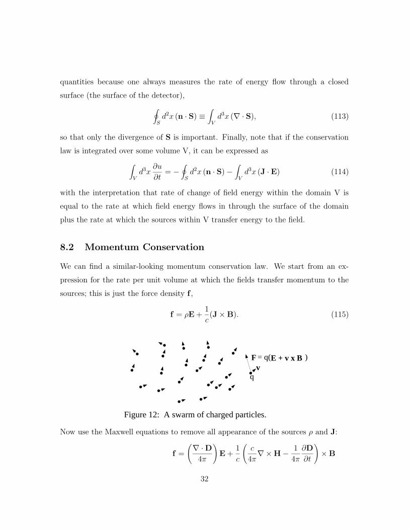
8.2 Momentum Conservation

We can find a similar-looking momentum conservation law. We start from an ex-

pression for the rate per unit volume at which the fields transfer momentum to the

sources; this is just the force density f ,

f = ρE +1

c(J×B). (115)

vF = q( )E + v x B

q

Figure 12: A swarm of charged particles.

Now use the Maxwell equations to remove all appearance of the sources ρ and J:

f =

(∇ ·D

4π

)E +

1

c

(c

4π∇×H− 1

4π

∂D

∂t

)×B

32

=1

4π

[E(∇ ·D) + (∇×H)×B− 1

c

(∂D

∂t×B

)]

=1

4π

[E(∇ ·D)−B× (∇×H)− 1

c

∂

∂t(D×B) +

1

c

(D× ∂B

∂t

)](116)

= − 1

4π

{1

c

∂(D×B)

∂t+ [B× (∇×H)−H(∇ ·B) + D× (∇× E)− E(∇ ·D)]

}

where we’ve used Faraday’s law and the field equation ∇ · B = 0. Now we have to

get all of the terms in the square brackets [...] in the final expression to look like a

divergence. There is one complication which is that the equation is a vector equation,

so we need a divergence which yields a vector, not a scalar.

Alternatively, we can look at Eq. (116) as three scalar equations, one for each

Cartesian component of the force density. Then the term in brackets contains three

components Ui and we want to write each component as the divergence of some vector

field Vi, Ui = ∇ ·Vi. If we expand the vector fields as

Vi =3∑

j=1

Vjiεj , (117)

with

Ui = ∇ ·Vi =∑

j

∂Vji∂xj

, (118)

then we have nine scalar functions Vji which can be put into a 3× 3 matrix. Let us

go a step further and define a dyadic V by its inner products with the complete set

of basis vectors εi:

εj · V · εi ≡ Vji. (119)

A convenient way to write V in terms of its components is

V =3∑

i,j=1

εjVjiεi, (120)

with the understanding that when an inner product is taken of V with a vector, the

dot product is taken with the left or right εi depending on whether the other vector

33

lies to the left or right of V. In particular,

∇ · V =∑

k

εk∂

∂xk

∑

i,j

εjVjiεi =∑

i,j

∂Vji∂xj

εi =∑

i

Uiεi. (121)

Now what we need, referring back to Eq. (116), is some V such that

∇ · V = B× (∇×H)−H(∇ ·B) + D× (∇× E)− E(∇ ·D) (122)

where we shall restrict ourselves to the case of vacuum, or at least constant µ and ε.

First, we have an identity,

B× (∇×B) =1

2∇(B ·B)− (B · ∇)B (123)

which allows us to write

B× (∇×H)−H(∇ ·B) =1

µ

[1

2∇(B ·B)− (B · ∇)B−B(∇ ·B)

]

=1

µ

∑

i,j

[1

2δijεj

∂B2

∂xi−Bi

∂Bj

∂xiεj −Bjεj

∂Bi

∂xi

]

=1

µ

∑

k

[εk

∂

∂xk

]·∑

i,j

εi

(1

2δijB

2 −BiBj

)εj

= ∇ ·∑

i,j

1

µεi

(1

2δijB

2 −BiBj

)εj

(124)

which is indeed the divergence of a dyadic. By similar means one may demonstrate

that

D× (∇× E)− E(∇ ·D) = ∇ ·∑

i,j

εεi

(1

2δijE

2 − EiEj)εj

. (125)

Putting these back into Eq. (124), we may write

−f =ε

4πc

∂

∂t[(E×B)]−∇ · T (126)

where the components Tij of the Maxwell stress tensor are

Tij ≡1

4π

[εEiEj +

1

µBiBj −

1

2δij

(εE2 +

1

µB2

)]. (127)

34

The Maxwell stress tensor is a symmetric tensor (in a uniform, isotropic, linear

medium) and has the physical interpretation that −Tij is the j-component of the

current density of the i-component of momentum. Note, however, that T is not

unique in that if we redefine it to include the curl of another dyadic, Eq. (116) would

still hold.

Let us define also a vector field g,

g ≡ 1

4πc(D×B) (128)

which is interpreted as the momentum density of the electromagnetic field, or the

momentum per unit volume. Notice that for D = εE and B = µH,

g =εµ

4πc(E×H) =

µε

c2S; (129)

there is thus a simple connection between the energy current density and the momen-

tum density of the field. Our conservation law is now simply written as

−f =∂g

∂t−∇ · T; (130)

if integrated over some domain V, it may also be expressed as

−∫

Vd3x f =

∫

Vd3x

∂g

∂t−∫

Sd2x (n · T). (131)

Finally, let us define

dPm

dt≡∫

Vd3x f and

dPf

dt≡∫

Vd3x

∂g

∂t; (132)

these are rather obviously meant to be the time rate of change of the mechanical

momentum9 and of the field momentum in V. Now we can write the conservation law

asdPm

dt+dPf

dt=∫

Sd2xn · T. (133)

9Note, however, that it includes only the rate of change of mechanical momentum as a consequence

of the forces applied to the particles by the electromagnetic field and does not include the change

in mechanical momentum which comes about because particles are entering and leaving the domain

V.

35

8.3 Need for Field Momentum

We defined our fields, the electric field and the magnetic induction, in terms of the

force and torque, respectively, that they inflict upon an elementary source. However,

as we have seen above, this definition is incomplete since the fields also carry energy

and momentum. From a quantum point of view, this is obvious since we can think

of the fields as resulting from the exchange of real and virtual photons each with

momentum hk and energy hω. However, from a 19’th century perspective the need

of the field to carry energy and momentum (especially momentum) is less obvious.

However, Newton’s law of action and reaction requires that the field carry mo-

mentum. First consider two completely isolated particles in free space. If the only

force exerted on either particle is from its counterpart, then the net momentum P is

conserved when the forces are equal and opposite.

dP

dt=

d

dt(P1 + P2) = m1

dv1

dt+m2

dv2

dt= F1 + F2

I.e. the momentum is conserved when F1 = −F2

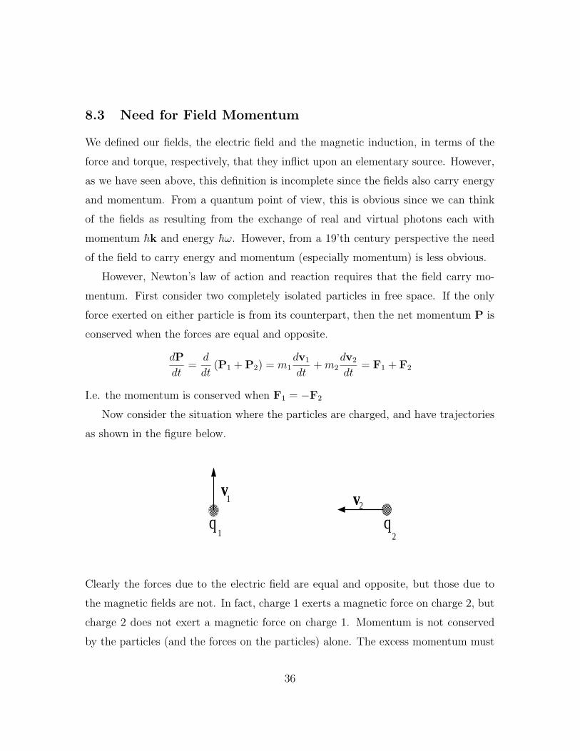
Now consider the situation where the particles are charged, and have trajectories

as shown in the figure below.

q q1 2

vv1

2

Clearly the forces due to the electric field are equal and opposite, but those due to

the magnetic fields are not. In fact, charge 1 exerts a magnetic force on charge 2, but

charge 2 does not exert a magnetic force on charge 1. Momentum is not conserved

by the particles (and the forces on the particles) alone. The excess momentum must

36

be carried by the field! Thus, the field is required to have a momentum density by

Newtonian law.

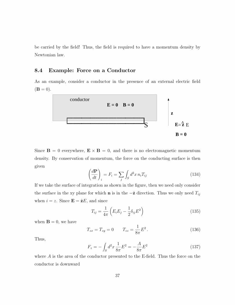
8.4 Example: Force on a Conductor

As an example, consider a conductor in the presence of an external electric field

(B = 0).

conductorE = 0 B = 0

z

E z= E

B = 0

S

Since B = 0 everywhere, E × B = 0, and there is no electromagnetic momentum

density. By conservation of momentum, the force on the conducting surface is then

given (dP

dt

)

i

= Fi =∑

j

∫

Sd2xniTij (134)

If we take the surface of integration as shown in the figure, then we need only consider

the surface in the xy plane for which n is in the −z direction. Thus we only need Tij

when i = z. Since E = zE, and since

Tij =1

4π

(EiEj −

1

2δijE

2)

(135)

when B = 0, we have

Tzx = Tzy = 0 Tzz =1

8πE2 . (136)

Thus,

Fz = −∫

Sd2x

1

8πE2 = − A

8πE2 (137)

where A is the area of the conductor presented to the E-field. Thus the force on the

conductor is downward

37

9 Conservation Laws for Macroscopic Systems

Regretfully omitted.

10 Poynting’s Theorem for Harmonic Fields; Impedance,

Admittance, etc.

Poynting’s theorem has many important applications at the practical (electrical en-

gineering) level. In this section we briefly make a foray into such an application. We

shall restrict attention to harmonic fields which means ones that are harmonic (sine)

functions of time. To this end we write the time-dependent part of the fields, as well

as the sources, as e−iωt where ω is the angular frequency, and the physical field or

source so represented is the real part of the complex mathematical function that we

are using. For example,

E(x, t) = <[E(x)e−iωt

]≡ 1

2

[E(x)e−iωt + E∗(x)eiωt

]. (138)

Similarly,

J(x, t) · E(x, t) =1

4

[J(x)e−iωt + J∗(x)eiωt

]·[E(x)e−iωt + E∗(x)eiωt

](139)

=1

2<[J∗(x) · E(x) + J(x) · E(x)e−2iωt

].

The time-average of the product is particularly simple; the term which varies as e−2iωt

has a zero time-average and so we are left with

< J(x, t) · E(x, t) >=1

2< [J∗(x) · E(x)] . (140)

One can easily see that there is a general rule for the time-average of the product

of two harmonic functions. Given Q(x, t) and R(x, t),

Q(x, t) = <[Q(x)e−iωt

]R(x, t) = <

[R(x)e−iωt

], (141)

38

the time average of the product may be expressed as

< Q(x, t)R(x, t) >=1

2< [R∗(x)Q(x)] =

1

2< [R(x)Q∗(x).] (142)

We start by supposing that all fields are harmonic. Then they all have the complex

form F(x)e−iωt and they all have time derivatives give by

∂(F(x)e−iωt)

∂t= −iωF(x)e−iωt (143)

so that the Maxwell equations for the complex amplitudes (just the position-dependent

parts of the fields) are

∇ ·B(x) = 0 ∇× E(x)− iωc

B(x)

∇ ·D(x) = 4πρ(x) ∇×H(x) + iω

cD(x) =

4π

cJ(x). (144)

Notice that there is no problem in generalizing the Maxwell equations to complex

fields because the equations involve linear combinations, with real coefficients, of

complex objects. One thus has two sets of equations, one for the real parts of these

objects and one for the imaginary parts. The set for the real parts comprises the

“true” Maxwell equations.

For the remainder of this section, the symbols E, B, etc, stand for the complex

amplitudes E(x), B(x), ... . We can rederive the Poynting theorem for these by

starting from the inner product J∗ · E and proceeding as in the original derivation.

The result is

J∗ · E =c

4π

[−∇ · (E×H∗)− iω

c(E ·D∗ −B ·H∗)

]. (145)

Define now the (complex) Poynting vector and energy densities

S ≡ c

8π(E×H∗), (146)

and

we ≡1

16π(E ·D∗) wm ≡

1

16π(B ·H∗). (147)

39

Notice that the real part of S is just the time-averaged real Poynting vector while

the real parts of the energy densities are the time-averaged energy densities. More

generally, the energy densities can be complex functions, depending on the relations

between D and E and between B and H. If the two members of each pair of fields are

in phase with one another, then the corresponding energy density is real. Similarly,

if E and H are in phase, then S is also real.

In terms of our densities, Poynting’s theorem for harmonic fields becomes

1

2J∗ · E = −∇ · S− 2iω(we − wm). (148)

If we integrate this expression over some domain V and apply the divergence theorem

to the term involving the Poynting vector, we find the relation

1

2

∫

Vd3xJ∗ · E + 2iω

∫

Vd3x (we − wm) +

∮

Sd2xS · n = 0. (149)

The interpretation of this equation is that the real part expresses the time-averaged

conservation of energy. The imaginary part also has a meaning in connection with

energy and its flow.

Consider first the simplest case of real we and wm. Then the energy densities drop

out of the real part of this equation and what it (the real part) tells us is that the

time-average rate of doing work on the sources in V is equal to the time-averaged

flow of energy (expressed by the Poynting vector) into V through the surface S. If

the energy densities are not real, then there is an additional real piece in Eq. (149)

so that the work done on the sources in V is not equal to the energy that comes in

through S; this case corresponds to having “lossy” materials within V which dissipate

additional energy.

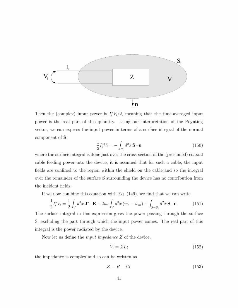
Now let’s suppose that there is some electromagnetic device within V, i.e., sur-

rounded by S. Let it have two input terminals which are its only material communi-

cation with the rest of the world. At these terminals there are some input current Ii

and voltage Vi which we suppose are harmonic and which may also be written in the

form Eq. (138).

40

V

Ii

i

iS

n

Z V

Then the (complex) input power is I∗i Vi/2, meaning that the time-averaged input

power is the real part of this quantity. Using our interpretation of the Poynting

vector, we can express the input power in terms of a surface integral of the normal

component of S,1

2I∗i Vi = −

∫

Sid2xS · n (150)

where the surface integral is done just over the cross-section of the (presumed) coaxial

cable feeding power into the device; it is assumed that for such a cable, the input

fields are confined to the region within the shield on the cable and so the integral

over the remainder of the surface S surrounding the device has no contribution from

the incident fields.

If we now combine this equation with Eq. (149), we find that we can write

1

2I∗i Vi =

1

2

∫

Vd3xJ∗ · E + 2iω

∫

Vd3x (we − wm) +

∫

S−Sid2xS · n. (151)

The surface integral in this expression gives the power passing through the surface

S, excluding the part through which the input power comes. The real part of this

integral is the power radiated by the device.

Now let us define the input impedance Z of the device,

Vi ≡ ZIi; (152)

the impedance is complex and so can be written as

Z ≡ R− iX (153)

41

where the resistance R and the reactance X are real. From Eq. (151) we find expres-

sions for these:

R =1

|Ii|2{Re

[∫

Vd3xJ∗ · E + 2

∫

S−Sid2xS · n

]+ 4ωIm

[∫

Vd3x (wm − we)

]}(154)

and

X =1

|Ii|2{

4ωRe[∫

Vd3x (wm − we)

]− Im

[∫

Vd3xJ∗ · E + 2

∫

S−Sid2xS · n

]}.

(155)

By deforming the surface so that it lies far away from the device, one may make the

integral over S · n purely real so that it does not contribute to the reactance; then it

is only a part of the resistance and is the so-called “radiation resistance” which will

be present if the device radiates a significant amount of power.

Our result has a simple and pleasing form at low frequencies. Then radiation

is negligible and so the contributions of the surface integral may be ignored. Also,

we may drop the term in the resistance proportional to ω. Then, assuming the

current density and electric field are related by J = σE where σ is the (real) electrical

conductivity, and assuming real energy densities, we find

R =1

|Ii|2∫

Vd3xσ|E|2 (156)

and

X =4ω

|Ii|2∫

Vd3x (wm − we) (157)

The last equation may be used to established contact between our expressions, based

on the electromagnetic field equations, and some standard and fundamental relations

in elementary circuit theory. If there is an inductance (magnetic energy-storing de-

vice) in the “black-box,” then the integral of the magnetic energy may be expressed

(see the first two or three problems at the end of Chap. 6 of Jackson) as ÃL|Ii|2/4, and

so we find the familiar (if one knows anything about circuits) result that X = Lω. But

if there is a capacitor, the energy becomes |Qi|2/4C where the charge Qi is obtained

by integrating the current over time; that gives |Qi|2 = |Ii|2/ω2 and so X = −1/ωC,

another familiar tenet of elementary circuit theory.

42

11 Transformations: Reflection, Rotation, and Time

Reversal

Before entering into discussion of the specific transformations of interest, we give a

brief review of orthogonal transformations. Introduce a 3× 3 matrix a with compo-

nents aij and use it to transform a position vector x = (x1, x2, x3) = (x, y, z) into a

new vector x′:

x′i =∑

j

aijxj. (158)

An orthogonal transformation is one that leaves the length of the vector unchanged,

∑

i

(x′i)2 =

∑

i

x2i . (159)

Using this condition, one may show that a must satisfy the conditions

∑

i

aijaik = δjk (160)

and

det(a) = ±1. (161)

Orthogonal transformations with det(a) = +1 are simple rotations. The other ones

are combinations of a rotation and an inversion10; these are called improper rotations.

It is common to refer to a collection of three objects ψi, i = 1, 2, 3, which

transform, under orthogonal transformations, in the same way as the components

of x, as a vector, a polar vector, or a rank-one tensor. A collection of nine objects

qij, i, j = 1, 2, 3, which transform in the same way as the nine objects xixj is called a

rank-two tensor. And so on. An object which is invariant, that is, which is unchanged

under an orthogonal transformation, is called a scalar or rank-zero tensor; the length

of a vector is such an object.

One also defines pseudotensors of each rank. A rank-p pseudotensor comprises a

set of 3p objects which transform in the same way as a rank-p tensor under ordinary

10An inversion is a transformation x′ = −x.

43

rotations but which transform with an extra change of sign relative to a rank-p

tensor under improper rotations. One also uses the terms pseudoscalar for a rank-0

pseudotensor and pseudovector or axial vector for a rank-1 pseudotensor. Notice that

under inversion, for which a is just the negative of the unit 3 × 3 matrix, a vector

changes sign, x′ = −x, while a pseudovector is invariant. This statement can be

generalized: Under inversion, a tensor T of rank n transforms to T ′ with

T ′ = (−1)nT. (162)

A pseudotensor P of the same rank, on the other hand, transforms according to

P ′ = (−1)(n+1)P (163)

under inversion.

11.1 Transformation Properties of Physical Quantities

It is important to realize that objects which we are accustomed to referring to as

“vectors,” such as B, are not necessarily vectors in the sense introduced here; indeed,

it is one of our tasks in this section to find out just what sorts of tensor are the

various physical quantities we have been studying. Consider for example the charge

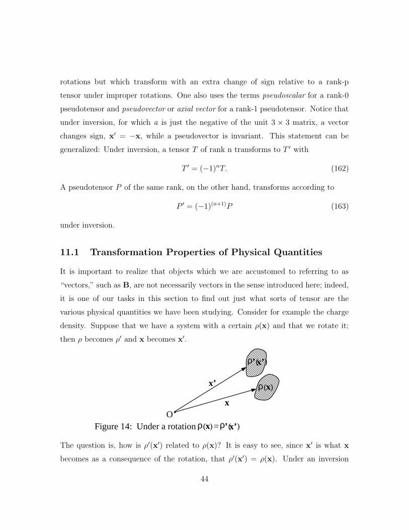
density. Suppose that we have a system with a certain ρ(x) and that we rotate it;

then ρ becomes ρ′ and x becomes x′.

ρ( )x

x

x’

ρ ( )x’’

OFigure 14: Under a rotation ρ( )x ρ ( )x’’=

The question is, how is ρ′(x′) related to ρ(x)? It is easy to see, since x′ is what x

becomes as a consequence of the rotation, that ρ′(x′) = ρ(x). Under an inversion

44

also, this relation is true. Hence we conclude that the charge density is a scalar or

rank-0 tensor.

An example of a vector or rank-1 tensor is, of course, x. Similarly, from this fact

one may show that the operator ∇ is a rank-1 tensor (Differential operators can also

be tensors or components of tensors);

∂

∂x′i=∑

j

aij∂

∂xj. (164)

What then is ∇ρ? From the (known) transformation properties of ρ and of ∇, it

is easy to show that it is a rank-1 tensor. The gradient of any scalar function is a

rank-1 tensor. Similarly, one may show that the inner product of two rank-1 tensors,

or vectors, is a scalar as is the inner product of two rank-1 pseudotensors; the inner

product of a rank-1 tensor and a rank-1 pseudotensor is a pseudoscalar; and the

gradient of a pseudoscalar is a rank-1 pseudotensor.

All of the foregoing are quite easy to demonstrate. A little harder is the crossprod-

uct of two vectors (rank-1 tensors). Consider that b and c are rank-1 tensors. Their

cross product may be written as

u = b× c (165)

with a Cartesian component given by

ui =∑

j,k

εijkbjck (166)

where

εijk ≡

+1 if (i, j, k) = (1, 2, 3), (2, 3, 1), (3, 1, 2)

−1 if (i, j, k) = (2, 1, 3), (1, 3, 2), (3, 2, 1)

0 otherwise.

(167)

If we define εijk to be given by this equation in all frames, then we can show that it

is a rank-3 pseudotensor. Alternatively, we can use Eq. (164) to specify it in a single

frame, define it to be a rank-3 pseudotensor, and then show that it is given by

Eq. (164) in any frame. However one chooses to do it, one can use this object, called

45

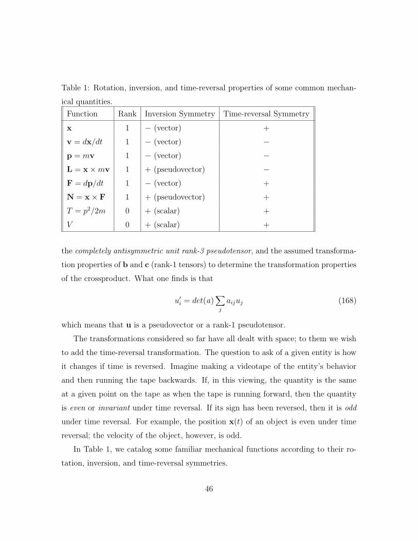
Table 1: Rotation, inversion, and time-reversal properties of some common mechan-

ical quantities.

Function Rank Inversion Symmetry Time-reversal Symmetry

x 1 − (vector) +

v = dx/dt 1 − (vector) −p = mv 1 − (vector) −L = x×mv 1 + (pseudovector) −F = dp/dt 1 − (vector) +

N = x× F 1 + (pseudovector) +

T = p2/2m 0 + (scalar) +

V 0 + (scalar) +

the completely antisymmetric unit rank-3 pseudotensor, and the assumed transforma-

tion properties of b and c (rank-1 tensors) to determine the transformation properties

of the crossproduct. What one finds is that

u′i = det(a)∑

j

aijuj (168)

which means that u is a pseudovector or a rank-1 pseudotensor.

The transformations considered so far have all dealt with space; to them we wish

to add the time-reversal transformation. The question to ask of a given entity is how

it changes if time is reversed. Imagine making a videotape of the entity’s behavior

and then running the tape backwards. If, in this viewing, the quantity is the same

at a given point on the tape as when the tape is running forward, then the quantity

is even or invariant under time reversal. If its sign has been reversed, then it is odd

under time reversal. For example, the position x(t) of an object is even under time

reversal; the velocity of the object, however, is odd.

In Table 1, we catalog some familiar mechanical functions according to their ro-

tation, inversion, and time-reversal symmetries.

46

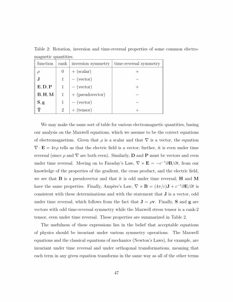
Table 2: Rotation, inversion and time-reversal properties of some common electro-

magnetic quantities.

function rank inversion symmetry time-reversal symmetry

ρ 0 + (scalar) +

J 1 − (vector) −E,D,P 1 − (vector) +

B,H,M 1 + (pseudovector) −S,g 1 − (vector) −T 2 + (tensor) +

We may make the same sort of table for various electromagnetic quantities, basing

our analysis on the Maxwell equations, which we assume to be the correct equations

of electromagnetism. Given that ρ is a scalar and that ∇ is a vector, the equation

∇ · E = 4πρ tells us that the electric field is a vector; further, it is even under time

reversal (since ρ and ∇ are both even). Similarly, D and P must be vectors and even

under time reversal. Moving on to Faraday’s Law, ∇ × E = −c−1∂B/∂t, from our

knowledge of the properties of the gradient, the cross product, and the electric field,

we see that B is a pseudovector and that it is odd under time reversal; H and M

have the same properties. Finally, Ampere’s Law, ∇ × B = (4π/c)J + c−1∂E/∂t is

consistent with these determinations and with the statement that J is a vector, odd

under time reversal, which follows from the fact that J = ρv. Finally, S and g are

vectors with odd time-reversal symmetry while the Maxwell stress tensor is a rank-2

tensor, even under time reversal. These properties are summarized in Table 2.

The usefulness of these expressions lies in the belief that acceptable equations

of physics should be invariant under various symmetry operations. The Maxwell

equations and the classical equations of mechanics (Newton’s Laws), for example, are

invariant under time reversal and under orthogonal transformations, meaning that

each term in any given equation transforms in the same way as all of the other terms

47

in that equation11. If we believe that this should be true of all elementary equations

of classical physics, then there are certain implied constraints on the form of the

equations. Consider as an example the relation between P and E. Supposing that

one can make an expansion of a component of P in terms of the components of E,

we have

Pi =∑

j

αijEj +∑

jk

βijkEjEk +∑

jkl

γijklEjEkEl + ... (169)

where, since P and E are both rank-1 tensors, invariant under time reversal, it follows,

using the invariance argument, that the coefficients αij are the components of a rank-

2 tensor, invariant under time reversal; the βijk are components of a rank-3 tensor,

invariant under time reversal; and the γijkl are components of a rank-4 tensor, also

invariant under time reversal.

If we now add some statement about the properties of the medium, we can get

further conditions. In the simplest case of an isotropic material, it must be the

case that each of these tensors is invariant under orthogonal transformations. This

condition severely limits their forms; in particular, it means that αij = αδij . We can

see this by appealing to the transformation properties of second rank tensors. Thus,

αij must transform like xixj, or

α′nm = aniamjαij (170)

Since the medium is isotropic, we require that α′ij = αij. The only way to satisfy

both of these conditions of transformation is if

α′nm = αaniami = αδnm (171)

The same type of thing cannot be done with β, so that βijk = 0, bu we can perform

similar manipulations on γ so the coefficients γijkl are such as to produce

∑

jkl

γijklEiEjEl = γ(E · E)E (172)

11Of course there are some equations, like Ohm’s Law, which describe truly irreversible processes

for which time reversal invariance does not hold.

48

where γ is a constant. Thus, through third-order terms, the expansion of P in terms

of E must have the form

P = αE + γE2E. (173)

The general forms of many other less obvious relations may be determined by similar

considerations.

12 Do Maxwell’s Equations Allow Magnetic Monopoles?

The answer is yes, but only in a restricted, and trivial, sense. If there were mag-

netic charges of density ρm and an associated magnetic current density Jm, with a

corresponding conservation law

∂ρm∂t

+∇ · Jm = 0, (174)

then the field equations would read

∇ ·B = 4πρm ∇×H =4π

cJ +

1

c

∂D

∂t

∇ ·D = 4πρ ∇× E = −4π

cJm −

1

c

∂B

∂t. (175)

In fact, the Maxwell equations as we understand them can be put into this form by

making a particular kind of transformation, called a duality transformation of the

fields and sources. Introduce

E = E′ cos η + H′ sin η D = D′ cos η + B′ sin η

H = −E′ sin η + H′ cos η B = −D′ sin η + B′ cos η

ρ = ρ′ cos η + ρ′m sin η J = J′ cos η + J′m sin η

ρm = −ρ′ sin η + ρ′m cos η Jm = −J′ sin η + J′m cos η. (176)

where η is an arbitrary real constant.

If one now substitutes these into the generalized field equations, one finds, upon

separating the coefficients of sin η from those of cos η (These must be independent

49

because η is arbitrary), that the primed fields and sources obey an identical set of

field equations. What this means is that the Maxwell equations (with no magnetic

sources) may be thought of as a special case of the generalized field equations, one

in which η is chosen so that ρm and Jm are equal to zero. From the form of the

transformations for the sources, we see that this is possible if the ratio of ρ to ρm for

each source (particle)is the same as that for all of the other sources (particles). Hence

it is meaningless to say that there are no magnetic monopoles; the real question is

whether all elementary particles have the same ratio of electric to magnetic charge.

If they do, then Maxwell’s equations are correct and correspond, as stated above, to

a particular choice of η in the more general field equations.

If one subjects the electron and proton to scrutiny regarding the question of

whether they have the same ratio of electric to magnetic charge, one finds that if

one defines (by choice of η) the magnetic charge of the electron to be zero, then

experimentally the magnetic charge of the proton is known to be smaller than 10−24

of its electric charge. That’s pretty good evidence for its being zero.

But there remains the question whether there are other kinds of particles, not

yet discovered, which have a different ratio ρ/ρm than do electrons and protons.

Dirac, for example, has given a simple and clever argument which shows that the

quantization of the electric charge follows from the mere existence of an electrically

uncharged magnetic monopole. Moreover, the argument gives the magnetic charge g

of the monopole as g = nhc/4πe where n is any integer and h is Planck’s constant.

This is, in comparison with the electric charge, very large so that it ought to be in

principle easy to detect a “Dirac monopole” should there by any of them around. So

far, none has been reliably detected.

50

A Helmholtz’ Theorem

Any vector function of position C(x) can be written as the sum of two vector functions

such that the divergence vanishes for one and the curl vanishes for the other. In other

words, the decomposition

C(x) = D(x) + F(x) (177)

is always possible, where

∇ ·D = 0 ∇× F = 0 (178)

Proof. We may satisfy the two conditions for F and D, by writing

D = ∇×A F = −∇Φ . (179)

Then taking the curl and divergence of these equations respectively, we can write

∇2Φ = −∇ ·C ∇× (∇×A) = ∇×C . (180)

We already know how to solve these solutions (at least in Cartesian coordinates).

Φ(x′) =1

4π

∫

Vd3x∇ ·C(x)

|x− x′| A(x′) =1

4π

∫

Vd3x∇×C(x)

|x− x′| (181)

Since D and F can now be found from these potentials, we have demonstrated the

decomposition claimed by Helmholtz’ Theorem, and thus proved it.

An interesting corollary of this theorem is that a vector function is completely

determined if its curl and divergence are known everywhere. The field F = −∇Φ,

where produced by a point source, is longitudinal to the vector from the source to the

point where the field is evaluated. The field D = ∇×A is transverse to the vector

from the source to the field point. Thus F is typically called the longitudinal, and D

the transverse, part of C.

51