MaxEnt: Training, Smoothing, Tagging Advanced Statistical Methods in NLP Ling572 February 7, 2012 1.
104
MaxEnt: Training, Smoothing, Tagging Advanced Statistical Methods in NLP Ling572 February 7, 2012 1
-
Upload
margaret-george -
Category
Documents
-
view
218 -
download
0
Transcript of MaxEnt: Training, Smoothing, Tagging Advanced Statistical Methods in NLP Ling572 February 7, 2012 1.
1
MaxEnt: Training, Smoothing, Tagging
Advanced Statistical Methods in NLPLing572
February 7, 2012
2
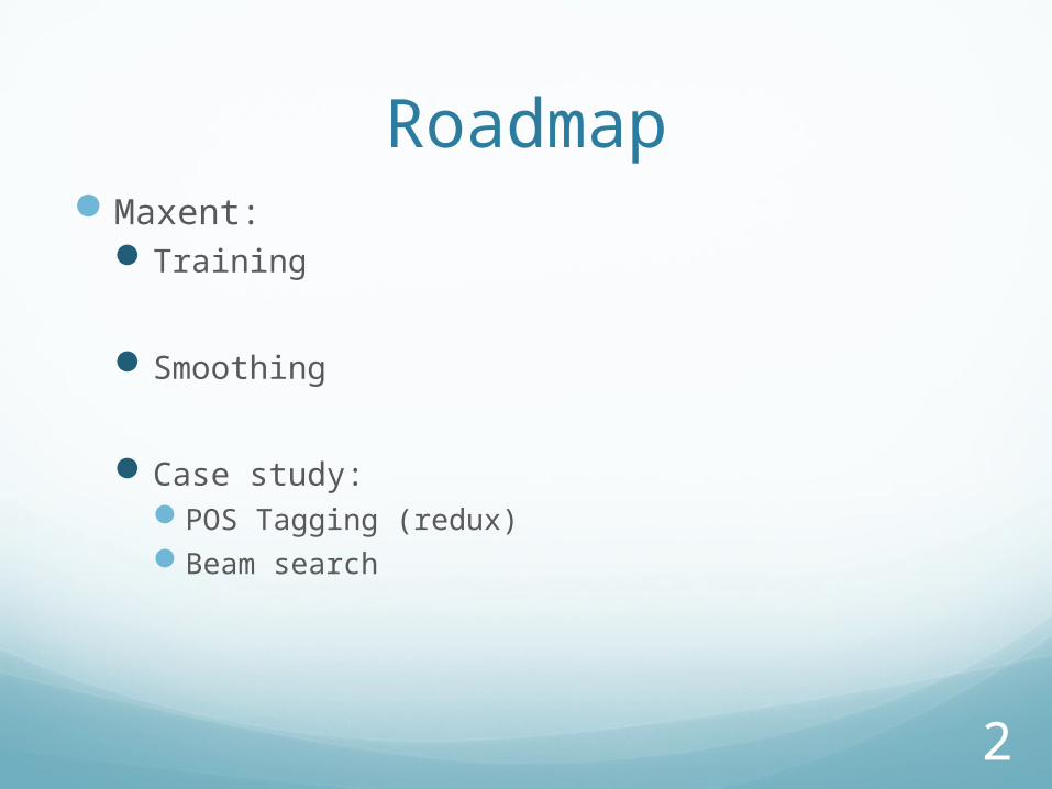
RoadmapMaxent:
Training
Smoothing
Case study: POS Tagging (redux)Beam search

3
Training

4
TrainingLearn λs from training data
5
TrainingLearn λs from training data
Challenge: Usually can’t solve analyticallyEmploy numerical methods
6
TrainingLearn λs from training data
Challenge: Usually can’t solve analyticallyEmploy numerical methods
Main different techniques:Generalized Iterative Scaling (GIS, Darroch &Ratcliffe,
‘72)
Improved Iterative Scaling (IIS, Della Pietra et al, ‘95)
L-BFGS,…..
7
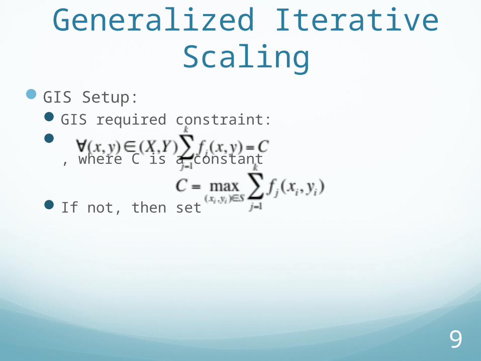
Generalized Iterative Scaling
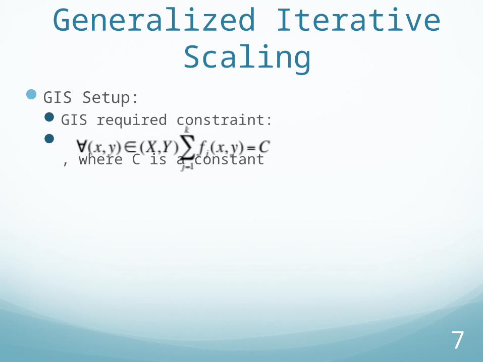
GIS Setup:GIS required constraint: , where C is a constant
8
Generalized Iterative Scaling
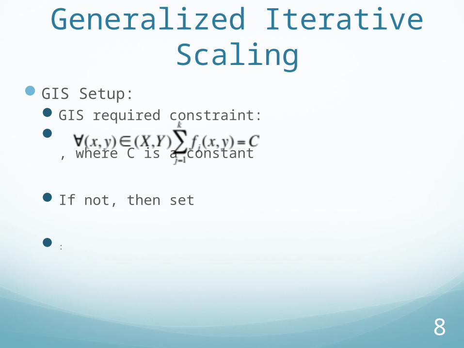
GIS Setup:GIS required constraint: , where C is a constant
If not, then set
:
9
Generalized Iterative Scaling
GIS Setup:GIS required constraint: , where C is a constant
If not, then set
10
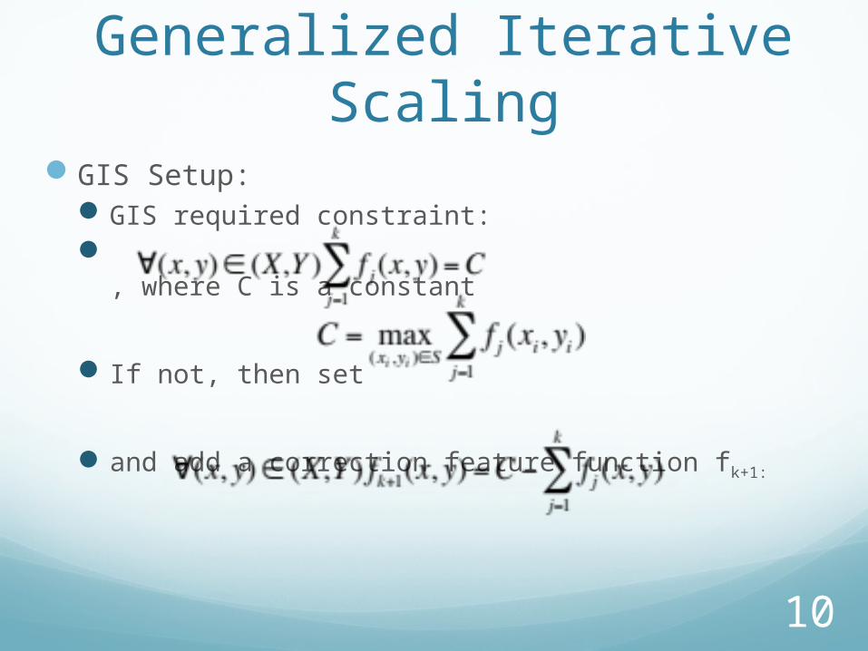
Generalized Iterative Scaling
GIS Setup:GIS required constraint: , where C is a constant
If not, then set
and add a correction feature function fk+1:
11
Generalized Iterative Scaling
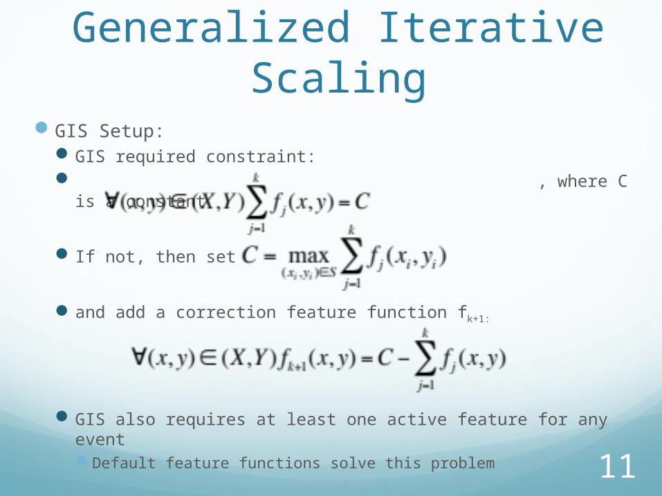
GIS Setup:GIS required constraint: , where C is a constant
If not, then set
and add a correction feature function fk+1:
GIS also requires at least one active feature for any eventDefault feature functions solve this problem
12
GIS IterationCompute the empirical expectation
13
GIS IterationCompute the empirical expectation
Initialization:λj(0) ; set to 0 or some value
14
GIS IterationCompute the empirical expectation
Initialization:λj(0) ; set to 0 or some value
Iterate until convergence for each j:
15
GIS IterationCompute the empirical expectation
Initialization:λj(0) ; set to 0 or some value
Iterate until convergence for each j:Compute p(y|x) under the current model
16
GIS IterationCompute the empirical expectation
Initialization:λj(0) ; set to 0 or some value
Iterate until convergence for each j:Compute p(y|x) under the current model
Compute model expectation under current model
17
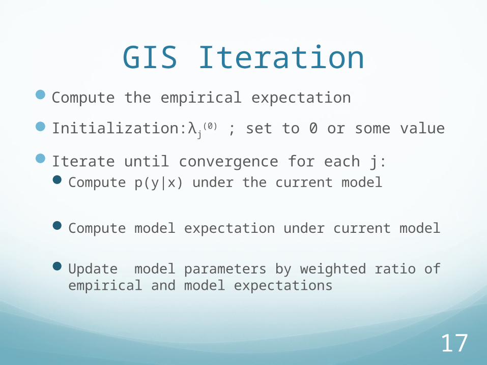
GIS IterationCompute the empirical expectation
Initialization:λj(0) ; set to 0 or some value
Iterate until convergence for each j:Compute p(y|x) under the current model
Compute model expectation under current model
Update model parameters by weighted ratio of empirical and model expectations
18
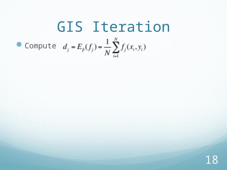
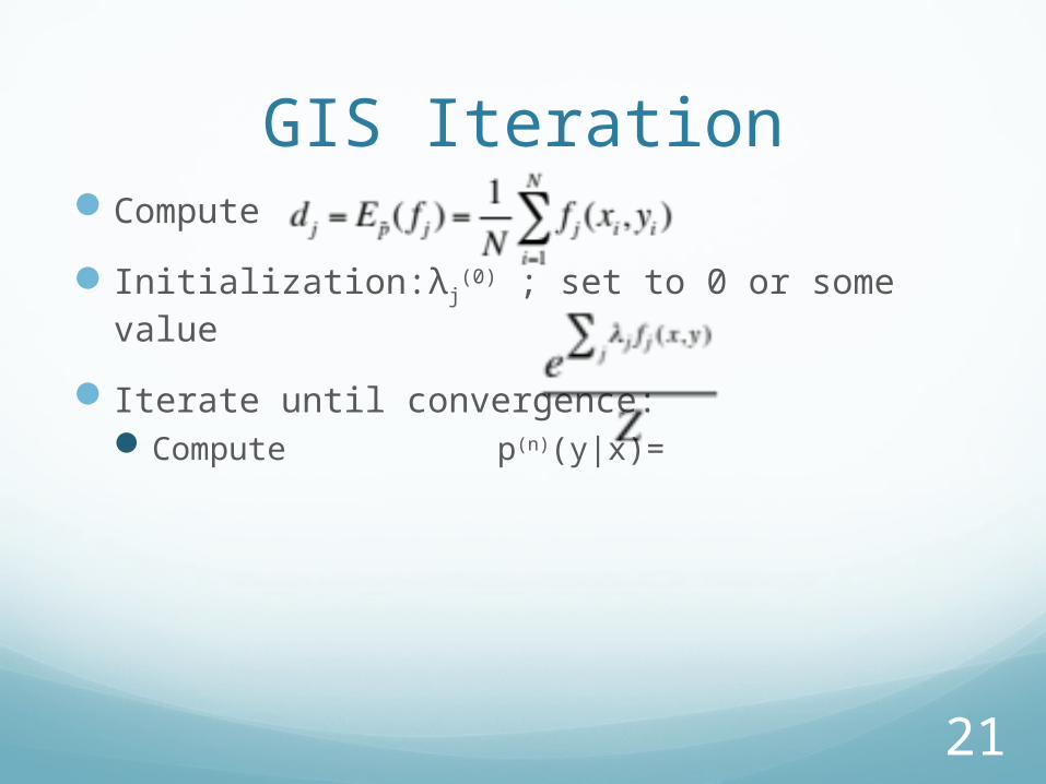
GIS IterationCompute
19
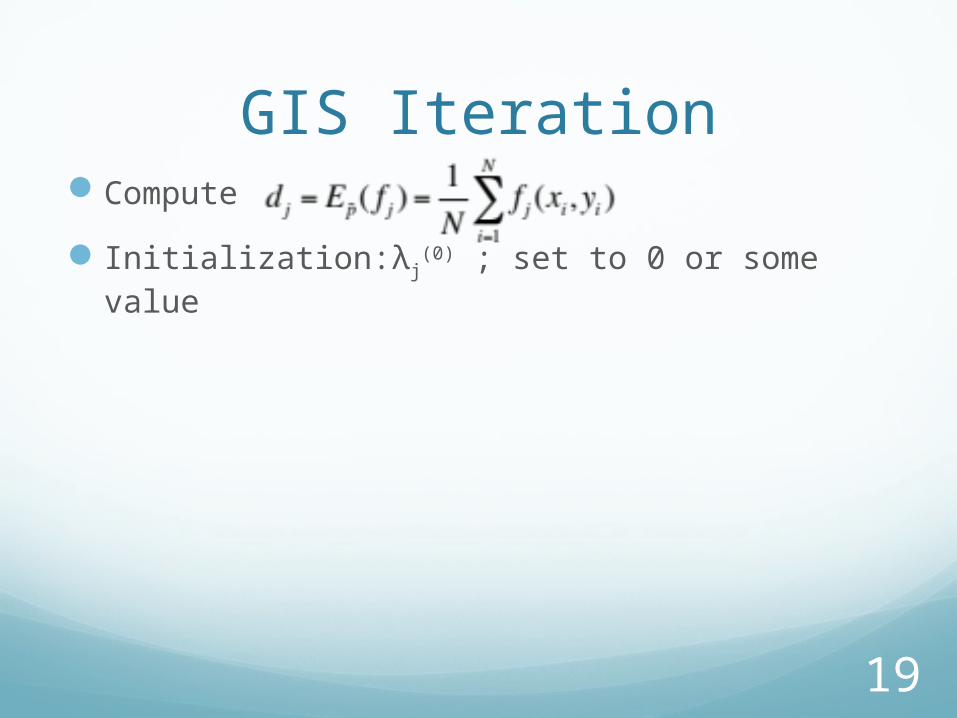
GIS IterationCompute
Initialization:λj(0) ; set to 0 or some value
20
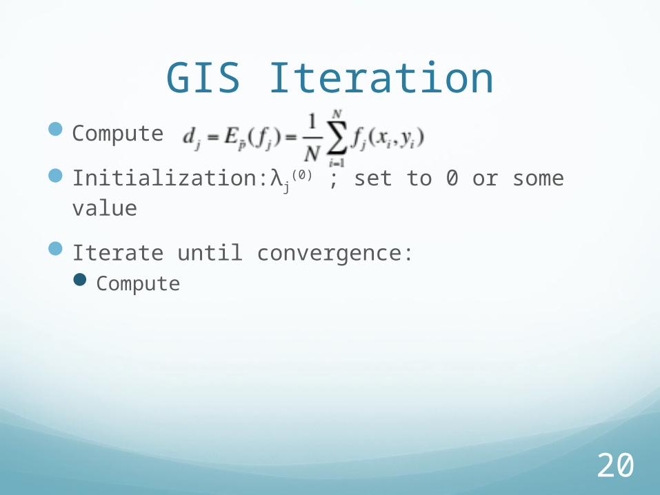
GIS IterationCompute
Initialization:λj(0) ; set to 0 or some value
Iterate until convergence:Compute
21
GIS IterationCompute
Initialization:λj(0) ; set to 0 or some value
Iterate until convergence:Compute p(n)(y|x)=
22
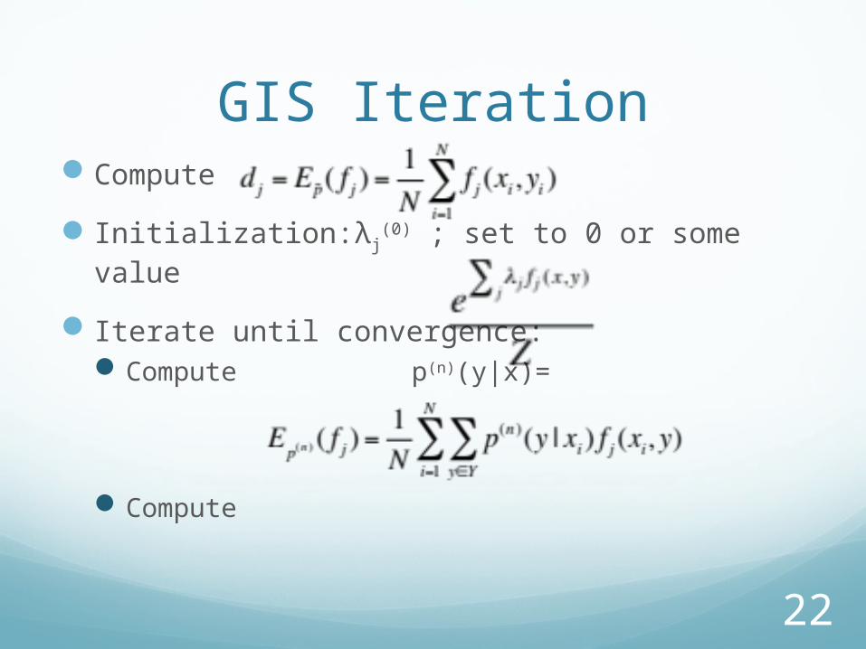
GIS IterationCompute
Initialization:λj(0) ; set to 0 or some value
Iterate until convergence:Compute p(n)(y|x)=
Compute
23
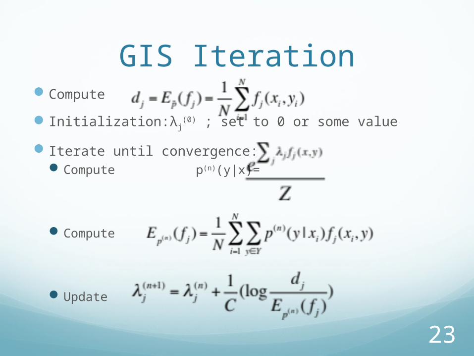
GIS IterationCompute
Initialization:λj(0) ; set to 0 or some value
Iterate until convergence:Compute p(n)(y|x)=
Compute
Update

24
ConvergenceMethods have convergence guarantees
25
ConvergenceMethods have convergence guarantees
However, full convergence may take very long time
26
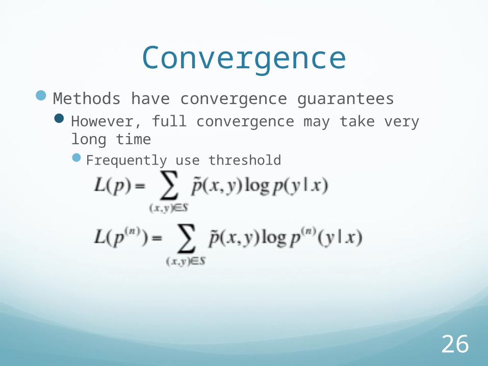
ConvergenceMethods have convergence guarantees
However, full convergence may take very long timeFrequently use threshold
27
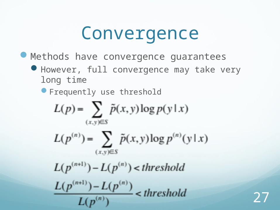
ConvergenceMethods have convergence guarantees
However, full convergence may take very long timeFrequently use threshold
28
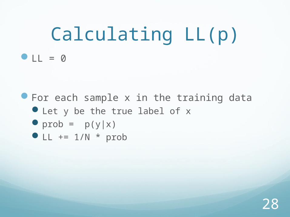
Calculating LL(p)LL = 0
For each sample x in the training dataLet y be the true label of xprob = p(y|x)LL += 1/N * prob

29
Running TimeFor each iteration the running time is:
30
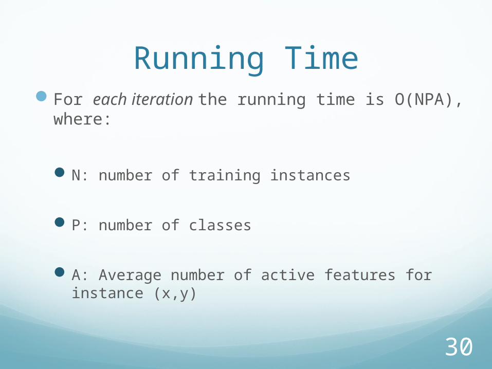
Running TimeFor each iteration the running time is O(NPA),
where:
N: number of training instances
P: number of classes
A: Average number of active features for instance (x,y)

31
L-BFGSLimited-memory version of
Broyden–Fletcher–Goldfarb–Shanno (BFGS) method
32
L-BFGSLimited-memory version of
Broyden–Fletcher–Goldfarb–Shanno (BFGS) method
Quasi-Newton method for unconstrained optimization
33
L-BFGSLimited-memory version of
Broyden–Fletcher–Goldfarb–Shanno (BFGS) method
Quasi-Newton method for unconstrained optimization
Good for optimization problems with many variables
34
L-BFGSLimited-memory version of
Broyden–Fletcher–Goldfarb–Shanno (BFGS) method
Quasi-Newton method for unconstrained optimization
Good for optimization problems with many variables
“Algorithm of choice” for MaxEnt and related models
35
L-BFGSReferences:
Nocedal, J. (1980). "Updating Quasi-Newton Matrices with Limited Storage". Mathematics of Computation 35: 773–782
Liu, D. C.; Nocedal, J. (1989)"On the Limited Memory Method for Large Scale Optimization". Mathematical Programming B 45 (3): 503–528
36
L-BFGSReferences:
Nocedal, J. (1980). "Updating Quasi-Newton Matrices with Limited Storage". Mathematics of Computation 35: 773–782
Liu, D. C.; Nocedal, J. (1989)"On the Limited Memory Method for Large Scale Optimization". Mathematical Programming B 45 (3): 503–528
Implementations: Java, Matlab, Python via scipy, R, etcSee Wikipedia page
37
SmoothingBased on Klein & Manning, 2003; F. Xia
38
SmoothingProblems of scale:
39
SmoothingProblems of scale:
Large numbers of featuresSome NLP problems in MaxEnt 1M features
Storage can be a problem
40
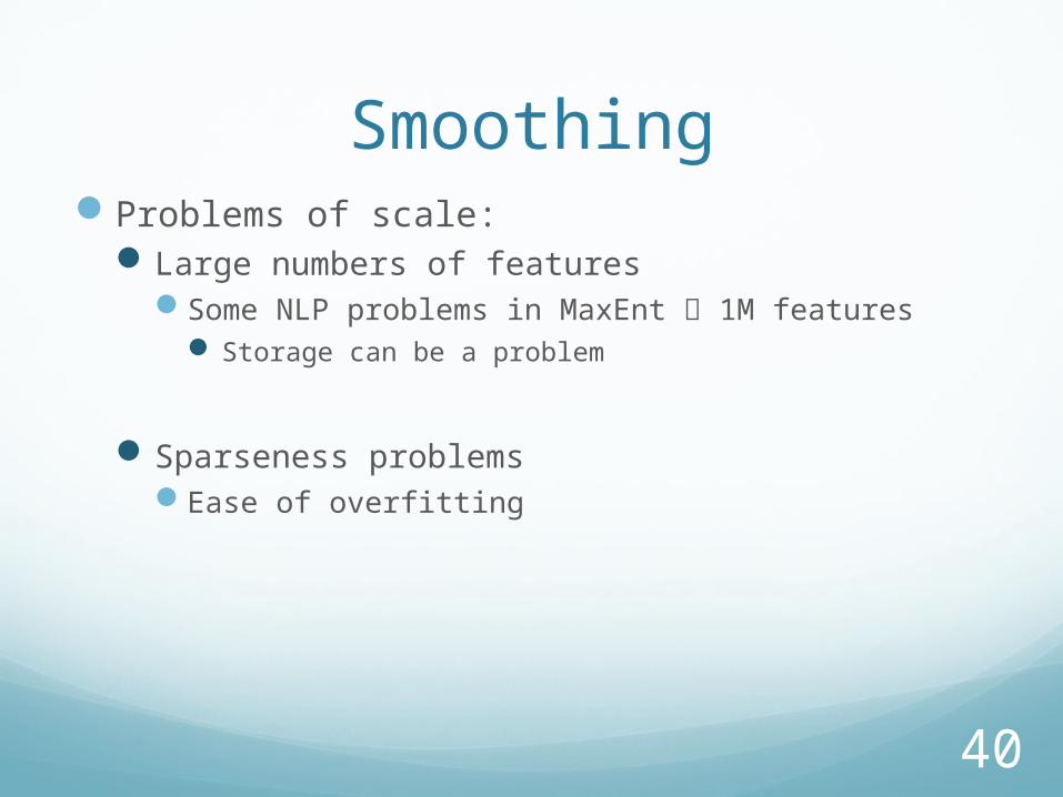
SmoothingProblems of scale:
Large numbers of featuresSome NLP problems in MaxEnt 1M features
Storage can be a problem
Sparseness problemsEase of overfitting
41
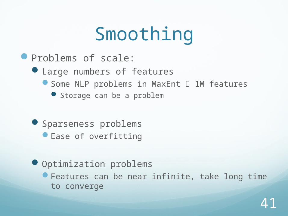
SmoothingProblems of scale:
Large numbers of featuresSome NLP problems in MaxEnt 1M features
Storage can be a problem
Sparseness problemsEase of overfitting
Optimization problemsFeatures can be near infinite, take long time to
converge
42
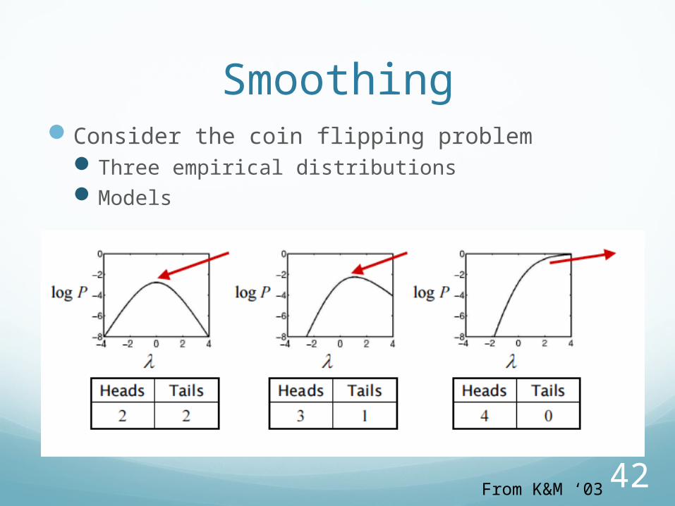
SmoothingConsider the coin flipping problem
Three empirical distributionsModels
From K&M ‘03
43
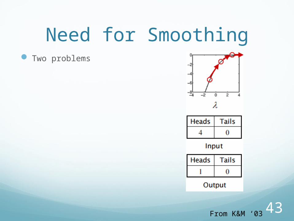
Need for Smoothing Two problems
From K&M ‘03
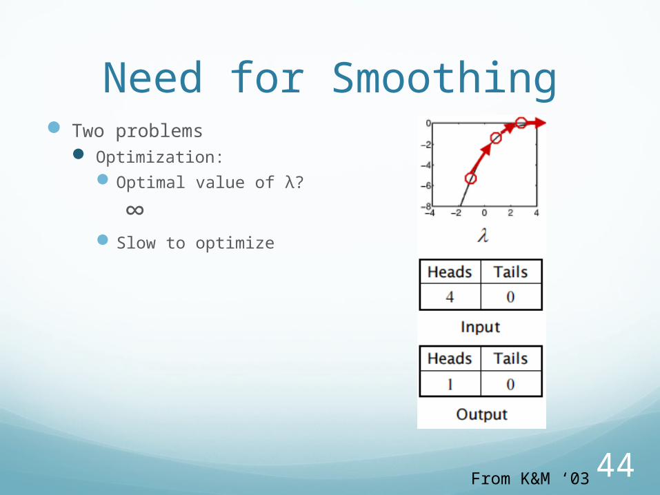
44
Need for Smoothing Two problems
Optimization:Optimal value of λ?
∞Slow to optimize
From K&M ‘03
45
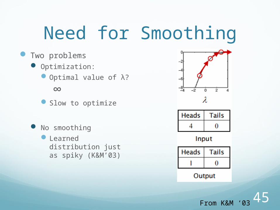
Need for Smoothing Two problems
Optimization:Optimal value of λ?
∞Slow to optimize
No smoothingLearned distribution
just as spiky (K&M’03)
From K&M ‘03

46
Possible Solutions
47
Possible SolutionsEarly stopping
Feature selection
Regularization

48
Early StoppingPrior use of early stopping
49
Early StoppingPrior use of early stopping
Decision tree heuristics
50
Early StoppingPrior use of early stopping
Decision tree heuristics
Similarly hereStop training after a few iterations
λwill have increased
Guarantees bounded, finite training time

51
Feature SelectionApproaches:
52
Feature SelectionApproaches:
Heuristic: Drop features based on fixed thresholdsi.e. number of occurrences
53
Feature SelectionApproaches:
Heuristic: Drop features based on fixed thresholdsi.e. number of occurrences
Wrapper methods:Add feature selection to training loop
54
Feature SelectionApproaches:
Heuristic: Drop features based on fixed thresholdsi.e. number of occurrences
Wrapper methods:Add feature selection to training loop
Heuristic approaches: Simple, reduce features, but could harm
performance
55
RegularizationIn statistics and machine learning, regularization
is any method of preventing overfitting of data by a model.
From K&M ’03, F. Xia
56
RegularizationIn statistics and machine learning, regularization
is any method of preventing overfitting of data by a model.
Typical examples of regularization in statistical machine learning include ridge regression, lasso, and L2-normin support vector machines.
From K&M ’03, F. Xia
57
RegularizationIn statistics and machine learning, regularization
is any method of preventing overfitting of data by a model.
Typical examples of regularization in statistical machine learning include ridge regression, lasso, and L2-normin support vector machines.
In this case, we change the objective function: log P(Y,λ|X) = log P(λ)+log P(Y|X,λ)
From K&M ’03, F. Xia
58
Prior Possible prior distributions: uniform, exponential
59
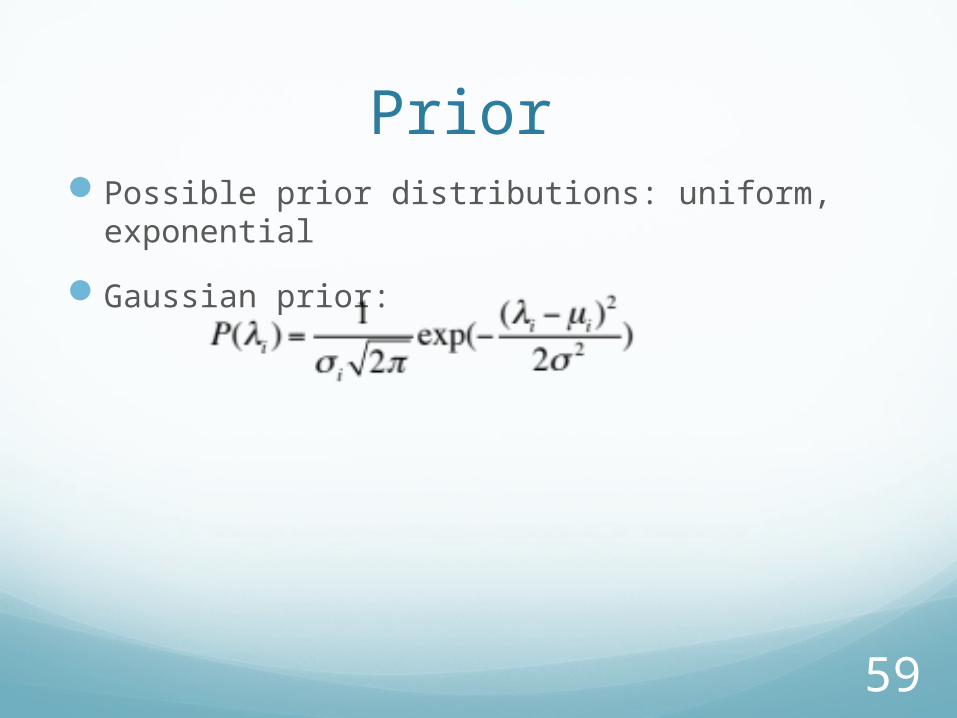
Prior Possible prior distributions: uniform, exponential
Gaussian prior:
60
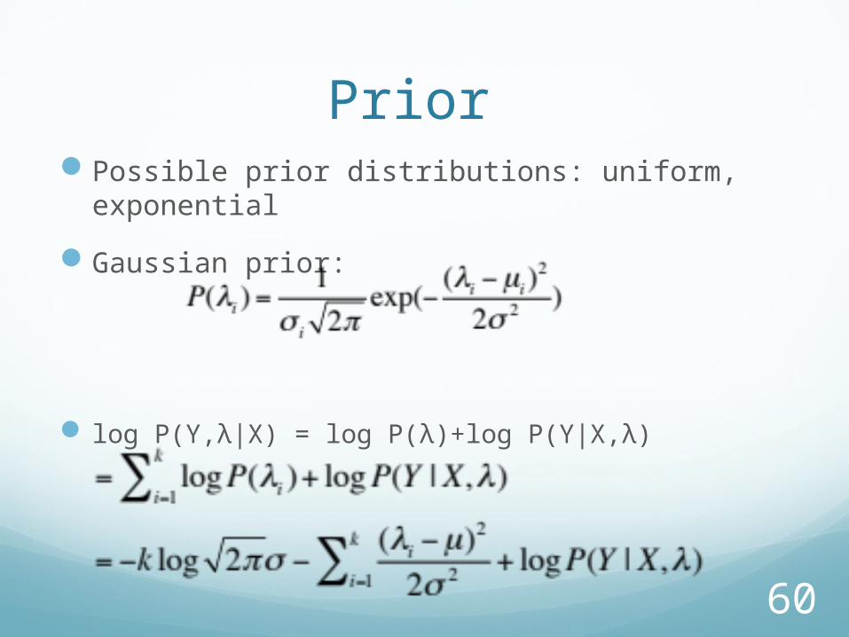
Prior Possible prior distributions: uniform, exponential
Gaussian prior:
log P(Y,λ|X) = log P(λ)+log P(Y|X,λ)
61
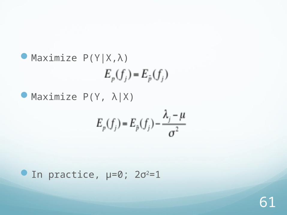
Maximize P(Y|X,λ)
Maximize P(Y, λ|X)
In practice, μ=0; 2σ2=1
62
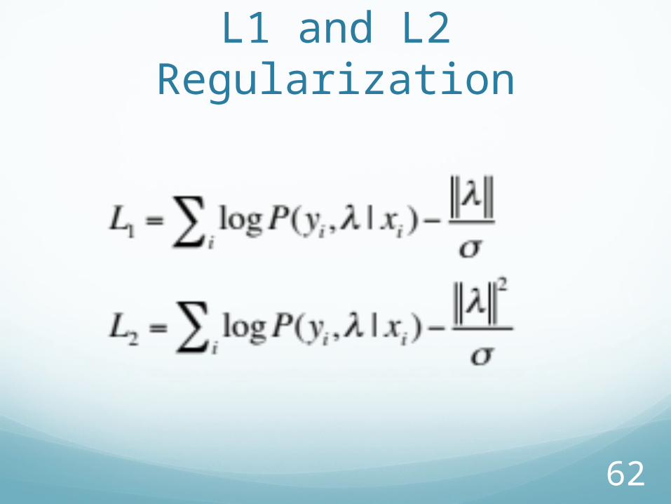
L1 and L2 Regularization
63
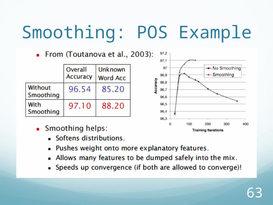
Smoothing: POS Example
64
Advantages of SmoothingSmooths distributions
65
Advantages of SmoothingSmooths distributions
Moves weight onto more informative features
66
Advantages of SmoothingSmooths distributions
Moves weight onto more informative features
Enables effective use of larger numbers of features
67
Advantages of SmoothingSmooths distributions
Moves weight onto more informative features
Enables effective use of larger numbers of features
Can speed up convergence
68
Summary: TrainingMany training methods:
Generalized Iterative Scaling (GIS)
Smoothing:Early stopping, feature selection, regularization
Regularization:Change objective function – add priorCommon prior: Gaussian priorMaximizing posterior not equivalent to max ent
69
MaxEnt POS Tagging
70
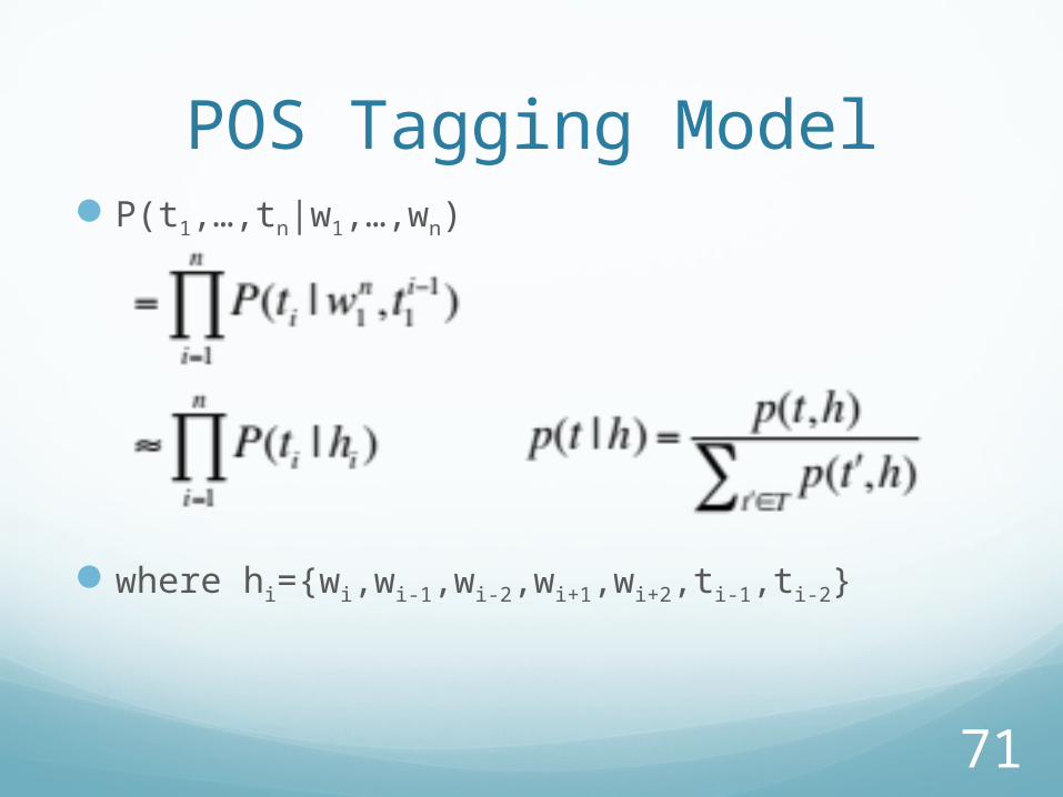
Notation(Ratnaparkhi, 1996)
h: history xWord and tag history
t: tag y
71
POS Tagging ModelP(t1,…,tn|w1,…,wn)
where hi={wi,wi-1,wi-2,wi+1,wi+2,ti-1,ti-2}
72
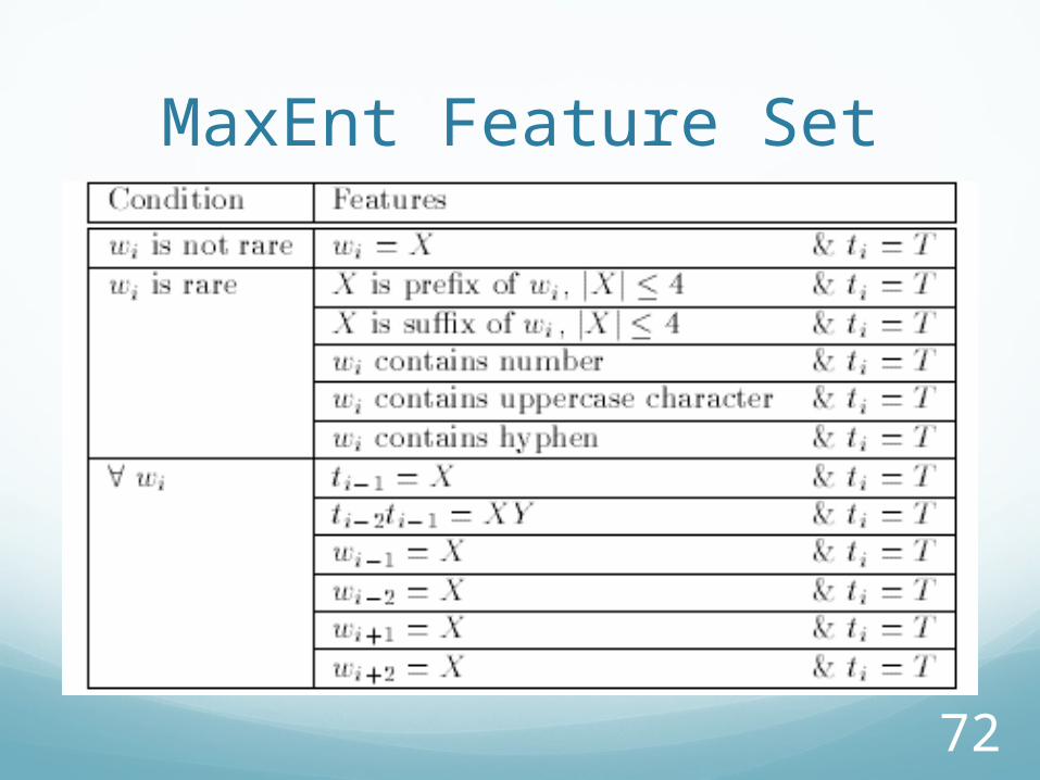
MaxEnt Feature Set
73
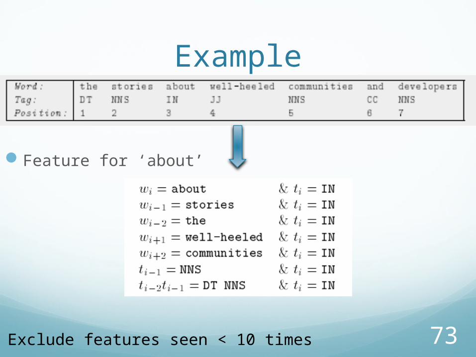
Example
Feature for ‘about’
Exclude features seen < 10 times

74
TrainingGIS
Training time: O(NTA)N: training set sizeT: number of tagsA: average number of features active for event
(h,t)
24 hours on a ‘96 machine
75
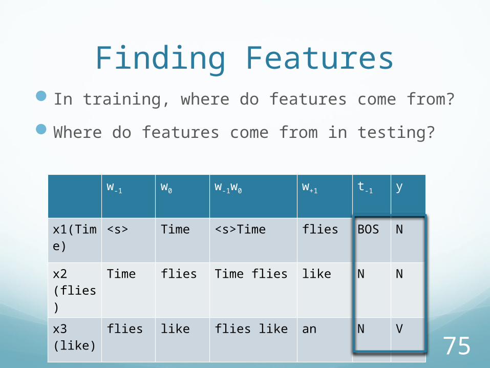
Finding FeaturesIn training, where do features come from?
Where do features come from in testing?
w-1 w0 w-1w0 w+1 t-1 y
x1(Time)
<s> Time <s>Time flies BOS N
x2 (flies)
Time flies Time flies like N N
x3 (like)
flies like flies like an N V
76
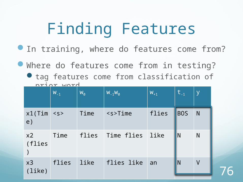
Finding FeaturesIn training, where do features come from?
Where do features come from in testing?tag features come from classification of prior word
w-1 w0 w-1w0 w+1 t-1 y
x1(Time)
<s> Time <s>Time flies BOS N
x2 (flies)
Time flies Time flies like N N
x3 (like)
flies like flies like an N V
77
DecodingGoal: Identify highest probability tag sequence
78
DecodingGoal: Identify highest probability tag sequence
Issues:Features include tags from previous words
Not immediately available
79
DecodingGoal: Identify highest probability tag sequence
Issues:Features include tags from previous words
Not immediately available
Uses tag historyJust knowing highest probability preceding tag
insufficient
80
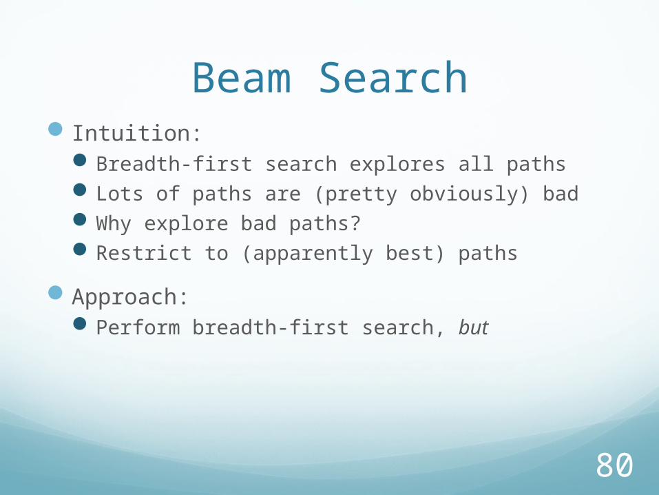
Beam SearchIntuition:
Breadth-first search explores all pathsLots of paths are (pretty obviously) badWhy explore bad paths?Restrict to (apparently best) paths
Approach:Perform breadth-first search, but
81
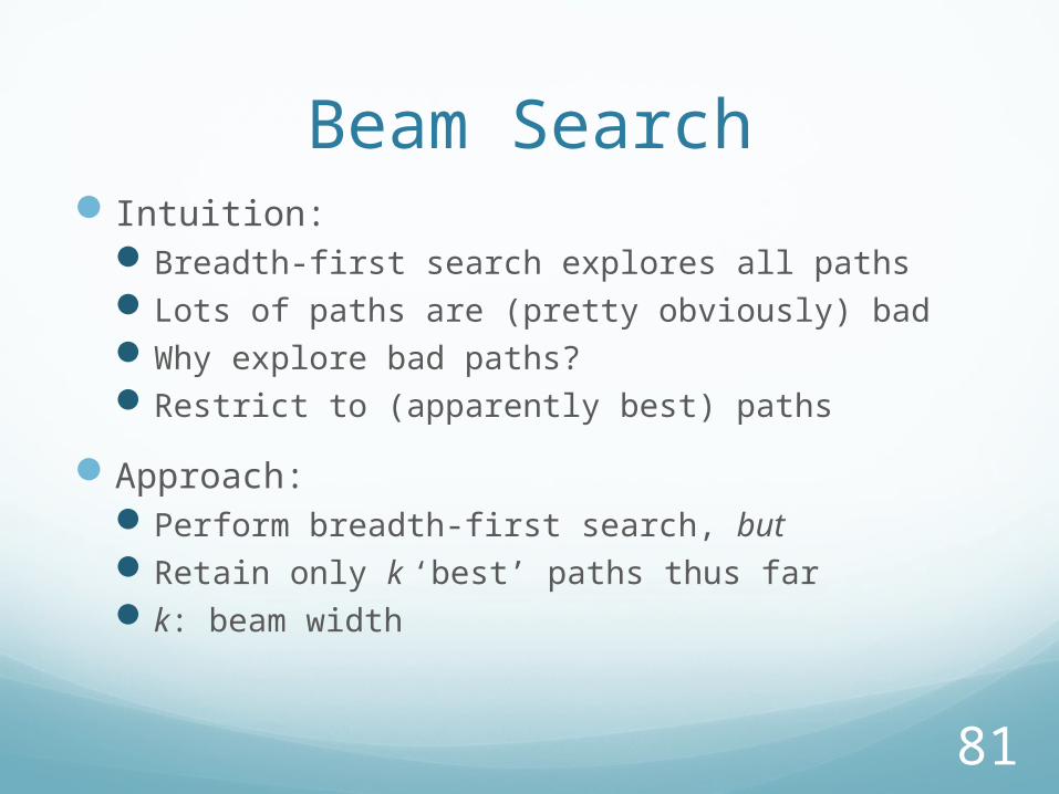
Beam SearchIntuition:
Breadth-first search explores all pathsLots of paths are (pretty obviously) badWhy explore bad paths?Restrict to (apparently best) paths
Approach:Perform breadth-first search, butRetain only k ‘best’ paths thus fark: beam width
82
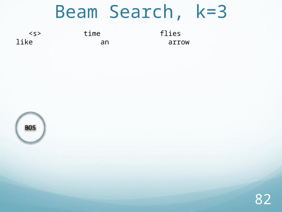
Beam Search, k=3 <s> time flies like an arrow
BOS
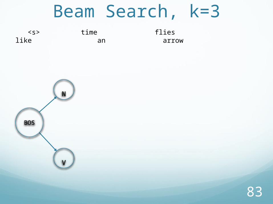
83
Beam Search, k=3
V
N
<s> time flies like an arrow
BOS
84
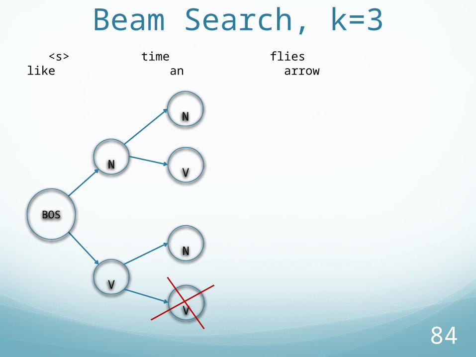
Beam Search, k=3
V
N
<s> time flies like an arrow
BOS
N
V
N
V
85
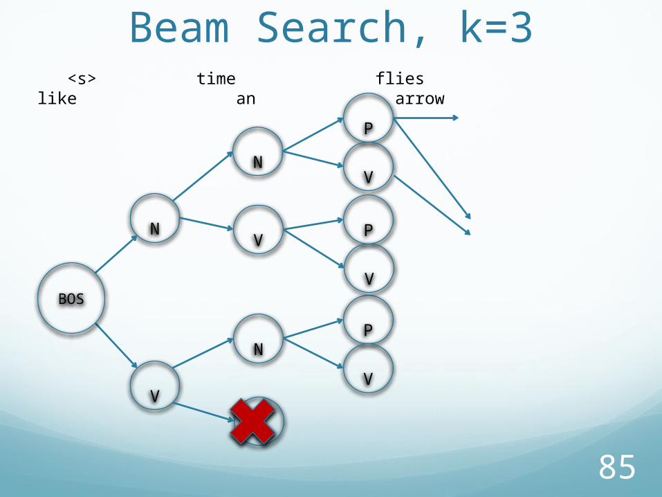
Beam Search, k=3
V
N
<s> time flies like an arrow
BOS
N
V
N
V
P
V
P
V
P
V
86
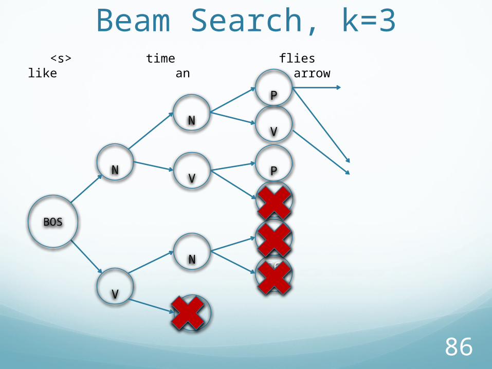
Beam Search, k=3
V
N
<s> time flies like an arrow
BOS
N
V
N
V
P
56V
P
V
P
V
87
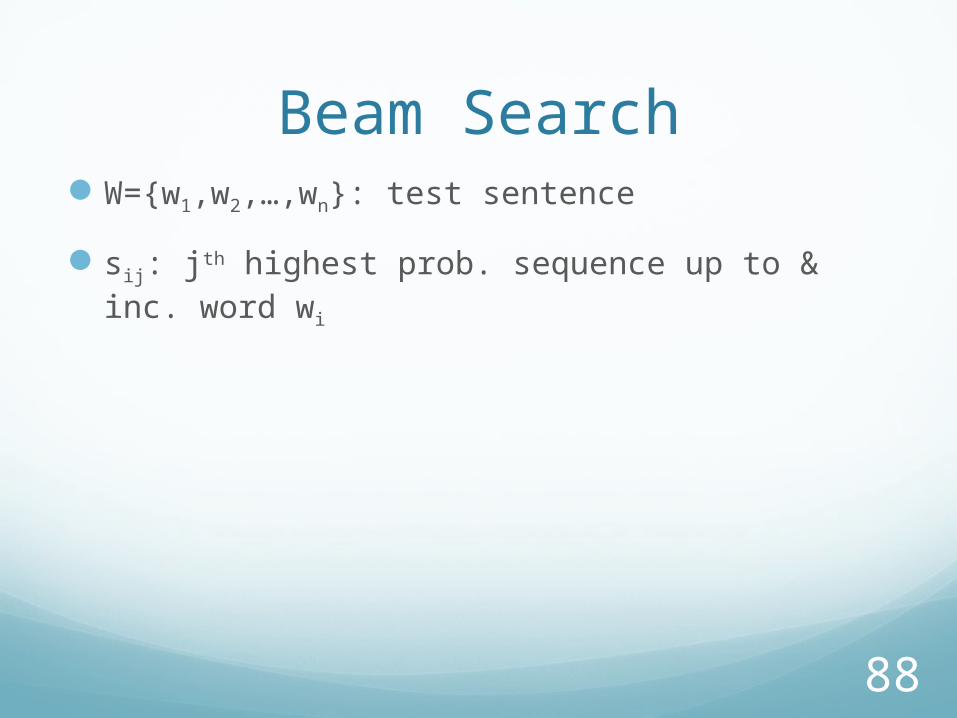
Beam SearchW={w1,w2,…,wn}: test sentence
88
Beam SearchW={w1,w2,…,wn}: test sentence
sij: jth highest prob. sequence up to & inc. word wi
89
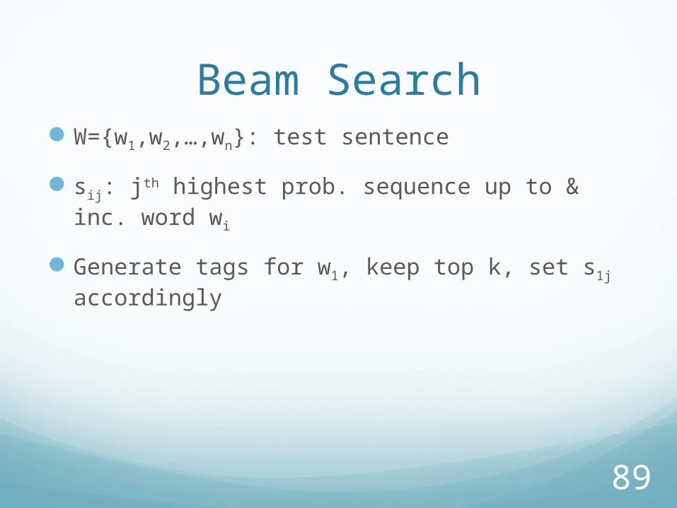
Beam SearchW={w1,w2,…,wn}: test sentence
sij: jth highest prob. sequence up to & inc. word wi
Generate tags for w1, keep top k, set s1j accordingly
90
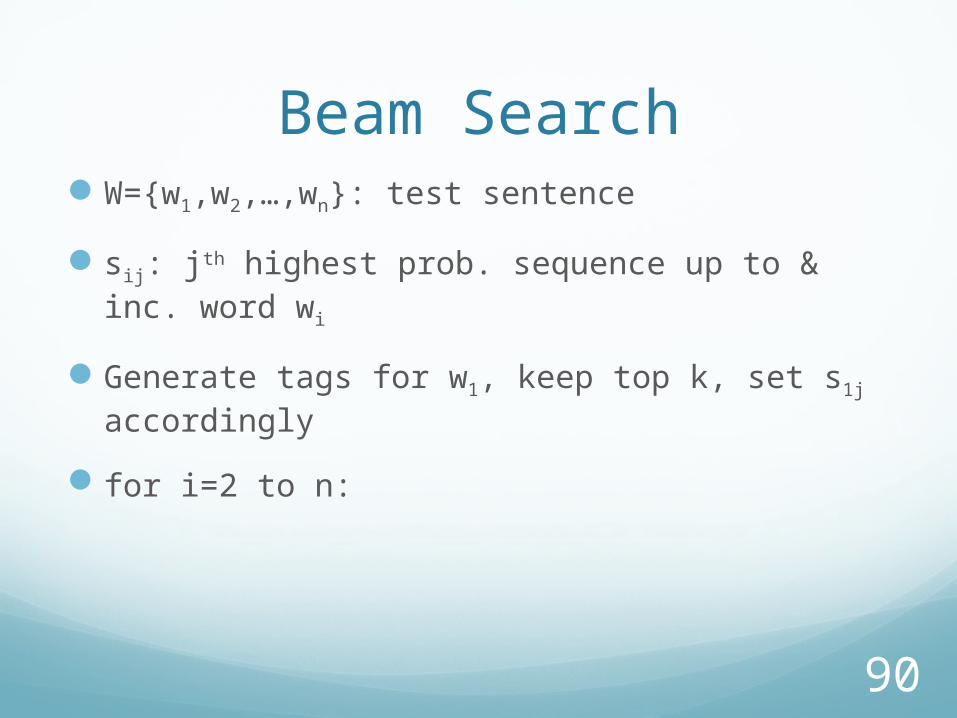
Beam SearchW={w1,w2,…,wn}: test sentence
sij: jth highest prob. sequence up to & inc. word wi
Generate tags for w1, keep top k, set s1j accordingly
for i=2 to n:
91
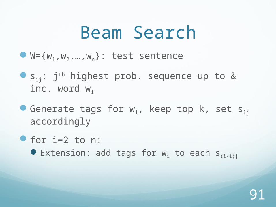
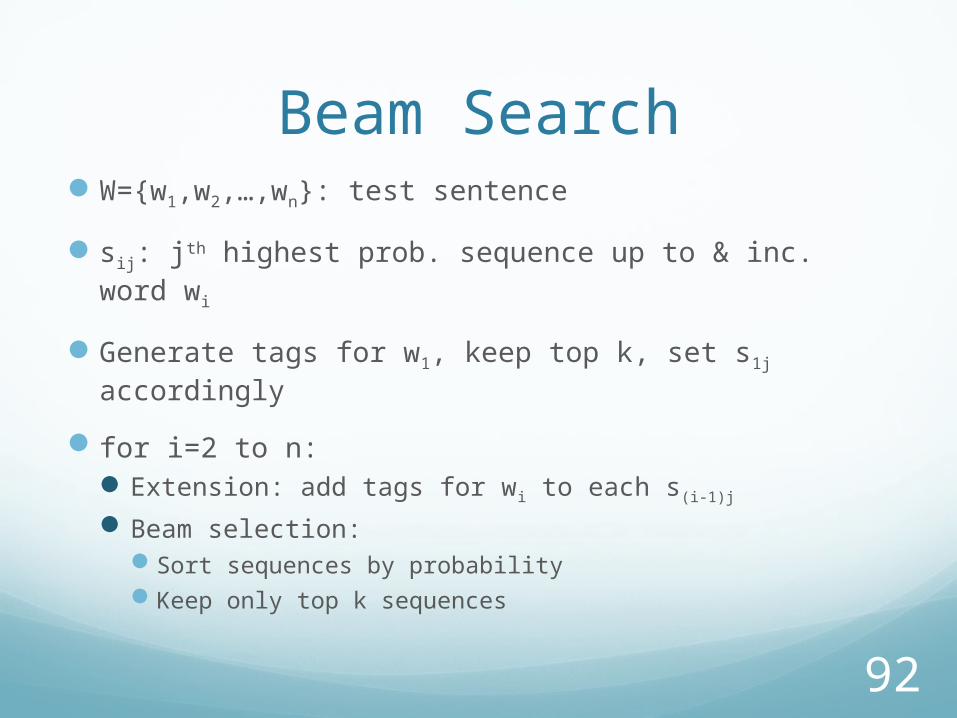
Beam SearchW={w1,w2,…,wn}: test sentence
sij: jth highest prob. sequence up to & inc. word wi
Generate tags for w1, keep top k, set s1j accordingly
for i=2 to n:Extension: add tags for wi to each s(i-1)j
92
Beam SearchW={w1,w2,…,wn}: test sentence
sij: jth highest prob. sequence up to & inc. word wi
Generate tags for w1, keep top k, set s1j accordingly
for i=2 to n:Extension: add tags for wi to each s(i-1)j
Beam selection: Sort sequences by probabilityKeep only top k sequences
93
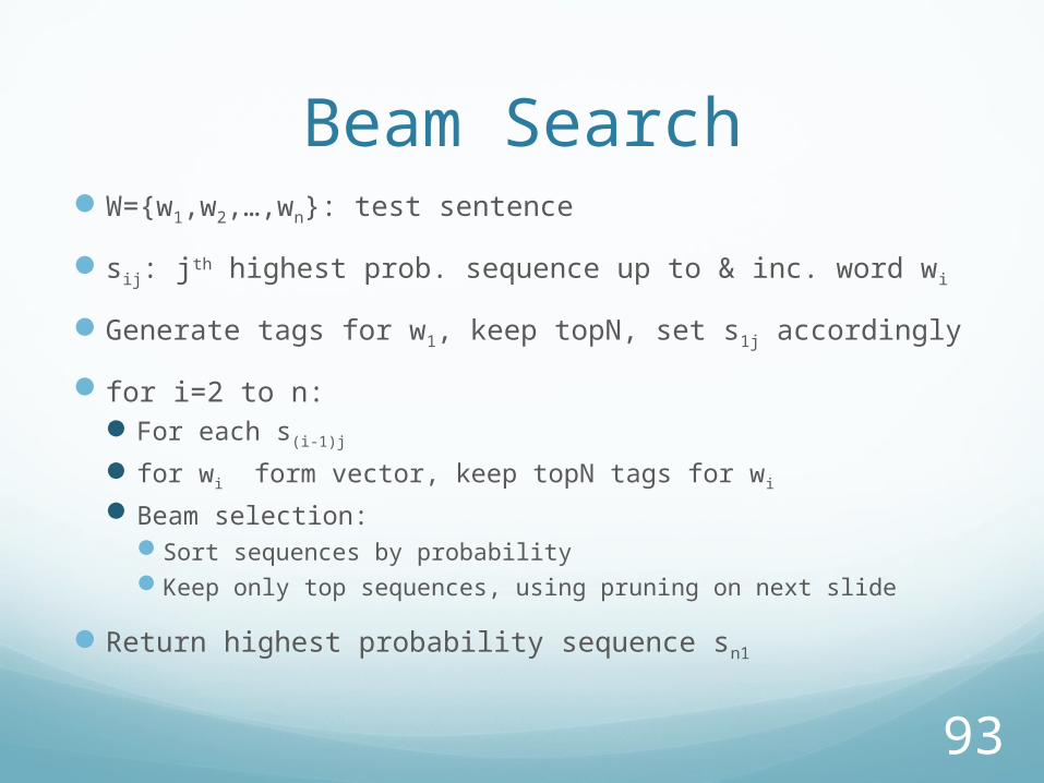
Beam SearchW={w1,w2,…,wn}: test sentence
sij: jth highest prob. sequence up to & inc. word wi
Generate tags for w1, keep topN, set s1j accordingly
for i=2 to n: For each s(i-1)j
for wi form vector, keep topN tags for wi
Beam selection: Sort sequences by probabilityKeep only top sequences, using pruning on next slide
Return highest probability sequence sn1
94
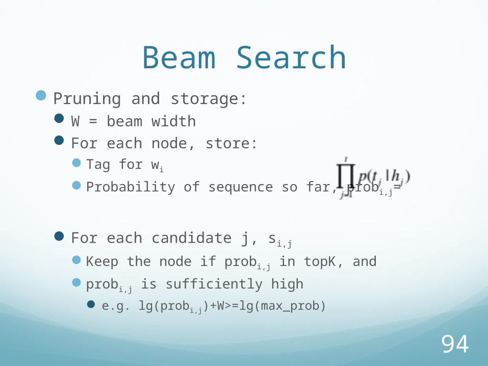
Beam SearchPruning and storage:
W = beam widthFor each node, store:
Tag for wi
Probability of sequence so far, probi,j=
For each candidate j, si,j
Keep the node if probi,j in topK, and
probi,j is sufficiently high
e.g. lg(probi,j)+W>=lg(max_prob)
95
DecodingTag dictionary:
known word: returns tags seen with word in training
unknown word: returns all tags
Beam width = 5
Running time: O(NTAB)N,T,A as beforeB: beam width
96
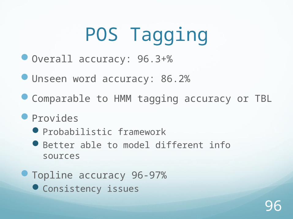
POS TaggingOverall accuracy: 96.3+%
Unseen word accuracy: 86.2%
Comparable to HMM tagging accuracy or TBL
ProvidesProbabilistic frameworkBetter able to model different info sources
Topline accuracy 96-97%Consistency issues
97
Beam SearchBeam search decoding:
Variant of breadth first searchAt each layer, keep only top k sequences
Advantages:
98
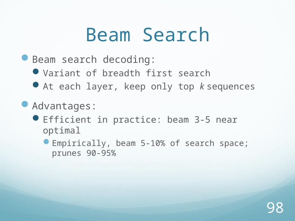
Beam SearchBeam search decoding:
Variant of breadth first searchAt each layer, keep only top k sequences
Advantages:Efficient in practice: beam 3-5 near optimal
Empirically, beam 5-10% of search space; prunes 90-95%
99
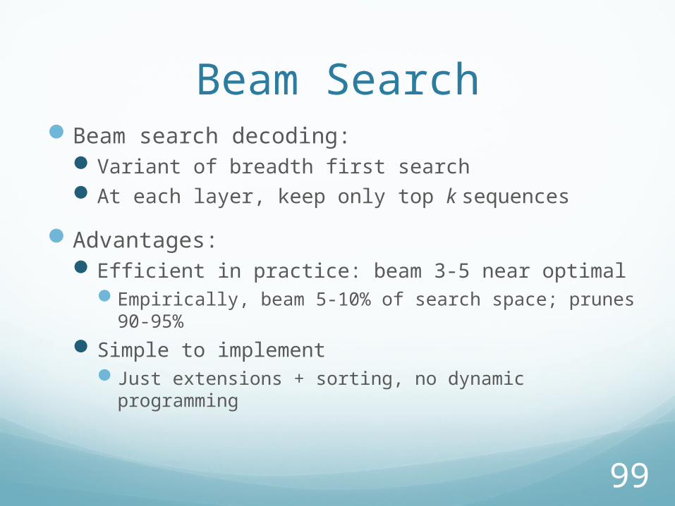
Beam SearchBeam search decoding:
Variant of breadth first searchAt each layer, keep only top k sequences
Advantages:Efficient in practice: beam 3-5 near optimal
Empirically, beam 5-10% of search space; prunes 90-95%
Simple to implementJust extensions + sorting, no dynamic programming
100
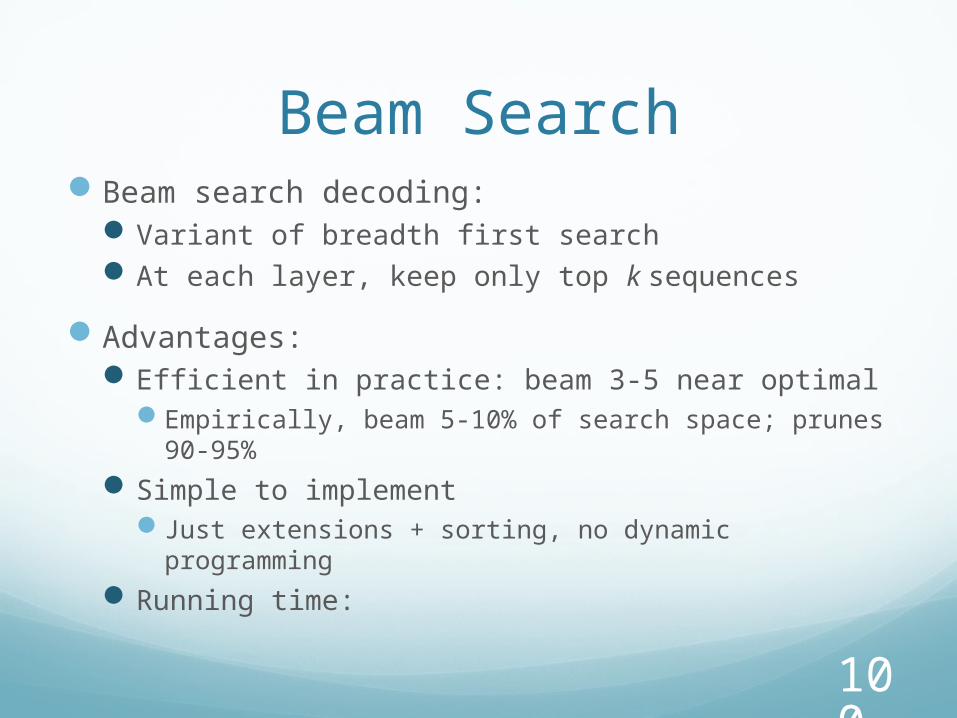
Beam SearchBeam search decoding:
Variant of breadth first searchAt each layer, keep only top k sequences
Advantages:Efficient in practice: beam 3-5 near optimal
Empirically, beam 5-10% of search space; prunes 90-95%
Simple to implementJust extensions + sorting, no dynamic programming
Running time:
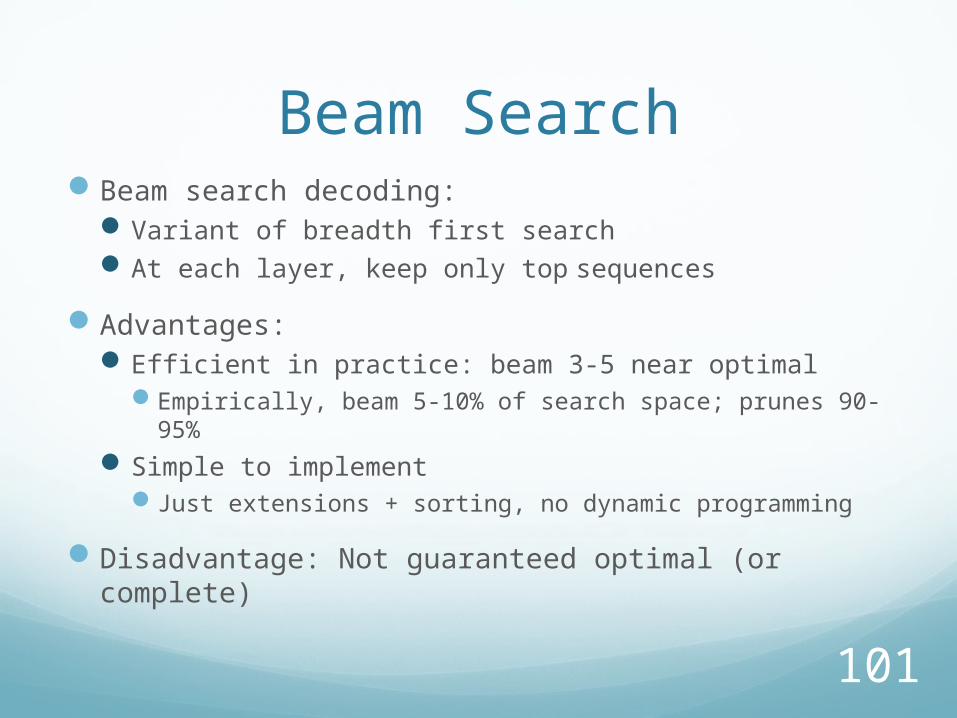
Beam SearchBeam search decoding:
Variant of breadth first searchAt each layer, keep only top sequences
Advantages:Efficient in practice: beam 3-5 near optimal
Empirically, beam 5-10% of search space; prunes 90-95%Simple to implement
Just extensions + sorting, no dynamic programming
Disadvantage: Not guaranteed optimal (or complete)
101

MaxEnt POS TaggingPart of speech tagging by classification:
Feature designword and tag context featuresorthographic features for rare words
102
MaxEnt POS TaggingPart of speech tagging by classification:
Feature designword and tag context featuresorthographic features for rare words
Sequence classification problems:Tag features depend on prior classification
103
MaxEnt POS TaggingPart of speech tagging by classification:
Feature designword and tag context featuresorthographic features for rare words
Sequence classification problems:Tag features depend on prior classification
Beam search decodingEfficient, but inexact
Near optimal in practice
104