ONE-DIMENSIONAL RANDOM WALKS Definition 1. A random walk ...
Matrix Analysis and Algorithms
Andrew Stuart Jochen Voss
4th August 2009
Introduction
The three basic problems we will address in this book are as follows. In all cases we are givenas data a matrix A ∈ Cm×n, with m ≥ n and, for the rst two problems, the vector b ∈ Cm.(SLE) denotes simultaneous linear equations, (LSQ) denotes least squares and (EVP) denoteseigenvalue problem.
(SLE) (m = n)nd x ∈ Cn:
Ax = b
(LSQ) (m ≥ n)nd x ∈ Cn:
minx∈Cn
‖Ax− b‖22
(EVP) (m = n)nd (x, λ) ∈ Cn × C:
Ax = λx, ‖x‖22 = 1
The book contains an introduction to matrix analysis, and to the basic algorithms of numer-ical linear algebra. Further results can be found in many text books. The book of Horn andJohnson [HJ85] is an excellent reference for theoretical results about matrix analysis; see also[Bha97]. The subject of linear algebra, and matrix analysis in particular, is treated in an originaland illuminating fashion in [Lax97]. For a general introduction to the subject of numerical linearalgebra we recommend the book by Trefethen and Bau [TB97]; more theoretical treatments ofthe subject can be found in Demmel [Dem97], Golub and Van Loan [GL96] and in Stoer andBulirsch [SB02]. Higham's book [Hig02] contains a wealth of information about stability andthe eect of rounding errors in numerical algorithms; it is this source that we used for almostall theorems we state concerning backward error analysis. The book of Saad [Saa97] covers thesubject of iterative methods for linear systems. The symmetric eigenvalue problem is analysedin Parlett [Par80].
Acknowledgement
We are grateful to Menelaos Karavelas, Ian Mitchell and Stuart Price for assistance in the type-setting of this material. We are grateful to a variety of students at Stanford University (CS237A)and at Warwick University (MA398) for many helpful comments which have signicantly im-proved the notes.
1
Contents
1 Vector and Matrix Analysis 41.1 Vector Norms and Inner Products . . . . . . . . . . . . . . . . . . . . . . . . . . 41.2 Eigenvalues and Eigenvectors . . . . . . . . . . . . . . . . . . . . . . . . . . . . . 71.3 Dual Spaces . . . . . . . . . . . . . . . . . . . . . . . . . . . . . . . . . . . . . . . 101.4 Matrix Norms . . . . . . . . . . . . . . . . . . . . . . . . . . . . . . . . . . . . . . 111.5 Structured Matrices . . . . . . . . . . . . . . . . . . . . . . . . . . . . . . . . . . 16
2 Matrix Factorisations 192.1 Diagonalisation . . . . . . . . . . . . . . . . . . . . . . . . . . . . . . . . . . . . . 192.2 Jordan Canonical Form . . . . . . . . . . . . . . . . . . . . . . . . . . . . . . . . 222.3 Singular Value Decomposition . . . . . . . . . . . . . . . . . . . . . . . . . . . . . 242.4 QR Factorisation . . . . . . . . . . . . . . . . . . . . . . . . . . . . . . . . . . . . 272.5 LU Factorisation . . . . . . . . . . . . . . . . . . . . . . . . . . . . . . . . . . . . 292.6 Cholesky Factorisation . . . . . . . . . . . . . . . . . . . . . . . . . . . . . . . . . 31
3 Stability and Conditioning 333.1 Conditioning of SLE . . . . . . . . . . . . . . . . . . . . . . . . . . . . . . . . . . 333.2 Conditioning of LSQ . . . . . . . . . . . . . . . . . . . . . . . . . . . . . . . . . . 353.3 Conditioning of EVP . . . . . . . . . . . . . . . . . . . . . . . . . . . . . . . . . . 373.4 Stability of Algorithms . . . . . . . . . . . . . . . . . . . . . . . . . . . . . . . . . 39
4 Complexity of Algorithms 434.1 Computational Cost . . . . . . . . . . . . . . . . . . . . . . . . . . . . . . . . . . 434.2 Matrix-Matrix Multiplication . . . . . . . . . . . . . . . . . . . . . . . . . . . . . 454.3 Fast Fourier Transform . . . . . . . . . . . . . . . . . . . . . . . . . . . . . . . . . 484.4 Bidiagonal and Hessenberg Forms . . . . . . . . . . . . . . . . . . . . . . . . . . . 50
5 Systems of Linear Equations 525.1 Gaussian Elimination . . . . . . . . . . . . . . . . . . . . . . . . . . . . . . . . . . 525.2 Gaussian Elimination with Partial Pivoting . . . . . . . . . . . . . . . . . . . . . 565.3 The QR Factorisation . . . . . . . . . . . . . . . . . . . . . . . . . . . . . . . . . 60
6 Iterative Methods 676.1 Linear Methods . . . . . . . . . . . . . . . . . . . . . . . . . . . . . . . . . . . . . 686.2 The Jacobi Method . . . . . . . . . . . . . . . . . . . . . . . . . . . . . . . . . . . 716.3 The Gauss-Seidel and SOR Methods . . . . . . . . . . . . . . . . . . . . . . . . . 746.4 Nonlinear Methods . . . . . . . . . . . . . . . . . . . . . . . . . . . . . . . . . . . 756.5 The Steepest Descent Method . . . . . . . . . . . . . . . . . . . . . . . . . . . . . 766.6 The Conjugate Gradient Method . . . . . . . . . . . . . . . . . . . . . . . . . . . 78
7 Least Squares Problems 867.1 LSQ via Normal Equations . . . . . . . . . . . . . . . . . . . . . . . . . . . . . . 877.2 LSQ via QR factorisation . . . . . . . . . . . . . . . . . . . . . . . . . . . . . . . 877.3 LSQ via SVD . . . . . . . . . . . . . . . . . . . . . . . . . . . . . . . . . . . . . . 88
2

8 Eigenvalue Problems 938.1 The Power Method . . . . . . . . . . . . . . . . . . . . . . . . . . . . . . . . . . . 958.2 Inverse Iteration . . . . . . . . . . . . . . . . . . . . . . . . . . . . . . . . . . . . 978.3 Rayleigh Quotient Iteration . . . . . . . . . . . . . . . . . . . . . . . . . . . . . . 988.4 Simultaneous Iteration . . . . . . . . . . . . . . . . . . . . . . . . . . . . . . . . . 988.5 The QR Algorithm for Eigenvalues . . . . . . . . . . . . . . . . . . . . . . . . . . 1008.6 Divide and Conquer for Symmetric Problems . . . . . . . . . . . . . . . . . . . . 102
3
Chapter 1
Vector and Matrix Analysis
The purpose of this chapter is to summarise the fundamental theoretical results from linearalgebra to which we will frequently refer, and to provide some basic theoretical tools which we willuse in our analysis. We study vector and matrix norms, inner-products, the eigenvalue problem,orthogonal projections and a variety of special matrices which arise frequently in computationallinear algebra.
1.1 Vector Norms and Inner Products
Denition 1.1. A vector norm on Cn is a mapping ‖ · ‖ : Cn → R satisfying
a) ‖x‖ ≥ 0 for all x ∈ Cn and ‖x‖ = 0 i x = 0,
b) ‖αx‖ = |α|‖x‖ for all α ∈ C, x ∈ Cn, and
c) ‖x+ y‖ ≤ ‖x‖+ ‖y‖ for all x, y ∈ Cn.
Remark. The denition of a norm on Rn is identical, but with Cn replaced by Rn and Creplaced by R.
Examples.
• the p-norm for 1 ≤ p <∞:
‖x‖p =( n∑j=1
|xj |p)1/p
∀x ∈ Cn;
• for p = 2 we get the Euclidean norm:
‖x‖2 =
√√√√ n∑j=1
|xj |2 ∀x ∈ Cn;
• for p = 1 we get
‖x‖1 =n∑j=1
|xj | ∀x ∈ Cn;
• Innity norm: ‖x‖∞ = max1≤j≤n |xj |.
Theorem 1.2. All norms on Cn are equivalent: for each pair of norms ‖ · ‖a and ‖ · ‖b on Cnthere are constants 0 < c1 ≤ c2 <∞ with
c1‖x‖a ≤ ‖x‖b ≤ c2‖x‖a ∀x ∈ Cn.
4
Proof. Using property b) from the dention of a vector norm it suces to consider vectorsx ∈ S =
x ∈ Cn
∣∣ ‖x‖2 = 1. Since ‖ · ‖a is non-zero on all of S we can dene f : S → R
by f(x) = ‖x‖b/‖x‖a. Because the function f is continuous and the set S is compact there arex1, x2 ∈ S with f(x1) ≤ f(x) ≤ f(x2) for all x ∈ S. Setting c1 = f(x1) > 0 and c2 = f(x2)completes the proof.
Remarks.
1. The same result holds for norms on Rn. The proof transfers to this situation withoutchange.
2. We remark that, if A ∈ Cn×n is an invertible matrix and ‖ · ‖ a norm on Cn then ‖ · ‖A :=‖A · ‖ is also a norm.
Denition 1.3. An inner-product on Cn is a mapping 〈 · , · 〉 : Cn × Cn → C satisfying:
a) 〈x, x〉 ∈ R+ for all x ∈ Cn and 〈x, x〉 = 0 i x = 0;
b) 〈x, y〉 = 〈y, x〉 for all x, y ∈ Cn;
c) 〈x, αy〉 = α〈x, y〉 for all α ∈ C, x, y ∈ Cn;
d) 〈x, y + z〉 = 〈x, y〉+ 〈x, z〉 for all x, y, z ∈ Cn;
Remark. Conditions c) and d) above state that 〈 · , · 〉 is linear in the second component. Usingthe rules for inner products we get
〈x+ y, z〉 = 〈x, z〉+ 〈y, z〉 for all x, y, z ∈ Cn
and〈αx, y〉 = α〈x, y〉 for all α ∈ C, x, y ∈ Cn.
The inner product is said to be anti-linear in the rst component.
Example. The standard inner product on Cn is given by
〈x, y〉 =n∑j=1
xjyj ∀x, y ∈ Cn. (1.1)
Denition 1.4. Two vectors x, y are orthogonal with respect to an inner product 〈 · , · 〉 i〈x, y〉 = 0.
Lemma 1.5 (Cauchy-Schwarz inequality). Let 〈 · , · 〉 : Cn×Cn → C be an inner product. Then∣∣〈x, y〉∣∣2 ≤ 〈x, x〉 · 〈y, y〉 (1.2)
for every x, y ∈ Cn and equality holds if and only if x and y are linearly dependent.
Proof. For every λ ∈ C we have
0 ≤ 〈x− λy, x− λy〉 = 〈x, x〉 − λ〈y, x〉 − λ〈x, y〉+ λλ〈y, y〉. (1.3)
For λ = 〈y, x〉/〈y, y〉 this becomes
0 ≤ 〈x, x〉 − 〈x, y〉〈y, x〉〈y, y〉
− 〈y, x〉〈x, y〉〈y, y〉
+〈y, x〉〈x, y〉〈y, y〉
= 〈x, x〉 −∣∣〈x, y〉∣∣2〈y, y〉
and multiplying the result by 〈y, y〉 gives (1.2).If equality holds in (1.2) then x−λy in (1.3) must be 0 and thus x and y are linearly dependent.
If on the other hand x and y are linearly dependent, say x = αy, then λ = 〈y, αy〉/〈y, y〉 = αand x− λy = 0 giving equality in (1.3) and thus in (1.2).
5
Lemma 1.6. Let 〈 · , · 〉 : Cn × Cn → C be an inner product. Then ‖ · ‖ : Cn → R dened by
‖x‖ =√〈x, x〉 ∀x ∈ Cn
is a vector norm.
Proof. a) Since 〈 · , · 〉 is an inner product we have 〈x, x〉 ≥ 0 for all x ∈ Cn, i.e.√〈x, x〉 is real
and positive. Also we get
‖x‖ = 0 ⇐⇒ 〈x, x〉 = 0 ⇐⇒ x = 0.
b) We have
‖αx‖ =√〈αx, αx〉 =
√αα〈x, x〉 = |α| · ‖x‖.
c) Using the Cauchy-Schwarz inequality∣∣〈x, y〉∣∣ ≤ ‖x‖‖y‖ ∀x, y ∈ Cn
from Lemma 1.5 we get
‖x+ y‖2 = 〈x+ y, x+ y〉= 〈x, x〉+ 〈x, y〉+ 〈y, x〉+ 〈y, y〉≤ ‖x‖2 + 2
∣∣〈x, y〉∣∣+ ‖y‖2
≤ ‖x‖2 + 2‖x‖‖y‖+ ‖y‖2
=(‖x‖+ ‖y‖
)2 ∀x, y ∈ Cn.
This completes the proof.
Remark. The angle between two vectors x and y is the unique value ϕ ∈ [0, π] with
cos(ϕ)‖x‖‖y‖ = 〈x, y〉.
When considering the Euclidean norm and inner product on Rn, this denition of angle coincideswith the usual, geometric meaning of angles. In any case, two vectors are orthogonal, if and onlyif they have angle π/2.
We write matrices A ∈ Cm×n as
A =
a11 a12 . . . a1n
a21 a22 . . . a2n
......
...am1 am2 . . . amn
;
we write (A)ij = aij for the ijth entry of A.
Denition 1.7. Given A ∈ Cm×n we dene the adjoint A∗ ∈ Cn×m by(A∗)ij
= aji. (For
A ∈ Rm×n we write AT instead of A∗.)
By identifying the space Cn of vectors with the space Cn×1 of n × 1-matrices, we can takethe adjoint of a vector. Then we can write the standard inner product as
〈x, y〉 = x∗y.
Thus, the standard inner product satises
〈Ax, y〉 = (Ax)∗y = x∗A∗y = 〈x,A∗y〉
for all x ∈ Cn, y ∈ Cm and all A ∈ Cm×n. Unless otherwise specied, we will use 〈 · , · 〉 todenote the standard inner product (1.1) and ‖ · ‖2 to denote the corresponding Euclidean norm.
6
The following families of special matrices will be central in what follows:
Denition 1.8. 1. Q ∈ Cm×n is unitary if Q∗Q = I. (If Q is real then QTQ = I and we sayQ is orthogonal.)
2. A ∈ Cn×n is Hermitian if A∗ = A. (If A is real, we say A is symmetric.)
3. A Hermitian matrix A ∈ Cn×n is positive-denite (resp. positive semi-denite) if x∗Ax =〈Ax, x〉 > 0 (resp. ≥ 0) for all x ∈ Cn \ 0. In this text, whenever we use the terminologypositive-denite or positive semi-denite we are necessarily refering to Hermitian matrices.
Remarks. Unitary matrices have the following properties:
• A matrix Q is unitary, if and only if the columns of Q are orthonormal with respect to thestandard inner-product. In particular unitary matrices cannot have more columns thanrows.
• If Q is a square matrix, Q−1 = Q∗ and thus QQ∗ = I.
• A square matrix Q is unitary, if and only if Q∗ is unitary.
The standard inner product and norm are invariant under multiplication by a unitary matrix:
Theorem 1.9. Let 〈 · , · 〉 denote the standard inner product. Then for any unitary Q ∈ Cm×nand any x, y ∈ Cn we have 〈Qx,Qy〉 = 〈x, y〉 and ‖Qx‖2 = ‖x‖2.
Proof. The rst claim follows from 〈Qx,Qy〉 = 〈x,Q∗Qy〉 = 〈x, y〉 and using the relation ‖x‖2 =〈x, x〉 gives the second claim.
Other inner products with appropriate properties can give rise to other norms; for example,for matrices A which are Hermitian and positive-denite,
〈x, y〉A = 〈x,Ay〉 (1.4)
is an inner product and‖x‖A =
√〈x, x〉A. (1.5)
denes a norm (see Exercise 1-2).
1.2 Eigenvalues and Eigenvectors
Denition 1.10. Given a matrix A ∈ Cn×n, a vector x ∈ Cn is an eigenvector and λ ∈ C is aneigenvalue (also called a right eigenvalue) of A if
Ax = λx and x 6= 0. (1.6)
When x is an eigenvector of A, then for every α 6= 0 the vector αx is an eigenvector for thesame eigenvalue, since both sides of (1.6) are linear in x. Sometimes it is convenient to normalisex by choosing ‖x‖2 = 1. Then the eigenvalue problem is to nd (x, λ) ∈ Cn × C satisfying
Ax = λx and ‖x‖2 = 1.
Denition 1.11. Given a matrix A ∈ Cn×n we dene the characteristic polynomial of A as
ρA(z) := det(A− zI).
Theorem 1.12. A value λ ∈ C is an eigenvalue of the matrix A, if and only if ρA(λ) = 0.
Proof. λ is an eigenvalue of A, if and only if there is an x 6= 0 with (A − λI)x = 0. This isequivalent to the condition that A− λI is singular which in turn is equivalent to det(A− λI) =0.
7
Since ρA is a polynomial of degree n, there will be n (some possibly repeated) eigenvalues,denoted by λ1, . . . , λn and determined by ρA(λk) = 0.
Denition 1.13. An eigenvalue λ has algebraic multiplicity q if q is the largest integer suchthat (z − λ)q is a factor of the characteristic polynomial ρA(z). The geometric multiplicity, r, isthe dimension of the null space of A− λI. An eigenvalue is simple if q = r = 1.
If λ is an eigenvalue of A ∈ Cn×n then det(A− λI) = 0 which implies that det(A∗ − λI) = 0and so (A∗ − λI) has non-trivial null space. Thus there is a vector y (the eigenvector of A∗
corresponding to the eigenvalue λ) with y∗A = λy∗ and y 6= 0.
Denition 1.14. A vector y ∈ Cn with
y∗A = λy∗ and y 6= 0
is known as a left eigenvector of A ∈ Cn×n corresponding to the eigenvalue λ.
Note that, even though the corresponding eigenvalues are the same, the right and left eigen-vectors of a matrix are usually dierent.
Denition 1.15. Matrices A,B ∈ Cn×n are similar, if B = S−1AS with S ∈ Cn×n invertible.The matrix S is a similarity transform.
Remarks. If a matrix A ∈ Cn×n has n linearly independent eigenvectors xi and we arrangethem as columns of the matrix X, then X is invertible. If we let Λ denote a diagonal matrixwith eigenvalues of A on the diagonal, then we may write
AX = XΛ.
By invertibility of X we haveA = XΛX−1. (1.7)
Thus Λ is a similarity transform of A. It reveals the eigenstructure of A and is hence veryuseful in many situations. However, in general a matrix does not have n linearly independenteigenvalues and hence generalizations of this factorization are important. Two which will arisein the next chapter are:
• Jordan Canonical Form: A = SJS−1 (see Theorem 2.7)
• Schur Factorization: A = QTQ∗ (see Theorem 2.2)
These are both similarity transformations which reveal the eigenvalues of A on the diagonalsof J and T , respectively. The Jordan Canonical Form is not stable to perturbations, but theSchur Factorization is. Hence Schur Factorization will form the basis of good algorithms whilethe Jordan Canonical Form is useful for more theoretical purposes, such as dening the matrixexponential eAt.
Theorem 1.16 (Similarity and Eigenvalues). If B is similar to A, then B and A have the sameeigenvalues with the same algebraic and geometric multiplicities.
Proof. Exercise 2-4.
Lemma 1.17. For a simple eigenvalue µ,
dim(ker(A− µI)2
)= 1.
Proof. (Sketch) We prove this in the case where A has n linearly independent eigenvaluesxi all of which correspond to simple eigenvalues λi. Then A may be factorized as in (1.7) withΛ = diagλ1, λ2, . . . , λn. Hence
(A− µI)2 = XΩX−1,
8
where Ω = diag(λ1 − µ)2, (λ2 − µ)2, . . . , (λn − µ)2.Without loss of generality let µ = λ1, noting that λj 6= µ by simplicity. ker(Ω) is one
dimensional, spanned by e1. Hence ker(A− µI)2 is one dimensional by Theorem 1.16The general case can be established by use of the Jordan form (see Theorem 2.7), using the
fact that the Jordan block corresponding to a simple eigenvalue is diagonal.
Theorem 1.18 (Eigenvalue Multiplicities). For any eigenvalue of A ∈ Rn×n the algebraic andgeometric multiplicities q and r respectively satisfy
1 ≤ r ≤ q.
Proof. Let µ be the eigenvalue. Since (A− µI) is non-invertible, its null-space U has dimensionr ≥ 1. Let V ∈ Cn×r have r columns comprising an orthonormal basis for U ; then extend V toV ∈ Cn×n by adding orthonormal columns so that V is unitary. Now
B = V ∗AV =(µI C0 D
),
where I is the r× r identity, C is r× (n− r) and D is (n− r)× (n− r), and B and A are similar.Then
det(B − zI) = det(µI − zI) det(D − zI)= (µ− z)r det(D − zI).
Thus B has algebraic multiplicity ≥ r for B and hence A has algebraic multiplicity ≥ r, byTheorem 1.16.
Denition 1.19. The spectral radius of a matrix A ∈ Cn×n is dened by
ρ(A) = max|λ|∣∣ λ is eigenvalue of A
.
By considering the eigenvectors of a matrix, we can dene an important class of matrices
Denition 1.20. A matrix A ∈ Cn×n is normal i it has n orthogonal eigenvectors.
The importance of this concept lies in the fact, that normal matrices can always be diago-nalised: if Q ∈ Cn×n is a matrix where the columns form an orthonormal system of eigenvectorsand Λ ∈ Cn×n is the diagonal matrix with the corresponding eigenvalues on the diagonal, thenwe have
A = QΛQ∗.
Using this relation, we see that every normal matrix satises A∗A = QΛ∗ΛQ∗ = QΛΛ∗Q∗ =AA∗. In Theorem 2.3 we will see that the condition A∗A = AA∗ is actually equivalent to Abeing normal in the sense of the denition above. Sometimes this alternative condition is usedto dene when a matrix is normal. As a consequence of this equivalence, every Hermitian matrixis also normal.
Let now A be Hermitian and positive denite. Then Ax = λx implies
λ〈x, x〉 = 〈x, λx〉 = 〈x,Ax〉 = 〈Ax, x〉 = 〈λx, x〉 = λ〈x, x〉.
Thus, all eigenvalues of A are real and we can arrange them in increasing order λmin = λ1 ≤· · · ≤ λn = λmax. The following lemma uses λmin and λmax to estimate the values of the norm‖ · ‖A from (1.5) by ‖ · ‖.
Lemma 1.21. Let λmin and λmax be the smallest and largest eigenvalues of a Hermitian, positivedenite matrix A ∈ Cn×n. Then
λmin‖x‖2 ≤ ‖x‖2A ≤ λmax‖x‖2 ∀x ∈ Cn.
9
Proof. Let ϕ1, . . . , ϕn be an orthonormal system of eigenvectors of A with corresponding eigen-values λmin = λ1 ≤ · · · ≤ λn = λmax. By writing x as x =
∑ni=1 ξiϕi we get
‖x‖2 =n∑i=1
|ξi|2
and
‖x‖2A =n∑i=1
λiξ2i .
This gives the upper bound
‖x‖2A ≤n∑i=1
λmaxξ2i ≤ λmax‖x‖2
and similarly we get the lower bound.
1.3 Dual Spaces
Let 〈 · , · 〉 denote the standard inner-product.
Denition 1.22. Given a norm ‖ · ‖ on Cn, the pair (Cn, ‖ · ‖) is a Banach space B. The Banachspace B′, the dual of B, is the pair (Cn, ‖ · ‖B′), where
‖x‖B′ = max‖y‖=1
|〈x, y〉|.
See Exercise 1-5 to deduce that the preceeding denition satises the norm axioms.
Theorem 1.23. The spaces (Cn, ‖ · ‖1) and (Cn, ‖ · ‖∞) are the duals of one another.
Proof. Firstly, we must show‖x‖1 = max
‖y‖∞=1|〈x, y〉|.
This is clearly true for x = 0 and so we consider only x 6= 0. Now
|〈x, y〉| ≤ maxi|yi|
n∑j=1
|xj | = ‖y‖∞‖x‖1,
and thereforemax‖y‖∞=1
|〈x, y〉| ≤ ‖x‖1.
We need to show that this upper-bound is achieved. If yj = xj/|xj | (with the convention thatthis is 0 when xj is 0) then ‖y‖∞ = 1 (since x 6= 0) and
〈x, y〉 =n∑j=1
|xj |2/|xj | =n∑j=1
|xj | = ‖x‖1.
Hence max‖y‖∞=1 |〈x, y〉| = ‖x‖1.Secondly, it remains to show that
‖x‖∞ = max‖y‖1=1
|〈x, y〉|.
We have
|〈x, y〉| ≤ ‖y‖1‖x‖∞⇒ max
‖y‖1=1|〈x, y〉| ≤ ‖x‖∞.
If x = 0 we have equality; if not then, for some k such that |xk| = ‖x‖∞ > 0, choose yj =δjkxk/|xk|. Then
〈x, y〉 = |xk| = ‖x‖∞ and ‖y‖1 = 1.
Thus max‖y‖1=1 |〈x, y〉| = ‖x‖∞.
10
Theorem 1.24. If p, q ∈ (1,∞) with p−1 + q−1 = 1 then the Banach spaces (Cn, ‖ · ‖p) and(Cn, ‖ · ‖q) are the duals of one another.
Proof. See Exercise 1-6.
1.4 Matrix Norms
Since we can consider the space Cm×n of allm×n-matrices to be a copy of them×n-dimensionalvector space Cmn, we can use all vector norms on Cmn as vector norms on the matrices Cm×n.Examples of vector norms on the space of matrices include
• maximum norm: ‖A‖max = maxi,j |aij |
• Frobenius norm: ‖A‖F =(∑m,n
i,j=1 |aij |2) 1
2
• operator norm Cn → Cm: if A ∈ Cm×n,
‖A‖(m,n) = max‖x‖n=1
‖Ax‖m
where ‖ · ‖m is a norm on Cm, and ‖ · ‖n is a norm on Cn. Note that, for any operatornorm,
‖A‖(m,n) = max‖x‖n≤1
‖Ax‖m = max‖x‖n=1
‖Ax‖m = maxx∈Cn\0
‖Ax‖m‖x‖n
.
Sometimes it is helpful to consider special vector norms on a space of matrices, which arecompatible with the matrix-matrix multiplication.
Denition 1.25. A matrix norm on Cn×n is a mapping ‖ · ‖ : Cn×n → R with
a) ‖A‖ ≥ 0 for all A ∈ Cn×n and ‖A‖ = 0 i A = 0,
b) ‖αA‖ = |α|‖A‖ for all α ∈ C, A ∈ Cn×n,
c) ‖A+B‖ ≤ ‖A‖+ ‖B‖ for all A,B ∈ Cn×n.
d) ‖AB‖ ≤ ‖A‖‖B‖ for all A,B ∈ Cn×n.
Remark. Conditions a), b) and c) state that ‖ · ‖ is a vector norm on the vector space Cn×n.Condition d) only makes sense for matrices, since general vectors spaces are not equipped witha product.
Examples of matrix norms include
• p-operator norm Cn → Cn: if A ∈ Cn×n,
‖A‖p = max‖x‖p=1
‖Ax‖p, 1 ≤ p ≤ ∞
The vector operator norm from Cn into Cm reduces to the p-operator norm if n = m andthe p-norm is chosen in the range and image spaces.
Denition 1.26. Given a vector norm ‖ · ‖v on Cn we dene the induced norm ‖ · ‖m on Cn×nby
‖A‖m = maxx 6=0
‖Ax‖v‖x‖v
for all A ∈ Cn×n.
We now show that the induced norm is indeed a norm.
11
Theorem 1.27. The induced norm ‖ · ‖m of a vector norm ‖ · ‖v is a matrix norm with
‖I‖m = 1
and‖Ax‖v ≤ ‖A‖m‖x‖v
for all A ∈ Cn×n and x ∈ Cn.
Proof. a) ‖A‖m ∈ R and ‖A‖m ≥ 0 for all A ∈ Cn×n is obvious from the denition. Also fromthe denition we get
‖A‖m = 0 ⇐⇒ ‖Ax‖v‖x‖v
= 0 ∀x 6= 0
⇐⇒ ‖Ax‖v = 0 ∀x 6= 0 ⇐⇒ Ax = 0 ∀x 6= 0 ⇐⇒ A = 0.
b) For α ∈ C and A ∈ Cn×n we get
‖αA‖m = maxx 6=0
‖αAx‖v‖x‖v
= maxx 6=0
|α|‖Ax‖v‖x‖v
= |α|‖A‖m
c) For A,B ∈ Cn×n we get
‖A+B‖m = maxx 6=0
‖Ax+Bx‖v‖x‖v
≤ maxx 6=0
‖Ax‖v + ‖Bx‖v‖x‖v
≤ maxx 6=0
‖Ax‖v‖x‖v
+ maxx 6=0
‖Bx‖v‖x‖v
= ‖A‖m + ‖B‖m.
Before we check condition d) from the denition of a matrix norm we verify
‖I‖m = maxx 6=0
‖Ix‖v‖x‖v
= maxx 6=0
‖x‖v‖x‖v
= 1
and
‖A‖m = maxy 6=0
‖Ay‖v‖y‖v
≥ ‖Ax‖v‖x‖v
∀x ∈ Cn \ 0
which gives‖Ax‖v ≤ ‖A‖m‖x‖v ∀x ∈ Cn.
d) Using this estimate we nd
‖AB‖m = maxx 6=0
‖ABx‖v‖x‖v
≤ maxx 6=0
‖A‖m‖Bx‖v‖x‖v
= ‖A‖m‖B‖m.
Remarks.
1. Usually one denotes the induced matrix norm with the same symbol as the correspondingvector norm. For the remainder of this text we will follow this convention.
2. As a consequence of theorem 1.27 we can see that not every matrix norm is an inducednorm: If ‖ · ‖m is a matrix norm, then it is easy to check that ‖ · ‖′m = 2‖ · ‖m is a matrixnorm, too. But at most one of these two norms can equal 1 for the identity matrix, andthus the other one cannot be an induced matrix norm.
12
3. Recall that ‖ · ‖A := ‖A · ‖ is a vector norm on Cn whenever ‖ · ‖ is, provided that A isinvertible. The inequality from Theorem 1.27 gives the following upper and lower boundsfor the norm ‖ · ‖ in terms of the original norm:
1‖A−1‖
‖x‖ ≤ ‖x‖A ≤ ‖A‖‖x‖.
Theorem 1.28. The matrix norm induced by the innity norm is the maximum row sum:
‖A‖∞ = max1≤i≤n
n∑j=1
|aij |.
Proof. For x ∈ Cn we get
‖Ax‖∞ = max1≤i≤n
|(Ax)i| = max1≤i≤n
|n∑j=1
aijxj | ≤ max1≤i≤n
n∑j=1
|aij |‖x‖∞
which gives
‖Ax‖∞‖x‖∞
≤ max1≤i≤n
n∑j=1
|aij |
for all x ∈ Cn and thus ‖A‖∞ ≤ max1≤i≤n∑nj=1 |aij |.
For the lower bound choose k ∈ 1, 2, . . . , n such that
max1≤i≤n
n∑j=1
|aij | =n∑j=1
|akj |
and dene x ∈ Cn by xj = akj/|akj | for all j = 1, . . . , n (with the convention that this is 0 whenakj is 0). Then we have ‖x‖∞ = 1 and
‖A‖∞ ≥‖Ax‖∞‖x‖∞
= max1≤i≤n
|n∑j=1
aijakj|akj |
|
≥ |n∑j=1
akjakj|akj |
|
=n∑j=1
|akj |
= max1≤i≤n
n∑j=1
|aij |.
This is the required result.
Theorem 1.29. Let A ∈ Cn×n. Then ‖A∗‖1 = ‖A‖∞ and so
‖A‖1 = ‖A∗‖∞ = max1≤j≤n
n∑i=1
|aij |.
This expression is known as the maximum column sum.
13
Proof. (Sketch)
‖A‖∞ = max‖x‖∞=1
‖Ax‖∞
= max‖x‖∞=1
(max‖y‖1=1
|〈Ax, y〉|)
(Dual denition)
= max‖y‖1=1
(max‖x‖∞=1
|〈Ax, y〉|)
(needs careful justication)
= max‖y‖1=1
(max‖x‖∞=1
|〈x,A∗y〉|)
(denition of A∗)
= max‖y‖1=1
‖A∗y‖1 (Dual denition)
= ‖A∗‖1.
Since (A∗)ij = aji, the result follows.
Remark. This result is readily extended to non-square matrices A ∈ Cm×n.
Recall that the spectral radius of a matrix is dened as
ρ(A) = max|λ|∣∣ λ is eigenvalue of A
.
Theorem 1.30. For any matrix norm ‖ · ‖, any matrix A ∈ Cn×n and any k ∈ N we have
ρ(A)k ≤ ρ(Ak) ≤ ‖Ak‖ ≤ ‖A‖k.
Proof. Let B = Ak. The rst inequality is a consequence of the fact that, whenever x is aneigenvector of A with eigenvalue λ, the vector x is also an eigenvector of B, but with eigenvalueλk. By denition of the spectral radius ρ(B) we can nd an eigenvector x with Bx = λx andρ(B) = |λ|. Let X ∈ Cn×n be the matrix where all n columns are equal to x. Then we haveBX = λX and thus
‖B‖‖X‖ ≥ ‖BX‖ = ‖λX‖ = |λ|‖X‖ = ρ(B)‖X‖.
Dividing by ‖X‖ gives ρ(B) ≤ ‖B‖. The nal inequality follows from property d) in the denitionof a matrix norm.
Theorem 1.31. If A ∈ Cn×n is normal, then
ρ(A)` = ‖A`‖2 = ‖A‖`2 ∀` ∈ N.
Proof. Let x1, . . . , xn be an orthonormal basis composed of eigenvectors of A with correspondingeigenvalues λ1, . . . , λn. Without loss of generality we have ρ(A) = |λ1|.
Let x ∈ Cn. Then we can write
x =n∑j=1
αjxj
and get
‖x‖22 =n∑j=1
|αj |2.
Similarly we nd
Ax =n∑j=1
αjλjxj and ‖Ax‖22 =n∑j=1
|αjλj |2.
14
This shows
‖Ax‖2‖x‖2
=
(∑nj=1 |αjλj |2
)1/2(∑nj=1 |αj |2
)1/2≤(∑n
j=1 |αj |2|λ1|2∑nj=1 |αj |2
)1/2
= |λ1| = ρ(A) ∀x ∈ Cn
and consequently ‖A‖2 ≤ ρ(A).Using Theorem 1.30 we get
ρ(A)` ≤ ‖A`‖2 ≤ ‖A‖`2 ≤ ρ(A)`
for all ` ∈ N. This completes the proof.
Similar methods to those used in the proof of the previous result yield the following theorem.
Theorem 1.32. For all matrices A ∈ Cm×n
‖A‖22 = ρ(A∗A).
Proof. See Exercise 1-9.
The matrix 2-norm has the special property that it is invariant under multplication by aunitary matrix. This is the analog of Theorem 1.9 for vector norms.
Theorem 1.33. For all matrices A ∈ Cm×n and unitary matrices U ∈ Cm×m, V ∈ Cn×n
‖UA‖2 = ‖A‖2, ‖AV ‖2 = ‖A‖2.
Proof. The rst result follows from the previous theorem, after noting that (UA)∗(UA) =A∗U∗UA = A∗A. Because (AV )∗(AV ) = V ∗(A∗A)V and because V ∗(A∗A)V is a similaritytransformation of A∗A the second result also follows from the previous theorem.
Let A,B ∈ Cm×n. In the following it will be useful to employ the notation |A| to denote thematrix with entries (|A|)ij = |aij | and the notation |A| ≤ |B| as shorthand for |aij | ≤ |bij | forall i, j.
Lemma 1.34. If two matrices A,B ∈ Cm×n satisfy |A| ≤ |B| then ‖A‖∞ ≤ ‖B‖∞ and ‖A‖1 ≤‖B‖1. Furthermore ‖|AB|‖∞ ≤ ‖|A||B|‖∞.
Proof. For the rst two observations, it suces to prove the rst result since ‖A‖1 = ‖A∗‖∞ and|A| ≤ |B| implies that |A∗| ≤ |B∗|. The rst result is a direct consequence of the representationof the ∞-norm and 1-norm from theorems 1.28 and 1.29. To prove the last result note that
(|AB|)ij = |∑k
AikBkj |
≤∑k
|Aik||Bkj |
= (|A||B|)ij .
The rst result completes the proof.
Lemma 1.35. Let A,B ∈ Cn×n. Then
‖A‖max ≤ ‖A‖∞ ≤ n‖A‖max,
‖AB‖max ≤ ‖A‖∞‖B‖max,
‖AB‖max ≤ ‖A‖max‖B‖1.
15
Proof. Exercise 1-8.
Denition 1.36. The outer product of two vectors a, b ∈ Cn is the matrix a⊗ b ∈ Cn×n denedby
(a⊗ b)c = (b∗c)a = 〈b, c〉a ∀c ∈ Cn.
We sometimes write a⊗ b = ab∗. The ijth entry of the outer product is (a⊗ b)ij = aibj .
Denition 1.37. Let S be a subspace of Cn. Then the orthogonal complement of S is denedby
S⊥ = x ∈ Cn | 〈x, y〉 = 0 ∀y ∈ S.
The orthogonal projection onto S, P , can be dened as follows: let yiki=1 be an orthonormalbasis for S, then
Px =k∑j=1
〈yj , x〉yj =( k∑j=1
yjy∗j
)x =
( k∑j=1
yj ⊗ yj)x.
Theorem 1.38. P is a projection, that is P 2 = P . Furthermore, if P⊥ = I − P , then P⊥ isthe orthogonal projection onto S⊥.
Proof. Extend yiki=1 to a basis for Cn, denoted yini=1, noting that S⊥ = span yk+1, . . . , yn.
Any x ∈ Cn can be written uniquely as
x =n∑j=1
〈yj , x〉yj ,
and so
Px =k∑j=1
〈yj , x〉yj ,
found by truncating to k terms. Clearly truncating again leaves the expression unchanged:
P 2x =k∑j=1
〈yj , x〉yj = Px, ∀x ∈ Cn.
Now (I − P )x = P⊥x =∑nj=k+1〈yj , x〉yj , proving the second result.
1.5 Structured Matrices
Denition 1.39. A matrix A ∈ Cn×n is
diagonal if aij = 0 i 6= j
(strictly) upper-triangular if aij = 0 i > j (≥ )(strictly) lower-triangular if aij = 0 i < j (≤ )
upper Hessenberg if aij = 0 i > j + 1upper bidiagonal if aij = 0 i > j& i < j − 1
tridiagonal if aij = 0 i > j + 1 & i < j − 1
Denition 1.40. A matrix P ∈ Rn×n is called a permutation matrix if every row and everycolumn contains n− 1 zeros and 1 one.
16
Remarks.
1. If P is a permutation matrix, then we have
(PTP )ij =n∑k=1
pkipkj = δij
and thus PTP = I. This shows that permutation matrices are orthogonal.
2. If π : 1, . . . , n → 1, . . . , n is a permutation, then the matrix P = (pij) with
pij =
1 if j = π(i) and0 else
is a permutation matrix. Indeed every permutation matrix is of this form. In particularthe identity matrix is a permutation matrix.
3. If P is the permutation matrix corresponding to the permutation π, then (P−1)ij = 1 if andonly if j = π−1(i). Thus the permutation matrix P−1 corresponds to the permutation π−1.
4. We get
(PA)ij =n∑k=1
pikakj = aπ(i),j
for all i, j ∈ 1, . . . , n. This shows that multiplying a permutation matrix from the leftreorders the rows of A. Furthermore we have
(AP )ij =n∑k=1
aikpkj = ai,π−1(j)
and hence multiplying a permutation matrix from the right reorders the columns of A.
5. If P is a permutation matrix, then PT is also a permutation matrix.
Bibliography
Excellent treatments of matrix analysis may be found in [Bha97] and [HJ85]. More advancedtreatment of the subject includes [Lax97]. Theorem 1.16 and Lemma 1.17 are proved in [Ner71].The proof of Theorem 1.24 may be found in [Rob01]. Theorem 1.32 is proved in the solutionsfor instructors.
Exercises
Exercise 1-1. Show that the following relations hold for all x ∈ Cn:a) ‖x‖2 ≤ ‖x‖1 ≤
√n‖x‖2,
b) ‖x‖∞ ≤ ‖x‖2 ≤√n‖x‖∞ and
c) ‖x‖∞ ≤ ‖x‖1 ≤ n‖x‖∞.
Exercise 1-2. Prove that, for Hermitian positive denite A, equations (1.4) and (1.5) dene aninner-product and norm, respectively.
Exercise 1-3. For matrices in Rm×n prove that
‖A‖max ≤ ‖A‖F ≤√mn‖A‖max.
17
Exercise 1-4. Dene an inner product 〈 · , · 〉 on matrices in Rn×n such that
‖A‖2F = 〈A,A〉.
Exercise 1-5. Prove that the norm ‖ · ‖B′ appearing in Denition 1.22 is indeed a norm.
Exercise 1-6. Prove Theorem 1.24.
Exercise 1-7. Show that ‖A‖max = maxi,j |aij | for all A ∈ Cn×n denes a vector norm on thespace of n× n-matrices, but not a matrix norm.
Exercise 1-8. Prove Lemma 1.35.
Exercise 1-9. Show that ‖A‖22 = ρ(ATA) for every matrix A ∈ Rn×n (this is the real versionof Theorem 1.32).
Exercise 1-10. For A ∈ Rn×n recall the denition of |A|, namely (|A|)ij = |aij |. Show that
‖|A|‖ = ‖A‖
holds in the Frobenius, innity and 1-norms. Is the result true in the Euclidean norm? Justifyyour assertion.
Exercise 1-11. Let ‖ · ‖ be an operator norm. Prove that if ‖X‖ < 1, then
• I −X is invertible,
• the series∑∞i=0X
i converges, and
• (I −X)−1 =∑∞i=0X
i.
Moreover, prove that in the same norm
‖(I −X)−1‖ ≤ (1− ‖X‖)−1.
Exercise 1-12. Let K be a matrix in Rn×n with non-negative entries and let f, g be two vectorsin Rn with strictly positive entries which satisfy
(Kf)i/gi < λ, (KT g)i/fi < µ ∀i ∈ 1, . . . , n.
Prove that ‖K‖22 ≤ λµ.
Exercise 1-13. Let A ∈ Rk×l, B ∈ Rl×m and C ∈ Rm×m. Here k ≥ l. If A and C areorthogonal, that is if CTC = I (the identity on Rm) and ATA = I (the identity on Rl) thenshow that ‖ABC‖2 = ‖B‖2.
Exercise 1-14. Prove that the Frobenius norm of a matrix is unchanged by multplication byunitary matrices. This is an analogue of Theorem 1.33.
Exercise 1-15. Show that for every vector norm ‖ · ‖ on Rn×n there is a number λ > 0 suchthat
‖A‖λ = λ‖A‖ A ∈ Rn×n
denes a matrix norm.
18
Chapter 2
Matrix Factorisations
In this chapter we present various matrix factorisations. These are of interest in their own right,and also because they form the basis for many useful numerical algorithms.
There are two groups of results presented in this chapter. The rst kind of results factorisesa matrix A ∈ Cn×n as
A = SAS−1
where, typically, A is of a simpler form than the original matrix A. Results of this type arematrix diagonalisations and the Jordan canonical form. These factorisations are useful, becauseproperties of A are often easier to understand than properties of A and often questions about Acan be reduced to questions about A. For example, since Ax = λx implies A(S−1x) = λ(S−1x),the matrices A and A have the same eigenvalues (but dierent eigenvectors). These factorisationsare typically used in proofs.
The second group of results, including the QR factorisation and LU factorisation, just splitsa matrix A into two, simpler parts:
A = BC
where B and C are matrices of a simpler form than A is, for example triangular matrices. Thesefactorisations typically form the basis of numerical algorithms, because they allow to split onecomplicated problem into two simpler ones. This strategy will be used extensively in the laterchapters of this text.
2.1 Diagonalisation
A matrix A ∈ Cn×n is diagonalised by nding a unitary matrix Q ∈ Cn×n and a diagonal matrixD ∈ Cn×n such that
A = QDQ∗.
Since this implies AQ = DQ we see, by considering the individual columns of this matrixequation, that the diagonal elements ofD are the eigenvalues of A and the (orthonormal) columnsof Q are the corresponding eigenvectors. This insight has several consequences: Firstly, a matrixcan be diagonalised if and only if it has a complete, orthonormal system of eigenvectors. And,secondly, there can be no direct algoritms to diagonalise a matrix, since the eigenvalues of amatrix in general cannot be found exactly in nite time (see the discussion around Theorem 8.2).Thus, diagonalisation will be mostly useful as a tool in our proofs and not as part of an algorithm.
The basic result in this section is the Schur triangularisation of a matrix; diagonalisation willfollow from this. The next lemma is key in proving the Schur factorisation.
Lemma 2.1. For all A ∈ Cn×n satisfying dim(range(A)) = k ≤ n, there is an orthonormal sety1 . . . , yk ⊆ range(A) with the property that Ayl ∈ spany1, . . . , yl for l = 1, . . . , k.
Proof. If k = 1, then there is a y1 ∈ Cn with ‖y1‖2 = 1 which spans range(A). ClearlyAy1 ∈ range(A) = spany1.
19
For induction assume that we have the result for some k < n. Let A satisfy dim(range(A)) =k+1. Choose y1 to be an eigenvector of A with ‖y1‖2 = 1. Let P denote the orthogonal projectiononto spany1 and P⊥ = I − P . Dene A⊥ = P⊥A and note that dim(range(A⊥)) = k. By theinductive hypothesis, there is an orthonormal set y2, . . . , yk+1 ⊆ range(A⊥) with the property
A⊥yl ∈ spany2, . . . , yl l = 2, . . . , k + 1.
Furthermore we have that y1 is orthogonal to spany2, . . . , yk. Consider the set y1, . . . , yk+1.Note that Ay1 = λy1. Also
Ayl = (PA+ P⊥A)yl = PAyl +A⊥yl.
Since PAyl ∈ spany1 and A⊥yl ∈ spany2, . . . , yl we obtain
Ayl ∈ spany1, . . . , yl,
as required.
Theorem 2.2 (Schur Factorisation). For any A ∈ Cn×n, there is a unitary Q ∈ Cn×n and anupper triangular T ∈ Cn×n such that
A = QTQ∗.
Proof. Let k = dim(range(A)), and construct orthonormal vectors y1, . . . , yk as in Lemma 2.1.Since dim
(range(A)⊥
)= n− k, we can nd an orthonormal basis yk+1, . . . , yn of range(A)⊥.
Then yq, . . . , yn is an orthonormal basis of Cn and
Ayl ∈ range(A) = spany1, . . . , yk ⊆ spany1, . . . , yl
for l = k + 1, . . . , n. We also have Ayl ∈ spany1, . . . , yl for l = 1, . . . , k and thus
Ayl =l∑
j=1
tjlyj , l = 1, . . . , n.
Letting Q =(y1 · · · yn
)and dening T by (T )ij = tij for i ≤ j and (T )ij = 0 for i > j we obtain
AQ = QT as required.
Theorem 2.3 (Normal Diagonalisation). If A ∈ Cn×n satises A∗A = AA∗, then there isunitary Q ∈ Cn×n and diagonal D ∈ Cn×n such that A = QDQ∗.
Proof. By Schur factorisation, there is T upper triangular and Q unitary such that
A = QTQ∗,
and it suces to show that T is diagonal.We have
A∗A = QT ∗TQ∗ and QTT ∗Q∗ = AA∗,
and since A is normal we deduce that T ∗T = TT ∗. Now
(T ∗T )ij =∑k
(T ∗)ik(T )kj =∑k
(T )ki(T )kj ,
so that
(T ∗T )ii =∑k
|tki|2 =i∑
k=1
|tki|2.
Similarly,
(TT ∗)ii =n∑k=i
|tik|2.
20
We now prove that T is diagonal by equating these expressions and using induction.
i = 1 : |t11|2 =n∑k=1
|t1k|2,
and so t1k = 0 for k = 2, . . . , n.Assume for induction in m that tlk = 0 for l = 1, . . . ,m− 1 and all k 6= l. Note that we have
proved this for m = 2. Then
(T ∗T )mm =m∑k=1
|tkm|2 = |tmm|2 (by induction hyp.)
(TT ∗)mm =n∑
k=m
|tmk|2 = |tmm|2 +n∑
k=m+1
|tmk|2,
and so tmk = 0 for k = m + 1, . . . , n. Also, tmk = 0 for k = 1, . . . ,m − 1 since T is uppertriangular. Thus
tmk = 0 k 6= m
and tlk = 0 l = 1, . . . ,m, k 6= l,
and the induction is complete.
Remark. In the situation of the preceeding theorem, the diagonal elements of D are theeigenvalues of A and the columns of Q are corresponding eigenvectors. Since Q is unitary, theeigenvectors are orthogonal and thus the matrix A is normal. When combined with the discussionafter denition 1.20 this shows that a matrix A is normal if and only if A∗A = AA∗.
Theorem 2.4 (Hermitian Diagonalisation). If A ∈ Cn×n is Hermitian, then there exists aunitary matrix Q ∈ Cn×n and diagonal Λ ∈ Rn×n such that A = QΛQ∗.
Proof. Since Hermitian matrices are normal, A can be factorised in the required form withΛ ∈ Cn×n diagonal by Theorem 2.3. It remains to show that Λ is real. We have
AQ = QΛ,
and hence, if q1, . . . , qn are the columns of Q, we get Aqi = λiqi and ‖qi‖ = 1. This implies
λi = 〈qi, λiqi〉 = 〈qi, Aqi〉 = 〈Aqi, qi〉 = 〈λiqi, qi〉 = λi
for i = 1, . . . , n as required.
To illustrate the usefulness of Hermitian diagonalisation, we consider the following applica-tion.
Lemma 2.5. Let A ∈ Cn×n be Hermitian and positive denite. Then there is a Hermitian,positive denite matrix A1/2 ∈ Cn×n, the square root of A, such that A = A1/2A1/2.
Proof. Since A ∈ Cn×n is positive-denite, we have
λi‖xi‖22 = 〈xi, Axi〉 > 0
for all eigenpairs (xi, λi) and thus all eigenvalues are positive.By Theorem 2.4 we have
A = QΛQ∗
with λ = diag(λ1, . . . , λn). Since all λi ≥ 0, we may dene Λ1/2 = diag(√λ1, . . . ,
√λn) and this
is real. Now deneA1/2 = QΛ1/2Q∗. (2.1)
Then A1/2A1/2 = QΛ1/2Λ1/2Q∗ = QΛQ∗ = A as required and, since√λi > 0 for all i = 1, . . . , n,
the matrix A1/2 is Hermitian, positive denite.
21
Remarks.
• A real, positive number λ has two distinct square roots,√λ and −
√λ. Similarly, a Hermi-
tian, positive denite matrix A ∈ Cn×n has 2n distinct square roots, obtained by choosingall possible combination of signs in front of the square roots on the diagonal of Λ1/2 in (2.1).The square root constructed in the lemma is the only positive one.
• The same principle used to construct the square root of a matrix here, can be used toconstruct many dierent functions of a Hermitian matrix: one diagonalises the matrix andapplies the function to the eigenvalues on the diagonal.
2.2 Jordan Canonical Form
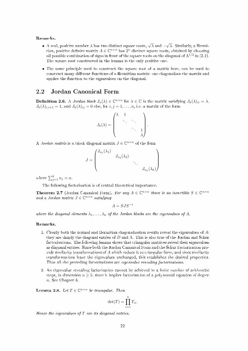
Denition 2.6. A Jordan block Jn(λ) ∈ Cn×n for λ ∈ C is the matrix satisfying Jk(λ)ii = λ,Jk(λ)i,i+1 = 1, and Jk(λ)ij = 0 else, for i, j = 1, . . . , n, i.e. a matrix of the form
Jk(λ) =
λ 1
. . .. . .
. . . 1λ
.
A Jordan matrix is a block diagonal matrix J ∈ Cn×n of the form
J =
Jn1(λ1)
Jn2(λ2). . .
Jnk(λk)
where
∑kj=1 nj = n.
The following factorisation is of central theoretical importance.
Theorem 2.7 (Jordan Canonical Form). For any A ∈ Cn×n there is an invertible S ∈ Cn×nand a Jordan matrix J ∈ Cn×n satisfying
A = SJS−1
where the diagonal elements λ1, . . . , λk of the Jordan blocks are the eigenvalues of A.
Remarks.
1. Clearly both the normal and Hermitian diagonalisation results reveal the eigenvalues of A:they are simply the diagonal entries of D and Λ. This is also true of the Jordan and Schurfactorisations. The following lemma shows that triangular matrices reveal their eigenvaluesas diagonal entries. Since both the Jordan Canonical Form and the Schur Factorisation pro-vide similarity transformations of A which reduce it to triangular form, and since similaritytransformations leave the eigenvalues unchanged, this establishes the desired properties.Thus all the preceding factorisations are eigenvalue revealing factorisations.
2. An eigenvalue revealing factorisation cannot be achieved in a nite number of arithmeticsteps, in dimension n ≥ 5, since it implies factorisation of a polynomial equation of degreen. See Chapter 8.
Lemma 2.8. Let T ∈ Cn×n be triangular. Then
det(T ) =n∏i=1
Tii.
Hence the eigenvalues of T are its diagonal entries.
22
Proof. Let Tj ∈ Cj×j be upper triangular:
Tj =(a b∗
0 Tj−1
),
a ∈ C, b, 0 ∈ Cj−1,
Tj−1 ∈ C(j−1)×(j−1) upper triangular.
Then detTj = adet(Tj−1). By induction,
det(T ) =n∏i=1
Tii.
Eigenvalues of T are λ such that det(T −λI) = 0. Now T −λI is triangular with diagonal entriesTii − λ, therefore
det(T − λI) =n∏i=1
(Tii − λ).
Hence det(T − λi) = 0 if and only if λi = Tii for some i = 1, . . . , n.
As an example of the central theoretical importance of the Jordan normal form we now provea useful lemma showing that a matrix norm can be constructed which, for a given matrix A, hasnorm arbitrarily close to the spectral radius.
Denition 2.9. A δ-Jordan block Jδn(λ) ∈ Cn×n for λ ∈ C is the matrix satisfying Jδk(λ)ii = λ,Jδk(λ)i,i+1 = δ, and Jδk(λ)ij = 0 else, for i, j = 1, . . . , n. A δ-Jordan matrix is a block diagonalmatrix Jδ ∈ Cn×n of the form
J =
Jδn1
(λ1)Jδn2
(λ2). . .
Jδnk(λk)
where
∑kj=1 nj = n.
Lemma 2.10. Let A ∈ Cn×n and δ > 0. Then there is a vector norm ‖ · ‖S on Cn such thatthe induced matrix norm satises ρ(A) ≤ ‖A‖S ≤ ρ(A) + δ.
Proof. From Theorem 1.30 we already know ρ(A) ≤ ‖A‖ for every matrix norm ‖ · ‖. Thus weonly have to show the second inequality of the claim.
Let J = S−1AS be the Jordan Canonical Form of A and Dδ = diag(1, δ, δ2, . . . , δn−1). Then
(SDδ)−1A(SDδ) = D−1δ JDδ = Jδ.
Dene a vector norm ‖ · ‖S on Cn by
‖x‖S =∥∥(SDδ)−1x
∥∥∞
for all x ∈ Cn. Then the induced matrix norm satises
‖A‖S = maxx 6=0
‖Ax‖S‖x‖S
= maxx 6=0
‖(SDδ)−1Ax‖∞‖(SDδ)−1x‖∞
= maxy 6=0
‖(SDδ)−1A(SDδ)y‖∞‖y‖∞
=∥∥(SDδ)−1A(SDδ)‖∞
= ‖Jδ‖∞.
Since we know the ‖ · ‖∞-matrix norm from Theorem 1.28 and we have calculated the explicitform of the matrix (SDδ)−1A(SDδ) above, this is easy to evaluate. We get ‖A‖ ≤ maxi |λi|+δ =ρ(A) + δ. This completes the proof.
23
Remark. In general, ρ( · ) is not a norm. But note that if the Jordan matrix J is diagonal thenδ = 0 and we can deduce the existence of a norm in which ‖A‖S = ρ(A). This situation ariseswhenever A is diagonalisable.
2.3 Singular Value Decomposition
The singular value decomposition is based on the fact that, for any matrix A, it is possible tond a set of real positive σi and vectors ui, vi such that
Avi = σiui.
The σi are known as singular values and, in some applications, are more useful than eigenvalues.This is because the singular values exist even for non-square matrices, because they are alwaysreal, and because the ui and vi always can be chosen orthogonal. Furthermore, the singularvalue decomposition is robust to perturbations, unlike the Jordan canonical form.
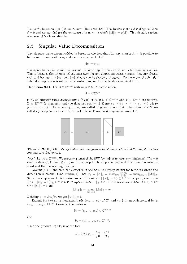
Denition 2.11. Let A ∈ Cm×n with m,n ∈ N. A factorisation
A = UΣV ∗
is called singular value decomposition (SVD) of A, if U ∈ Cm×m and V ∈ Cn×n are unitary,Σ ∈ Rm×n is diagonal, and the diagonal entries of Σ are σ1 ≥ σ2 ≥ · · · ≥ σp ≥ 0 wherep = min(m,n). The values σ1, . . . , σp are called singular values of A. The columns of U arecalled left singular vectors of A, the columns of V are right singular vectors of A.
A = U · Σ · V ∗
Theorem 2.12 (SVD). Every matrix has a singular value decomposition and the singular valuesare uniquely determined.
Proof. Let A ∈ Cm×n. We prove existence of the SVD by induction over p = min(m,n). If p = 0the matrices U , V , and Σ are just the appropriately shaped empty matrices (one dimension iszero) and there is nothing to show.
Assume p > 0 and that the existence of the SVD is already known for matrices where one
dimension is smaller than min(m,n). Let σ1 = ‖A‖2 = maxx 6=0‖Ax‖2‖x‖2 = max‖x‖2=1 ‖Ax‖2.
Since the map v 7→ Av is continuous and the set x | ‖x‖2 = 1 ⊆ Cn is compact, the imageAx | ‖x‖2 = 1 ⊆ Cm is also compact. Since ‖ · ‖2 : Cn → R is continuous there is a v1 ∈ Cnwith ‖v1‖2 = 1 and
‖Av1‖2 = max‖x‖2=1
‖Ax‖2 = σ1.
Dening u1 = Av1/σ1 we get ‖u1‖2 = 1.Extend v1 to an orthonormal basis v1, . . . , vn of Cn and u1 to an orthonormal basis
u1, . . . , um of Cm. Consider the matrices
U1 = (u1, . . . , um) ∈ Cm×m
andV1 = (v1, . . . , vn) ∈ Cn×n.
Then the product U∗1AV1 is of the form
S = U∗1AV1 =(σ1 w∗
0 B
)
24
with w ∈ Cn−1, 0 ∈ Cm−1 and B ∈ C(m−1)×(n−1).For unitary matrices U we have ‖Ux‖2 = ‖x‖2 and thus
‖S‖2 = maxx 6=0
‖U∗1AV1x‖2‖x‖2
= maxx 6=0
‖AV1x‖2‖V1x‖2
= ‖A‖2 = σ1.
On the other hand we get∥∥∥S (σ1
w
)∥∥∥2
=∥∥∥(σ2
1 + w∗wBw
)∥∥∥2≥ σ2
1 + w∗w =(σ2
1 + w∗w)1/2∥∥∥(σ1
w
)∥∥∥2
and thus ‖S‖2 ≥ (σ21 + w∗w)1/2. Thus we conclude that w = 0 and thus
A = U1SV∗1 = U1
(σ1 00 B
)V ∗1 .
By the induction hypothesis the (m−1)×(n−1)-matrix B has a singular value decomposition
B = U2Σ2V∗2 .
Then
A = U1
(1 00 U2
)·(σ1 00 Σ2
)·(
1 00 V ∗2
)V ∗1
is a SVD of A and existence of the SVD is proved.Uniqueness of the largest singular value σ1 holds, since σ1 is uniquely determined by the
relation
‖A‖2 = maxx 6=0
‖UΣV ∗x‖2‖x‖2
= maxx 6=0
‖Σx‖2‖x‖2
= σ1.
Uniqueness of σ2, . . . , σn follows by induction as above.
The penultimate line of the proof shows that, with the ordering of singular values as dened,we have the following:
Corollary 2.13. For any matrix A ∈ Cm×n we have ‖A‖2 = σ1.
Remarks.
1. Inspection of the above proof reveals that for real matrices A the matrices U and V arealso real.
2. Ifm > n then the lastm−n columns of U do not contribute to the factorisation A = UΣV ∗:
A = U · Σ · V ∗
Hence we can also write A as A = U ΣV ∗ where U ∈ Cm×n consists of the rst n columnsof U and Σ ∈ Cn×n consists of the rst n rows of Σ. This factorisation is called the reducedsingular value decomposition (reduced SVD) of A.
3. Since we have A∗A = V Σ∗U∗UΣV ∗ = V Σ∗ΣV ∗ and thus A∗A · V = V · Σ∗Σ, we ndA∗Avj = σ2
j vj for the columns v1, . . . , vn of V . This shows that the vectors vj are eigen-
vectors of A∗A with eigenvalues σ2j .
4. From the proof we see that we can get the ‖ · ‖2-norm of a matrix from its SVD: we have‖A‖2 = σ1.
25
Theorem 2.14. For m ≥ n the SVD has the following properties:
1. If A ∈ Rn×n is Hermitian then A = QΛQ∗ with Λ = diag(λ1, . . . , λn) and Q =(q1 · · · qn
).
An SVD of A may be found in the form A = UΣV T with U = Q, Σ = |Λ|, and
V =(v1 · · · vn
), vi = sgn(λi)qi.
2. The eigenvalues of A∗A are σ2i and the eigenvectors of A∗A are the right singular vectors
vi.
3. The eigenvalues of AA∗ are σ2i and (m − n) zeros. The (right) eigenvectors of AA∗ cor-
responding to eigenvalues σ2i are the left singular vectors ui corresponding to the singular
values σi.
Proof. 1. By denition.
2. We have, from the reduced SVD,
A = U ΣV ∗ =⇒ A∗A = V Σ2V ∗ ∈ Rn×n
Since V is orthogonal and Σ2 = diag(σ21 , . . . , σ
2n), the result follows.
3. We haveA = UΣV ∗ =⇒ AA∗ = UΣΣ∗U∗
where U ∈ Rm×(m−n) is any matrix such that [U U ] ∈ Rm×m is orthogonal. The resultthen follows since
ΣΣ∗ =(
Σ2 00 0
).
For the rest of this section let A ∈ Cm×n be a matrix with singular value decompositionA = UΣV ∗ and singular values σ1 ≥ · · · ≥ σr > 0 = · · · = 0. To illustrate the usefulness of theSVD we prove several fundamental results about it.
Theorem 2.15. The rank of A is equal to r.
Proof. Since U and V ∗ are invertible we have rank(A) = rank(Σ) = r.
Theorem 2.16. We have range(A) = spanu1, . . . , ur and ker(A) = spanvr+1, . . . , vn.
Proof. Since Σ is diagonal and V ∗ is invertible we have
range(ΣV ∗) = range(Σ) = spane1, . . . , er ⊆ Cm.
This showsrange(A) = range(UΣV ∗) = spanu1, . . . , ur ⊆ Cm.
We also haveker(A) = ker(UΣV ∗) = ker(ΣV ∗).
Since V is orthogonal we can conclude
ker(A) = spanvr+1, . . . , vn ⊆ Cn.
26
Theorem 2.17 (The SVD and Eigenvalues). Let A ∈ Rn×n be invertible with SVD A = UΣV T .If
H =(
0 AT
A 0
)∈ R2n×2n
and
U = (u1 · · · un)V = (v1 · · · vn)Σ = diag(σ1, . . . , σn)
then H has
• 2n eigenvalues ±σini=1
• eigenvectors
1√2
(vi±ui
) ∣∣ i = 1, . . . , n
Proof. If Hx = λx with x = (yT , zT )T then
AT z = λy
Ay = λz.
Hence
AT (λz) = λ2y
and ATAy = λ2y.
Thus λ2 ∈ σ21 , . . . , σ
2n and so the 2n eigenvalues of H are drawn from the set
±σ1, . . . ,±σn.
Note thatATU = V Σ, AV = UΣ
and soAvi = σiui, A
Tui = σivi.
The eigenvalue problem for H may be written as
Ay = λz, AT z = λy.
Hence, taking λ = ±σi, we obtain 2n solutions of the eigenvalue problem given by
(yT , zT ) =1√2
(vi,±ui).
This exhibits a complete set of 2n eigenvectors for H.
2.4 QR Factorisation
The SVD factorisation, like the four preceding it, reveals eigenvalues; hence it cannot be achievedin a nite number of steps. The next three factorisations, QR, LU and Cholesky do not revealeigenvalues and, as we will show in later chapters, can be achieved in a polynomial numberof operations, with respect to dimension n. Recall the following classical algorithm for theconstruction of an orthonormal basis from the columns of a matrix A.
27
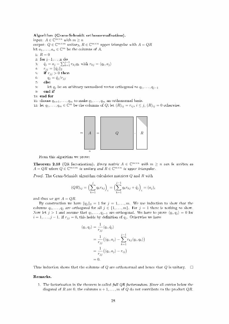
Algorithm (Gram-Schmidt orthonormalisation).input: A ∈ Cm×n with m ≥ noutput: Q ∈ Cm×m unitary, R ∈ Cm×n upper triangular with A = QRlet a1, . . . , an ∈ Cm be the columns of A.
1: R = 02: for j=1,. . . ,n do3: qj = aj −
∑j−1k=1 rkjqk with rkj = 〈qk, aj〉
4: rjj = ‖qj‖25: if rjj > 0 then6: qj = qj/rjj7: else8: let qj be an arbitrary normalised vector orthogonal to q1, . . . , qj−1
9: end if10: end for11: choose qn+1, . . . , qm to make q1, . . . , qm an orthonormal basis.12: let q1, . . . , qm ∈ Cm be the columns of Q; let (R)ij = rij , i ≤ j, (R)ij = 0 otherwise.
Am
n
= Q · R
From this algorithm we prove:
Theorem 2.18 (QR factorisation). Every matrix A ∈ Cm×n with m ≥ n can be written asA = QR where Q ∈ Cm×m is unitary and R ∈ Cm×n is upper triangular.
Proof. The Gram-Schmidt algorithm calculates matrices Q and R with
(QR)ij =( j∑k=1
qkrkj
)i
=(j−1∑k=1
qkrkj + qj
)i
= (aj)i
and thus we get A = QR.By construction we have ‖qj‖2 = 1 for j = 1, . . . ,m. We use induction to show that the
columns q1, . . . , qj are orthogonal for all j ∈ 1, . . . ,m. For j = 1 there is nothing to show.Now let j > 1 and assume that q1, . . . , qj−1 are orthogonal. We have to prove 〈qi, qj〉 = 0 fori = 1, . . . , j − 1. If rjj = 0, this holds by denition of qj . Otherwise we have
〈qi, qj〉 =1rjj〈qi, qj〉
=1rjj
(〈qi, aj〉 −
j−1∑k=1
rkj〈qi, qk〉)
=1rjj
(〈qi, aj〉 − rij
)= 0.
Thus induction shows that the columns of Q are orthonormal and hence that Q is unitary.
Remarks.
1. The factorisation in the theorem is called full QR factorisation. Since all entries below thediagonal of R are 0, the columns n+ 1, . . . ,m of Q do not contribute to the product QR.
28
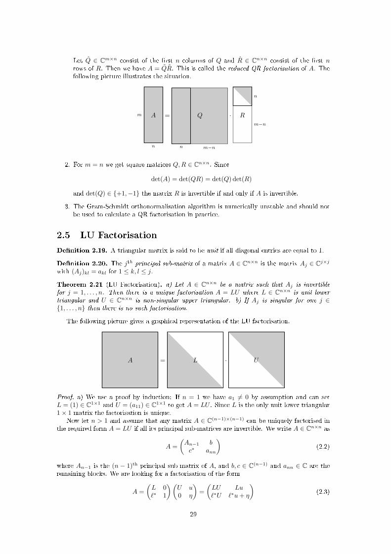
Let Q ∈ Cm×n consist of the rst n columns of Q and R ∈ Cn×n consist of the rst nrows of R. Then we have A = QR. This is called the reduced QR factorisation of A. Thefollowing picture illustrates the situation.
Am
n
= Q
n m−n
· R
n
m−n
2. For m = n we get square matrices Q,R ∈ Cn×n. Since
det(A) = det(QR) = det(Q) det(R)
and det(Q) ∈ +1,−1 the matrix R is invertible if and only if A is invertible.
3. The Gram-Schmidt orthonormalisation algorithm is numerically unstable and should notbe used to calculate a QR factorisation in practice.
2.5 LU Factorisation
Denition 2.19. A triangular matrix is said to be unit if all diagonal entries are equal to 1.
Denition 2.20. The jth principal sub-matrix of a matrix A ∈ Cn×n is the matrix Aj ∈ Cj×jwith (Aj)kl = akl for 1 ≤ k, l ≤ j.
Theorem 2.21 (LU Factorisation). a) Let A ∈ Cn×n be a matrix such that Aj is invertiblefor j = 1, . . . , n. Then there is a unique factorisation A = LU where L ∈ Cn×n is unit lowertriangular and U ∈ Cn×n is non-singular upper triangular. b) If Aj is singular for one j ∈1, . . . , n then there is no such factorisation.
The following picture gives a graphical representation of the LU factorisation.
A = L · U
Proof. a) We use a proof by induction: If n = 1 we have a1 6= 0 by assumption and can setL = (1) ∈ C1×1 and U = (a11) ∈ C1×1 to get A = LU . Since L is the only unit lower triangular1× 1-matrix the factorisation is unique.
Now let n > 1 and assume that any matrix A ∈ C(n−1)×(n−1) can be uniquely factorised inthe required form A = LU if all its principal sub-matrices are invertible. We write A ∈ Cn×n as
A =(An−1 bc∗ ann
)(2.2)
where An−1 is the (n − 1)th principal sub-matrix of A, and b, c ∈ C(n−1) and ann ∈ C are theremaining blocks. We are looking for a factorisation of the form
A =(L 0`∗ 1
)(U u0 η
)=(LU Lu`∗U `∗u+ η
)(2.3)
29
with L ∈ C(n−1)×(n−1) unit lower triangular, U ∈ C(n−1)×(n−1) invertible upper triangular,`, u ∈ Cn−1 and η ∈ C\0. We compare the blocks of (2.2) and (2.3).
By the induction hypothesis L and U with An−1 = LU exist and are unique. Since the matrixL is invertible the condition Lu = b determines a unique vector u. Since U is invertible there isan uniquely determined ` with U∗` = c and thus `∗U = c∗. Finally the condition `∗u+ η = annuniquely determines η ∈ C. This shows that the required factorisation for A exists and is unique.Since 0 6= det(A) = 1 · η · detU the upper triangular matrix is non-singular and η 6= 0.
b) Assume that A has an LU factorisation and let j ∈ 1, . . . , n. Then we can write A = LUin block form as(
A11 A12
A21 A22
)=(L11 0L21 L22
)(U11 U12
0 U22
)=(L11U11 L11U12
L21U11 L21U12 + L22U22
)where A11, L11, U11 ∈ Cj×j . We get
det(Aj) = det(A11) = det(L11U11) = det(L11) det(U11) = 1 · det(U11) 6= 0
and thus Aj is non-singular.
To illustrate the failure of LU factorisation when the principal submatrices are not invertible,consider the following matrix:
A =
0 0 11 1 00 2 1
This matrix is clearly non-singular: det(A) = 2. However, both principal sub-matrices aresingular:
A1 = (0)
A2 =(
0 01 1
)and therefore the factorisation A = LU is not possible. In contrast,
A′ =
1 1 00 2 10 0 1
(which is a permutation of the rows of A) has non-singular principal sub-matrices
A′1 = (1)
A′2 =(
1 10 2
)and hence A′ has an LU factorisation.
Because a non-singular matrix may not have an LU factorisation, while that same matrixwith its rows interchanged may be factorisable, it is of interest to study the eect of permutationson LU factorisation.
Theorem 2.22 (LU Factorisation with Permutations). If A ∈ Cn×n is invertible, then thereexists a permutation matrix P ∈ Cn×n, unit lower triangular L ∈ Cn×n, and non-singular uppertriangular U ∈ Cn×n such that PA = LU .
Proof. We prove the result by induction. Note that the base case n = 1 is straightforward:P = L = 1 and U = A 6= 0. Now assume the theorem is true for the (n− 1)× (n− 1) case. LetA ∈ Cn×n be invertible. Choose a permutation P1 such that
(P1A)11 := a 6= 0.
30
This is possible since A invertible implies that the rst column of A has a non-zero entry andP1 permutes rows. Now we can factorise P1A as follows:
P1A :=(a u∗
l B
)=(
1 0l/a I
)(a u∗
0 A
)
which is possible if A = B − lu∗/a = B − 1a l ⊗ u. Now
0 6= det(A) = ± det(P1A) = a det(A)
and so det(A) 6= 0 since a 6= 0. Thus A is invertible and A = P2LU . Hence
P1A =(
1 0l/a I
)(1 00 P2L
)(a u∗
0 U
)=(
1 0l/a P2L
)(a u∗
0 U
)=(
1 00 P2
)(1 0
PT2 l/a L
)(a u∗
0 U
)= P3LU ,
and thereforePT3 P1A = LU .
Note that L is unit lower triangular and that det(U) = adet(U) 6= 0 so that U is non-singularupper trangular. Since P = PT3 P1 is a permutation the result follows.
2.6 Cholesky Factorisation
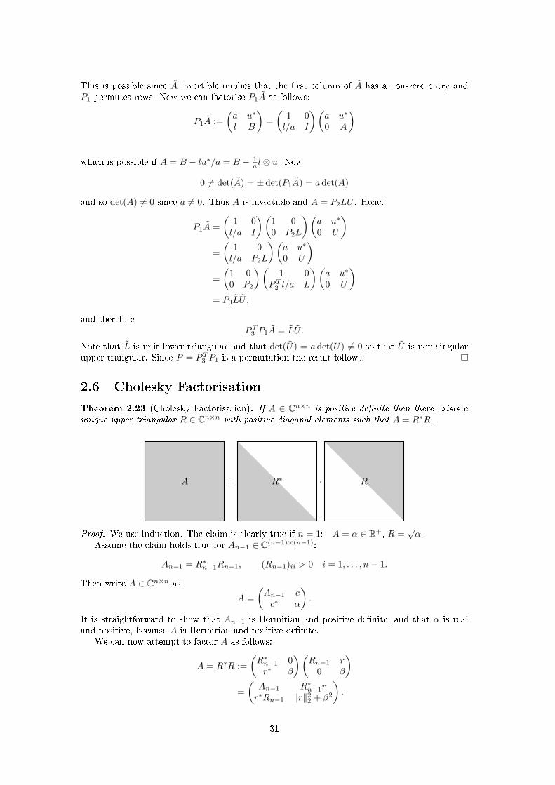
Theorem 2.23 (Cholesky Factorisation). If A ∈ Cn×n is positive denite then there exists aunique upper triangular R ∈ Cn×n with positive diagonal elements such that A = R∗R.
A = R∗ · R
Proof. We use induction. The claim is clearly true if n = 1: A = α ∈ R+, R =√α.
Assume the claim holds true for An−1 ∈ C(n−1)×(n−1):
An−1 = R∗n−1Rn−1, (Rn−1)ii > 0 i = 1, . . . , n− 1.
Then write A ∈ Cn×n as
A =(An−1 cc∗ α
).
It is straightforward to show that An−1 is Hermitian and positive denite, and that α is realand positive, because A is Hermitian and positive denite.
We can now attempt to factor A as follows:
A = R∗R :=(R∗n−1 0r∗ β
)(Rn−1 r
0 β
)=(An−1 R∗n−1rr∗Rn−1 ‖r‖22 + β2
).
31
For this factorisation to work we require r ∈ Cn−1 and β ∈ R+ such that
R∗n−1r = c
β2 = α− ‖r‖22.
Since Rn−1 is non-singular (positive diagonal elements), r and β are uniquely dened.It remains to show β ∈ R+. Note that, since A has positive eigenvalues det(A) > 0 and so
0 < det(A) = det(R∗R) = det(R∗) det(R)
= β2 det(R∗n−1) det(Rn−1 = β2 det(Rn−1)2.
Here we have used the fact that det(R∗n−1) = det(Rn−1) because Rn−1 is triangular with realpositive entries. But det(Rn−1)2 ∈ R+ since Rn−1 has diagonals in R+. Thus β2 > 0 and wecan choose β ∈ R+.
Bibliography
The books [Bha97], [HJ85] and [Ner71] all present matrix factorisations in a theoretical context.The books [Dem97], [GL96] and [TB97] all present related material, focussed on applications tocomputational algorithms. Theorem 2.7 is proved in [Ner71].
Exercises
Exercise 2-1. By following the proof of the existence of a singular value decomposition, ndan SVD for the following matrices:
A =(
1 23 1
), B =
−2 0 12 0 10√
18 0
.
Exercise 2-2. Show that a symmetric positive denite matrix A ∈ Rn×n can be written in theform
A =(a zT
z A1
)=(α 01αz I
)(1 00 A1 − 1
azzT
)(α 1
αzT
0 I
).
where α =√a. Based on this observation nd an alternative proof of Theorem 2.23, for the
Cholesky factorisation of real symmetric positive denite matrices.
Exercise 2-3. Let A ∈ Rm×n have singular values (σi | i = 1, . . . , n ). Show that ‖A‖2 = σmaxand, if m = n and A is invertible, ‖A−1‖−1
2 = σmin.
Exercise 2-4. Prove Theorem 1.16 concerning properties of similar matrices.
32
Chapter 3
Stability and Conditioning
Rounding errors lead to computational results which are dierent from the theoretical ones.The methods from this chapter will help us to answer the following question: how close is thecalculated result to the correct one?
It is common to view the computed solution of a problem in linear algebra as the exactsolution to a perturbed problem. This approach to the study of error is known as backwarderror analysis. If the perturbation is small (when measured in terms of machine precision)the algorithm is termed backward stable; when the perturbation is not small it is referred to asunstable. Thus the eect of computing the solution in oating point arithmetic, using a particularalgorithm, is converted into a perturbation of the original problem. Once this perturbed problemis known, the central issue in studying error is to estimate the dierence between the solutionof the original problem and a perturbed problem: the issue of conditioning. Conditioning is aproperty of the problem at hand, whilst the size of the perturbation arising in the backwarderror analysis framework is a property of the algorithm.
The three problems (SLE), (LSQ) and (EVP) can all be viewed as solving a linear or nonlinearequation of the form
G(y, η) = 0, (3.1)
for some G : Cp × Cq → Cp. Here y is the solution that we want to nd, and η the data whichdenes the problem. For (SLE) and (LSQ) the problem is linear and y = x (see below for aproof of this for (LSQ)) and for (EVP) it is nonlinear and y = (x, λ). The parameter η is thusdened by the matrix A and, for (SLE) and (LSQ), the matrix A and the vector b. Backwarderror analysis will enable us to show that the computed solution y solves
G(y, η) = 0.
Conditioning is concerned with estimating y− y in terms of η− η. Since conditioning of a givenproblem will aect the error analysis for all algorithms applied to it, we start with its study, foreach of our three problems in turn. The following denition will be useful in this chapter.
Denition 3.1. Let f = f(η) : Cq → Cp. We write f = O(‖η‖α) for α > 0 if there is a constantC > 0 such that ‖f‖ ≤ C‖η‖α uniformly as η → 0.
3.1 Conditioning of SLE
A problem is called well conditioned if small changes in the problem only lead to small changesin the solution and badly conditioned if small changes in the problem can lead to large changesin the solution. In this context the following denition is central.
Denition 3.2. The condition number κ(A) of a matrix A ∈ Cn×n in the norm ‖ · ‖ is thenumber
κ(A) =
‖A‖ · ‖A−1‖ if A is invertible and
+∞ else.
33
For this section x a vector norm ‖ · ‖ and an induced matrix norm ‖ · ‖. By Theorem 1.27these norms then satisfy
‖Ax‖ ≤ ‖A‖ · ‖x‖ for all x ∈ Cn, A ∈ Cn×n
‖I‖ = 1.
Remark. We always have ‖I‖ = ‖AA−1‖ ≤ ‖A‖‖A−1‖ = κ(A). For induced matrix norms thisimplies κ(A) ≥ 1 for every A ∈ Cn×n.
Example. Let A be real, symmetric and positive-denite with eigenvalues
λmax = λ1 ≥ λ2 ≥ · · · ≥ λn = λmin > 0.
Then we have ‖A‖2 = λmax. Since the matrix A−1 has eigenvalues 1/λ1, . . . , 1/λn we nd‖A−1‖2 = λ−1
minand thus the condition number of A in the 2-norm is
κ(A) =λmax
λmin
. (3.2)
Proposition 3.3. Let Ax = b and A(x+ ∆x) = b+ ∆b. Assume b 6= 0. Then
‖∆x‖‖x‖
≤ κ(A)‖∆b‖‖b‖
.
Proof. If A is not invertible the right hand side of the inequality is +∞ and the result holds.Thus we assume that A is invertible and we have
‖b‖ = ‖Ax‖ ≤ ‖A‖‖x‖. (3.3)
Since A−1∆b = ∆x we get
‖∆x‖‖x‖
=‖A−1∆b‖‖x‖
≤ ‖A−1‖‖∆b‖‖x‖
≤ ‖A‖‖A−1‖‖∆b‖‖b‖
where the last inequality is a consequence of (3.3).
The previous proposition gave an upper bound on how much the solution of the equationAx = b can change if the right hand side is perturbed. The result shows that the problem is wellconditioned if the condition number κ(A) is small. Proposition 3.5 below gives a similar resultfor perturbation of the matrix A instead of the vector b. For the proof we will need the followinglemma.
Lemma 3.4. Assume that A ∈ Cn×n satises ‖A‖ < 1 in some induced matrix norm. ThenI +A is invertible and
‖(I +A)−1‖ ≤ (1− ‖A‖)−1.
Proof. With the triangle inequality we get
‖x‖ = ‖(I +A)x−Ax‖≤ ‖(I +A)x‖+ ‖ −Ax‖≤ ‖(I +A)x‖+ ‖A‖‖x‖
and thus‖(I +A)x‖ ≥
(1− ‖A‖
)‖x‖
for every x ∈ Cn. Since this implies (I +A)x 6= 0 for every x 6= 0, and thus the matrix I +A isinvertible.
Now let b 6= 0 and x = (I +A)−1b. Then
‖(I +A)−1b‖‖b‖
=‖x‖
‖(I +A)x‖≤ 1
1− ‖A‖.
34
Since this is true for all b 6= 0, we have
‖(I +A)−1‖ = supb 6=0
‖(I +A)−1b‖‖b‖
≤ 11− ‖A‖
.
This completes the proof.
Proposition 3.5 (Conditioning of SLE). Let x solve the equations
Ax = b and (A+ ∆A)(x+ ∆x) = b.
Assume that A is invertible with condition number κ(A) in some induced matrix norm ‖ · ‖.Then we have, for κ(A)‖∆A‖ < ‖A‖,
‖∆x‖‖x‖
≤ κ(A)
1− κ(A)‖∆A‖‖A‖
· ‖∆A‖‖A‖
.
Proof. Note that
‖A−1∆A‖ ≤ ‖A−1‖‖∆A‖ = κ(A)‖∆A‖‖A‖
< 1. (3.4)
Here I +A−1∆A is invertible by Lemma 3.4.We have
(A+ ∆A)∆x = −∆Ax
and thus(I +A−1∆A)∆x = −A−1∆Ax.
Using Lemma 3.4 we can write
∆x = −(I +A−1∆A)−1A−1∆Ax
and we get
‖∆x‖ ≤ ‖(I +A−1∆A)−1‖‖A−1∆A‖‖x‖ ≤ ‖A−1∆A‖1− ‖A−1∆A‖
‖x‖.
Using (3.4) and the fact that the map x 7→ x/(1 − x) is increasing on the interval [0, 1) weget
‖∆x‖‖x‖
≤κ(A)‖∆A‖‖A‖
1− κ(A)‖∆A‖‖A‖
.
This is the required result.
Refer to Exercise 3-2 for a result which combines the statements of propositions 3.3 and 3.5.
3.2 Conditioning of LSQ
In this section we study the conditioning of the following problem: given A ∈ Cm×n with m ≥ n,rank(A) = n and b ∈ Cm, nd x ∈ Cn which minimizes ‖Ax− b‖2.
For expository purposes consider the case where A and b are real. Notice that then x solving(LSQ) minimizes ϕ : Rn → R given by
ϕ(x) :=12〈Ax,Ax〉 − 〈Ax, b〉+
12‖b‖22.
This is equivalent to minimizing
12〈x,A∗Ax〉 − 〈x,A∗b〉+
12‖b‖22.
35
(Note that A∗ = AT in this real case). This quadratic form is positive-denite since A∗A isHermitian and has positive eigenvalues under (3.5). The quadratic form is minimized where thegradient is zero, namely where
A∗Ax = A∗b.
Although we have derived this in the case of real A, b, the nal result holds as stated in thecomplex case; see Chapter 7.
Consider the reduced SVD A = U ΣV ∗ where U ∈ Cm×n, Σ ∈ Rn×n with Σii = σi, andV ∈ Cn×n. The assumption on rank(A) implies, by Theorem 2.15,
σ1 ≥ σ2 ≥ · · · ≥ σn > 0. (3.5)
In particular, A∗A = V Σ2V ∗ is invertible. The solution of (LSQ) is hence unique and given bysolution of the normal equations
x = (A∗A)−1A∗b.
Denition 3.6. For A ∈ Cm×n, the matrix A† = (A∗A)−1A∗ ∈ Cn×m is called the pseudo-inverse (or Moore-Penrose inverse) of A.
With this notation the solution of (LSQ) is
x = A†b.
Denition 3.7. For A ∈ Cm×n with m ≥ n and n positive singular values, dene the conditionnumber of A in the norm ‖ · ‖ to be
κ(A) =
‖A‖ · ‖A†‖ if rank(A) = n and
+∞ else.
Remark. Since for square, invertible matrices A we have A† = A−1, the denition of κ(A) isconsistent with the previous one for square matrices. As before the condition number dependson the chosen matrix norm.
Lemma 3.8. Let A ∈ Cm×n with m ≥ n have n positive singular values satisfying (3.5). Thenthe condition number in the ‖ · ‖2-norm is
κ(A) =σ1
σn.
Proof. Let A = U ΣV ∗ be a reduced SVD of A. Then A∗A = V Σ2V ∗ and thus
A† = V Σ−1U∗. (3.6)
This equation is a reduced SVD for A† (modulo ordering of the singular values) and it can beextended to a full SVD by adding m−n orthogonal columns to U and zeros to Σ−1. Doing thiswe nd, by Corollary 2.13,
κ(A) = ‖A‖2‖A†‖2 = σ1 ·1σn.
Notice that (3.6) impliesAx = AA†b = U U∗b
and hence that‖Ax‖2 ≤ ‖UU∗b‖2 = ‖U∗b‖2 = ‖b‖2
by the properties of orthogonal matrices. Thus we may dene θ ∈ [0, π/2] by cos(θ) = ‖Ax‖2‖b‖2 .
36
Theorem 3.9. Assume that x solves (LSQ) for (A, b) and x+ ∆x solves (LSQ) for (A, b+ ∆b).Dene η = ‖A‖2‖x‖2/‖Ax‖2 ≥ 1. Then we have
‖∆x‖2‖x‖2
≤ κ(A)η cos(θ)
· ‖∆b‖2‖b‖2
where κ(A) is the condition number of A in ‖ · ‖2-norm.
Proof. We have x = A†b and x+ ∆x = A†(b+ ∆b). Linearity then gives ∆x = A†∆b and we get
‖∆x‖2‖x‖2
≤ ‖A†‖2‖∆b‖2‖x‖2
=κ(A)‖∆b‖2‖A‖2‖x‖2
=κ(A)‖∆b‖2η‖Ax‖2
=κ(A)η cos(θ)
· ‖∆b‖2‖b‖2
.
Remark. The constant κ(A)/η cos(θ) becomes large if either κ(A) is large or θ ≈ π/2. In eitherof these cases the problem is badly conditioned. The rst case involves only the singular valuesof A. The second case involves a relationship between A and b. In particular cos(θ) is small ifthe range of A is nearly orthogonal to b. Then
ϕ(x) ≈ 12‖Ax‖22 +
12‖b‖22
so that simply setting x = 0 gives a good approximation to the minimizer; in this case smallchanges in b can induce large relative changes in x.
Proof of the following result is left as Exercise 3-4.
Theorem 3.10. Let θ and η as above. Assume that x solves (LSQ) for (A, b) and x+∆x solves(LSQ) for (A+ ∆A, b). Then
‖∆x‖2‖x‖2
≤(κ(A) +
κ(A)2 tan(θ)η
)· ‖∆A‖2‖A‖2
where κ(A) is the condition number of A in ‖ · ‖2-norm.
More generally, when both the matrix A and vector b are perturbed one has
Theorem 3.11 (Conditioning of LSQ). Assume that x solves (LSQ) for (A, b) and x + ∆xsolves (LSQ) for (A+ ∆A, b+ ∆b). Let r = b−Ax and
δ = max(‖∆A‖2‖A‖2
,‖∆b‖2‖b‖2
).
Then‖∆x‖2‖x‖2
≤ κ(A)δ1− κ(A)δ
(2 + (κ(A) + 1)
‖r‖2cos(θ)η‖b‖2
)where κ(A) is the condition number of A in ‖ · ‖2-norm.
3.3 Conditioning of EVP
In this section we will discuss the conditioning of the eigenvalue problem (EVP), i.e. we willdiscuss how much the eigenvalues of a matrix can change, if the matrix is changed by a smallamount. A preliminiary result is given in the following theorem: the eigenvalues change con-tinuously when the matrix is changed. A more detailed analysis is presented in the rest of thesection.
37
Theorem 3.12 (Continuity of Eigenvalues). Let λ(A) denote the vector of eigenvalues of thematrix A ∈ Cn×n, ordered in decreasing absolute value, and repeated according to algebraicmultiplicities. Then λ : Cn×n → Cn is continuous.
Proof. This follows since the eigenvalues are the roots of the characteristic polynomial of A; thishas coecients continuous in A.
Before discussing the conditioning of eigenvalue problems we make a brief diversion to statea version of the implicit function theorem (IFT) which we will then use.
Theorem 3.13 (IFT). Let G : Cl × Cm → Cm be two times dierentiable and assume thatG(x, y) = 0 for some (x, y) ∈ Cl × Cm. If DyG(x, y) is invertible then, for all suciently small∆x, there is a unique solution ∆y of the equation
G(x+ ∆x, y + ∆y) = 0
in a small ball at the origin. Furthermore the solution ∆y satises
DxG(x, y) ∆x+DyG(x, y) ∆y = O(‖∆x‖2
).
Denition 3.14. For A ∈ Cn×n, the eigenvalue condition number for an eigenvalue λ ∈ C of amatrix A ∈ Cn×n is
κA(λ) =
|〈x, y〉|−1, if 〈x, y〉 6= 0 and
∞, else,
where x and y are the normalised right and left eigenvectors for eigenvalue λ.
Theorem 3.15 (Conditioning of EVP). Let λ be a simple eigenvalue of A corresponding to rightand left normalized eigenvectors x and y. Assume 〈y, x〉 6= 0. Then for all suciently small∆A ∈ Cn×n the matrix A+ ∆A has an eigenvalue λ+ ∆λ with
∆λ =1〈y, x〉
(〈y,∆Ax〉+O
(‖∆A‖22
)).
Proof. Dene G : Cn×n × Cn × C→ Cn × C by
G(A, x, λ) =(Ax− λx
12‖x‖
22 − 1
2
).
Thus we have G(A, x, λ) = 0 if and only if x is a normalized eigenvector of A with eigenvalue λand clearly G ∈ C∞.
We will apply the IFT with l = n2 and m = n+1 to write (x, λ) as a function of A: Providedthe invertibility condition holds, the equation
G(A+ ∆A, x+ ∆x, λ+ ∆λ) = 0
has, for suciently small ∆A, a solution (∆x,∆λ) satisfying
DAG(A, x, λ) ∆A+D(x,λ)G(A, x, λ)(
∆x∆λ
)= O
(‖∆A‖2
).
Now computing the derivatives of G gives
D(x,λ)G(A, x, λ) =(A− λI −xx∗ 0
)∈ C(n+1)×(n+1)
and, for every C ∈ Cn×n,
DAG(A, x, λ) C =(Cx0
)∈ Cn+1
38

To show that D(x,λ)G(A, x, λ) is invertible assume D(x,λ)G(A, x, λ) (y, µ) = 0 for y ∈ Cn andµ ∈ C. It suces to show that this implies (y, µ) = 0. From
(A− λI)y − xµ = 0x∗y = 0
we get(A− λI)2y = 0 and 〈x, y〉 = 0.
This implies (A−λI) has a two dimensional null-space, contradicting simplicity by Lemma 1.17,unless y = 0. Hence it follows that y = 0, µ = 0, and so D(x,λ)G is invertible.
Finally, (∆δ
)=(
∆Ax0
)+(A− λI −xx∗ 0
)(∆x∆λ
).
satises‖∆‖2 + |δ| = O
(‖∆A‖22
).
by Theorem 3.13. Using∆ = ∆Ax+ (A− λI)∆x− x∆λ.
we nd−y∗x∆λ+ y∗∆Ax = y∗∆ = O
(‖∆A‖22
)and the result follows.
Corollary 3.16. Let λ be a simple eigenvalue of A corresponding to right and left normalizedeigenvectors x and y. Then for all suciently small ∆A ∈ Cn×n the matrix A + ∆A has aneigenvalue λ+ ∆λ with
|∆λ| ≤ κA(λ)(‖∆A‖2 +O
(‖∆A‖22
)).
3.4 Stability of Algorithms
The stability of an algorithm measures how susceptible the result is to rounding errors occurringduring the computation. Consider the general framework for all our problems, namely equation(3.1), where y denotes the solution we wish to compute and η the input data. Then we mayview a locally unique family of solutions to the problem as a mapping from the input data tothe solution: y = g(η). For example, for (SLE) we have y = x, η = (A, b) and g(η) = A−1b. Weassume that the algorithm returns the computed result y 6= y which can be represented as theexact image y = g(η) of a dierent input value η.
Denition 3.17. The quantity ∆y = y−y is called the forward error and ∆η = η−η is called abackward error. If η is not uniquely dened then we make the choice of η which results in minimal‖∆η‖. The relative backward error is ‖∆η‖/‖η‖ and the relative forward error is ‖∆y‖/‖y‖.
input data
results
η
η
y
y
exact
exact
computed∆η ∆y
39
As an illustration of the concept, imagine that we solve (SLE) and nd x satisfying Ax− b =∆b. Then ∆x := x− x is the forward error and ∆b the backward error. The following theoremis a direct consequence of Proposition 3.3.
Theorem 3.18. For the problem (SLE) we have
rel. forward error ≤ κ(A) · rel. backward error.
Internally computers represent real number using only a nite number of bits. Thus theycan only represent nitely many numbers and when dealing with general real numbers roundingerrors will occur. Let F ⊂ R be the set of representable numbers and let fl: R → F be therounding to the closest element of F.
In this book we will use a simplied model for computer arithmetic which is described by thefollowing two assumptions. The main simplication is that we ignore the problems of numberswhich are unrepresentable because they are very large (overows) or very close to zero (under-ows). We simply use a model in which every bounded interval of R is approximated by a niteset of numbers from F in such a way that the following assumption holds:
Assumption 3.19. There is a parameter εm > 0 (machine epsilon) such that the followingconditions hold.
A1: For all x ∈ R there is an ε ∈ (−εm,+εm) with
fl(x) = x · (1 + ε).
A2: For each operation ∗ ∈ +,−, ·, / and every x, y ∈ F there is a δ ∈ (−εm,+εm) with
x~ y = (x ∗ y) · (1 + δ)
where ~ denotes the computed version of ∗.
Denition 3.20. An algorithm, is called backward stable if the relative backward error satises
‖∆η‖‖η‖
= O(εm).
Remark. Some algorithms which are backward stable by the denition are termed unstable inpractice. This occurs when the constant in the O(εm) term depends badly on some measure ofthe problem dimension for instance grows exponentially in n for the (SLE). For this reason,rather than just stating a backward stability result, we will often try to identify a norm ‖ · ‖ andconstant C(n) such that
‖∆η‖‖η‖
≤ C(n)εm.
This, of course, establishes backward stability. But it gives more detailed information on exactlywhen the backward error is small, as a function of problem size. Note, however, that statementsabout the dependence of the constants in the backward error are norm-dependent. The denitionof backward stable itself is not.
The typical way to use backward stability is in a two-step procedure as follows. In the rststep, backward error analysis, one shows that the algorithm in question is backward stable, i.e.that the inuence of rounding errors can be represented as a small perturbation ∆x of the originalproblem. (This is a property of the algorithm used.) In the second step one uses results likeTheorem 3.18 about the conditioning of the problem (which does not depend on the algorithmused) to show that the forward error is also small. Together these steps show that the calculatedresult is close the the exact result.
We give a simple example of a backward stability calculation.
Lemma 3.21. The calculated subtraction is backward stable.
40
Proof. The exact result of a subtraction is given by g(x1, x2) = x1 − x2, the computed result isg(x1, x2) = fl(x1) fl(x2). Using Assumption A1 we get
fl(x1) = x1(1 + ε1) and fl(x2) = x2(1 + ε2)
with |ε1|, |ε2| < εm. Using Assumption A2 we get
fl(x1) fl(x2) =(fl(x1)− fl(x2)
)(1 + ε3)
where |ε3| < εm. This gives
fl(x1) fl(x2) =(x1(1 + ε1)− x2(1 + ε2)
)(1 + ε3)
= x1(1 + ε1)(1 + ε3)− x2(1 + ε2)(1 + ε3)= x1(1 + ε4)− x2(1 + ε5)
where ε4 = ε1 + ε3 + ε1ε3 and ε5 = ε2 + ε3 + ε2ε3 satisfy |ε4|, |ε5| ≤ 2εm +O(ε2m) = O(εm) for
εm → 0.Thus for the input error we can choose
x =(x1
x2
), x =
(x1(1 + ε4)x2(1 + ε5)
), ∆x = x− x
and we get ‖∆x‖2 =√ε2
4x21 + ε2
5x22 ≤ O(εm)‖x‖2. This completes the proof.
Remarks.
1. The above proof is a case where the x from the denition of the backward error is notuniquely determined. But since we are only interested in the x which minimizes thebackward error, we can choose any x which gives the result ‖∆x‖2 ≤ O(εm)‖x‖2. Theoptimal x can only be better.
2. Similar proofs show that the operations ⊕, and are also backward stable.
3. Proofs of backward stability have to analyse the inuence of rounding errors and thus aretypically based on our Assumptions A1 and A2 about computer arithmetic. Since theytend to be long and involved we omit most of these proofs in this book. We frequentlystudy the statements of backward stability results, however, as they give useful practicalinsight into the ecacy of algorithms.
Bibliography
Conditioning for the basic problems of numerical linear algebra is a central part of the pre-sentation in [Dem97]. Numerical stability is introduced, and thoroughly studied, in a range ofcontexts arising in numerical linear algebra, in [Hig02]. Theorem 3.10 may be found in [Dem97]and Theorem 3.11 in [Hig02]. The Implicit Function Theorem 3.13 is proved in [CH96].
Exercises
Exercise 3-1. Choose a matrix norm and calculate the condition number of the matrix
A =(ε 11 1
)in this norm.
Exercise 3-2. Assume that A is invertible with κ(A)‖∆A‖/‖A‖ < 1 in some induced matrixnorm. Let x be a solution of Ax = b and let x be a solution of (A+ ∆A)x = b+ ∆b. Show that
‖x− x‖‖x‖
≤ κ(A)
1− κ(A)‖∆A‖‖A‖
·(‖∆A‖‖A‖
+‖∆b‖‖b‖
).
41

Exercise 3-3. Let A = UΣV T be an SVD factorization of A ∈ Rm×n with m ≥ n and rank=n.Prove that there exists a matrix ∆A with ‖∆A‖2 = σmin such that A + ∆A does not haverank n.
Exercise 3-4. Prove Theorem 3.10.
Exercise 3-5. Show that the calculated arithmetic operations ⊕, and are backward stable.
42
Chapter 4
Complexity of Algorithms
In this chapter we study methods which quantify how long it takes to solve a numerical problemon a computer. Specically we focus on the question how the run time, as measured by thenumber of algebraic operations, depends on some measure of the problem size.
4.1 Computational Cost
The computational cost of an algorithm is the amount of resources it takes to perform this algo-rithm on a computer. For simplicity here we just count the number of oating point operations(additions, subtractions, multiplications, divisions) performed during one run of the algorithm,together with a count of the number of square roots taken; on one occasion we also count thenumber of comparisons between real numbers. A more detailed analysis would also take factorslike memory usage into account.
Denition 4.1. The cost of an algorithm is
C(n) = number of additions, subtractions, multiplications, divisions and square roots
where n is the size of the input data (e.g. the number of equations etc.).
The following denition provides the notation we will use to describe the asyptotic compu-tation cost of an algorithm, this is the behaviour of the cost C(n) for n → ∞. (In the case ofthe notation O it is closely related to the notation used in Denition 3.1 from the last chapter,except that there we consider the order of magnitude of small quantities. Here our concern withcost leads to consideration of the order of magnitude of large quantities. However, the denitionsbelow can be adapted to the case x→ 0 and we will sometimes use this without comment.)
Denition 4.2. For f, g : N→ N or f, g : R+ → R+ we write
g(x) = O(f(x)
)if lim sup
x→∞
g(x)f(x)
<∞,
g(x) = Ω(f(x)
)if lim inf
x→∞
g(x)f(x)
> 0,
g(x) = Θ(f(x)
)if g(x) = Ω(f(x)) and g(x) = O(f(x)),
g(x) ∼ f(x) if limx→∞
g(x)f(x)
= 1.
Example. From the denition we can see that the property g(x) ∼ f(x) implies g(x) = Θ(f(x)
).
Example. Using this notation we can write 5n2 + 2n − 3 ∼ 5n2 = Θ(n2), n2 = O(n3) andn2 = Ω(n).
43
Algorithm (standard inner product algorithm).input: x, y ∈ Cnoutput: s = 〈x, y〉1: s = x1y1
2: for i = 2, . . . , n do3: s = s+ xiyi4: end for5: return s
Theorem 4.3. The standard inner-product algorithm on Cn has computational cost C(n) =Θ(n). Any algorithm for the inner product has C(n) = Ω(n).
Proof. The standard inner-product algorithm above has n multiplications and n − 1 additions,i.e. C(n) = 2n− 1 = Θ(n). Sketch of the proof for C(n) = Ω(n): since each of the products xiyiis independent of the others, we have to calculate all n of them.
Remark. Giving a real proof for the lower bound in the above theorem would require a detailedmodel about what an algorithm actually is. One would for example need to be able to work ina framework where guessing the result in just one operation and returning it is not a properalgorithm. We avoid these diculties here by only giving sketches for lower bounds.
Algorithm (standard matrix-vector multiplication).input: A ∈ Cm×n, x ∈ Cnoutput: y = Ax ∈ Cmlet a∗1, . . . , a
∗m denote the rows of A.
1: for i = 1, . . . ,m do2: let yi = 〈ai, x〉 using the standard inner product algorithm3: end for4: return y
Theorem 4.4. The computational complexity of the standard method for Cn×n-matrix-vectormultiplication satises C(n) = Θ(n2). Any method has C(n) = Ω(n).
Proof. See Exercise 4-2.
Algorithm (standard matrix-matrix multiplication).input: A ∈ Cl×m with rows a∗1, . . . , a
∗l , B ∈ Cm×n with columns b1, . . . , bn
output: C = AB ∈ Cl×n
1: for i = 1, . . . , l do2: for j = 1, . . . , n do3: let cij = 〈ai, bj〉 using the standard inner product algorithm4: end for5: end for6: return C
Theorem 4.5. The standard method for Cn×n-matrix-matrix multiplication satises C(n) =Θ(n3). Any method has C(n) = Ω(n2).
Proof. We have to calculate n2 inner products. Thus the asymptotic computational cost isC(n) = n2Θ(n) = Θ(n3). Sketch for the lower bound: we have to calculate n2 entries of theresulting matrix and thus C(n) ≥ n2.
44
4.2 Matrix-Matrix Multiplication
In Theorem 4.5 there is a gap between the order Θ(n3) of the standard method for multiplyingmatrices and the lower bound Ω(n2). The purpose of this section is to show that there areactually algorithms with an asymptotic order which is better than Θ(n3).
For A,B ∈ Cn×n, n even and D = AB write
A =(A11 A12
A21 A22
), B =
(B11 B12
B21 B22
), D =
(D11 D12
D21 D22
)where Aij , Bij , Dij ∈ Cn/2×n/2. Then we have
D11 = A11B11 +A12B21
D12 = A11B12 +A12B22
D21 = A21B11 +A22B21
D22 = A21B12 +A22B22.
The above method calculates the product of two n × n-matrices using eight multiplicationsof (n/2) × (n/2)-matrices. Using this idea recursively leads to an algorithm for n × n matrixmultplication which builds the answer from the multplication of small matrices. The cost thensatises
C(n) = 8C(n/2) + n2
with the n2 contribution coming from the 4 additions of (n/2) × (n/2) matrices. Exercise 4-4shows that this leads to a cost of Θ(n3) and is thus no better than the standard algorithm.
There is, however, another way to calculate the entries of the matrix D, which is algebraicallymore complicated, but, crucially, only uses seven multiplications of (n/2) × (n/2)-matrices. Itwill transpire that this fact can be utilised to get an asymptotically faster method of multiplyingmatrices. Using
P1 = (A11 +A22)(B11 +B22)P2 = (A21 +A22)B11
P3 = A11(B12 −B22)P4 = A22(B21 −B11)P5 = (A11 +A12)B22
P6 = (A21 −A11)(B11 +B12)P7 = (A12 −A22)(B21 +B22)
we can write
D11 = P1 + P4 − P5 + P7
D12 = P3 + P5
D21 = P2 + P4
D22 = P1 + P3 − P2 + P6.
Algorithm (Strassen Multiplication).input: A,B ∈ Cn×n with n = 2k for some k ∈ N0
output: D = AB ∈ Cn×n
1: if n = 1 then2: return AB3: else4: calculate P1, . . . , P7 (using recursion)5: calculate D11, D12, D21 and D22
6: return D7: end if
45
Remark. Recursive algorithms of this kind are called divide and conquer algorithms.
Using the Strassen-multiplication we can calculate D with 7 multiplications of n2 ×n2 -matrices
and 18 additions of n2 ×n2 -matrices. Thus we nd
C(n) = 7C(n/2) + 18n2/4.
Lemma 4.6. The Strassen-multiplication has computational cost C(2k) = 7 · 7k − 6 · 4k for allk ∈ N0.
Proof. For k = 0 we get C(20) = C(1) = 1.Assume the claim is true for k ∈ N0. Then
C(2k+1) = 7C(2k) + 18 (2k)2
= 7(7 · 7k − 6 · 4k) + 18 · 4k
= 7 · 7k+1 − (7 · 6− 18)4k
= 7 · 7k+1 − 6 · 4k+1.
Now the claim follows by induction.
Theorem 4.7 (Strassen Multiplication). Using the Strassen-algorithm it is possible to con-struct an algorithm for matrix-matrix multiplication with asymptotic computational cost C(n) =Θ(nlog2 7).
Proof. We rst prove the theorem for n = 2k, k ∈ N0. Then we have
7k = 2log2(7k) = 2k log2 7 = (2k)log2 7 = nlog2 7
and4k = (2k)2 = n2.
Using the lemma we get
C(n) = 7 · 7k − 6 · 4k = 7nlog2 7 − 6 · n2 = Θ(nlog2 7).
This nishes the proof.If n is not a power of 2 then we argue as follows. We can extend the matrices: choose k ∈ N0
with 2k ≥ n > 2k−1 and dene A, B ∈ C2k×2k
by
A =(A 012
021 022
), B =
(B 012
021 022
)where 012 ∈ Cn×(2k−n), 021 ∈ C(2k−n)×n and 022 ∈ C(2k−n)×(2k−n) are zero-matrices of appro-priate size. The product of A and B may again be written in block form:
AB =(AB 012
021 022
)Thus we can nd the product of the n×n-matrices A and B by multiplying the 2k×2k-matricesA and B with the Strassen-algorithm. Since we have n ≤ 2k ≤ 2n, the extended matrices are atmost double the size of the original ones, and because (2n)α = Θ(nα) for every α > 0 the resultfor n = 2k implies C(n) = Θ(nlog2 7) as required.
Remark. By ideas similar to (but more involved than) those used by Strassen it is possible toconstruct an algorithm which multiplies matrices in O(n2.376...). It remains an open questionwhether the exponent can be made arbitrarily close to 2.
46
Often the rst method encountered for matrix inversion is Cramer's rule:
A−1 =adj(A)det(A)
.
Using the naive way to calculate det(A) takes Θ(n!) operations, and so for Cramer's rule wewould get asymptotic computational cost
C(n) = Θ(n!) = Θ(e−n/2nn).
Although of theoretical importance, this is a totally inecient method to invert a matrix. Thenext result indicates why.
Theorem 4.8 (Complexity of Matrix Inversion). If there is a method to multiply n×n-matriceswith asymptotic computational cost O(nα) for some α ≥ 2, then it is also possible to invertn× n-matrices with cost O(nα).
Proof. Let A ∈ Cn×n be invertible. The proof consists of three steps.1) As in the previous theorem we can restrict ourselves to the case n = 2k for some k ∈ N0.
If n is not of this form we extend the matrix: choose k ∈ N0 with 2k ≥ n > 2k−1 and dene thematrix A ∈ C2k×2k
by
A =(A 012
021 I22
)where 012 ∈ Cn×(2k−n) and 021 ∈ C(2k−n)×n are zero-matrices and I22 is the (2k−n)× (2k−n)-identity matrix. Then the inverse of this matrix is
A−1 =(A−1 012
021 I22
)and we can invert A by inverting the 2k×2k-matrix A. Since Θ
((2n)α
)= Θ
(nα)the asymptotic
cost is unchanged.2) Since A is invertible we have
x∗(A∗A)x = (Ax)∗Ax = ‖Ax‖22 > 0
for every x 6= 0 and thus A∗A is positive denite and therefore invertible. We can write
A−1 = (A∗A)−1A∗.
This allows us to invert A with cost C(n) = D(n) + O(nα) where D is the cost of inverting aHermitian, positive denite matrix and O(nα) is the cost for matrix-matrix multiplication. Sowe can restrict ourselves to the case of Hermitian, positive denite matrices.
3) To determine the cost function D let B be Hermitian and positive denite:
B =(B11 B12
B∗12 B22
)where the Bjk are
n2 ×
n2 -matrices. Let S = B22−B∗12B
−111 B12, known as the Schur complement.
A direct calculation shows that
B−1 =(B−1
11 +B−111 B12S
−1B∗12B−111 −B−1
11 B12S−1
−S−1B∗12B−111 S−1
).
From exercise 4-3 we know that the matrices B11 and S are invertible.This method to calculate B−1 needs 2 inversions of n
2 ×n2 -matrices (namely of B11 and of
S), a products of n2 ×n2 -matrices and b sums/subtractions of n2 ×
n2 -matrices where a and b are
independent of n. This shows that
D(n) ≤ 2D(n/2) +O(nα) +O(n2)
47
where O(nα) is the cost for the multiplications and O(n2) is the cost for the additions andsubtractions.
From Theorem 4.5 we already know α ≥ 2, so we can simplify the above estimate to
D(n) ≤ 2D(n/2) + cnα
for some constant c > 0. With an induction argument (see Exercise 4-5 below) one can conclude
D(2k) ≤ c
1− 21−α (2k)α
and thus we getD(2k) = O
((2k)α
)for k →∞. This nishes the proof.
4.3 Fast Fourier Transform
The previous section shows that the inner-product based algorithm for matrix-matrix multipli-cation can be substantially improved by use of a recursive divide and conquer approach. We nowattempt a similar improvement of matrix-vector multiplication, over the inner-product based al-gorithm. However, in contrast to the matrix-matrix case, the idea we present here works only fora restricted class of matrices the discrete Fourier transform matrices. However other, similar,ideas have also been developed for other discrete transforms. The technique we present here isprototypical of a whole range of results available for matrix-vector multiplications of structuredmatrices.
As an abbreviation writeωn = e2πi/n
and dene the vectors ϕl ∈ Cn for l = 0, . . . , n− 1 by
ϕl =1√n
((e−2πil/n)0, (e−2πil/n)1, . . . , (e−2πil/n)n−1
)=
1√n
(1, ω−ln , ω−2l
n , . . . , ω−(n−1)ln
).
The following lemma shows that these vectors form a basis of Cn.
Lemma 4.9. 〈ϕl, ϕm〉 = δlm.
Proof.
〈ϕl, ϕm〉 =1n
n−1∑j=0
ω(l−m)jn .
If l = m, clearly 〈ϕl, ϕm〉 = 1. If l 6= m the geometric sum gives
1n
ω(l−m)nn − 1
ω(l−m)n − 1
.
But ω(l−m)nn = e2πi(l−m) = 1 implying 〈ϕl, ϕn〉 = 0.
Hence the ϕln−1l=0 form an orthonormal basis for Cn. Thus any vector u ∈ Cn can be
expanded as
u =n−1∑l=0
alϕl,
where u, ϕl ∈ Cn and the al ∈ C.
48
The al can be found using orthogonality:
〈ϕm, u〉 =n−1∑l=0
al〈ϕm, ϕl〉 =n−1∑l=0
alδml = am.
Thus am = 〈ϕm, u〉.Writing this out, with ωn denoted by ω for simplicity, gives
a0
a1
...
...an−1
=1√n
1 1 1 . . . 11 ω ω2 . . . ωn−1
1 ω2 ω4 . . . ω2(n−1)
.... . .
1 ωn−1 ω2(n−1) . . . ω(n−1)2
︸ ︷︷ ︸
:=An
u .
Thus to expand arbitrary u in the basis ϕk we need to be able to perform matrix vectormultiplication by An ∈ Cn×n.
Theorem 4.10 (Complexity of FFT Matrix-Vector Multiply). Let n = 2k. Matrix-vector mul-tiplication by An ∈ Cn×n can be performed in O(n log n) time.
Proof. We letFk =
√nAn with n = 2k.
Note that Fk−1 ∈ Cn/2×n/2 and is built from ωn/2. We prove that multiplication by Fk can be
eected in O(k2k) time, which gives the desired result.Let
x = (x0, x1, . . . , xn−1)T ∈ C2k
xe = (x0, x2, . . . , xn−2)T ∈ C2k−1
xo = (x1, x3, . . . , xn−1)T ∈ C2k−1.
Knowledge of xo, xe gives x. Let
y = Fkx, y∗ = ((yt)∗, (yb)∗)∗.
Then, for j = 0, . . . , 2k − 1,
yj =2k−1∑l=0
ωjl2kxl
=2k−1−1∑l=0
ω2jl2k x2l +
2k−1−1∑l=0
ωj(2l+1)
2k x2l+1.
But ω2jl2k = e2πi(2jl)/2k
= e2πi(jl)/2k−1= ωjl
2k−1 , and so ωj(2l+1)
2k = ωj2k ω
2jl2k = ωj
2k ωjl2k−1 . Hence,
yj =2k−1−1∑l=0
ωjl2k−1 x
el + ωj
2k
2k−1−1∑l=0
ωjl2k−1x
ol .
Now ωjlM = ω(j+M)lM and ωj2M = −ωj+M2M , and so
yj =2k−1−1∑l=0
ωjl2k−1x
el + ωj
2k
2k−1−1∑l=0
ωjl2k−1x
ol , j = 0, . . . , 2k−1 − 1
y2k−1+j =2k−1−1∑l=0
ωjl2k−1x
el − ω
j2k
2k−1−1∑l=0
ωjl2k−1x
ol , j = 0, . . . , 2k−1 − 1.
49
Then, in matrix notation,
yt =Fk−1xe +DFk−1x
o = ye +Dyo
yb =Fk−1xe −DFk−1x
o = ye −Dyo.
whereD = diagω0
2k , ω12k , . . . , ω
2k−1−12k .
Thus, if ye = Fk−1xe and yo = Fk−1x
o are known, then y is found through O(2k) multipli-cations and additions (since D is diagonal). If Lk = C(2k), C(n) being cost of multiplication byAn, then
Lk ≤ 2Lk−1 + a2k.
For induction, assume Lk ≤ (ak + L0)2k. For the inductive step l − 1 7→ l assume Ll−1 ≤(a(l − 1) + L0)2l−1, then
Ll ≤ (a(l − 1) + L0)2l + a2l = (al + L0)2l,
completing the proof.
4.4 Bidiagonal and Hessenberg Forms
We conclude with the statement of a pair of matrix factorization results. Their importance isintricately bound up with the complexity of the algorithms to eect them. It is for this reasonthat they appear in this chapter.
Lemma 4.11. For any A ∈ Cn×n there exist unitary U, V and upper bidiagonal B such that
A = UBV ∗.
Furthermore this factorization can be achieved in O(n3) operations.
This result may be proved by means of Householder reections, which are introduced inChapter 5. Similar techniques enable proof of the second result.
Lemma 4.12. For any A ∈ Cn×n there exists unitary Z and upper Hessenberg T such that
A = ZTZ∗.
Furthermore this factorization can be achieved in O(n3) operations.
If we remove the stipulation that the factorizations be achieved in O(n3) then, by using theSVD and the Schur factorisation respectively, we may obtain the desired results; indeed B isthen diagonal and T upper triangular. However, both the SVD and the Schur factorizationsreveal eigenvales (of ATA and A respectively). Hence they cannot be achieved, for arbitary n, ina nite number of arithmetic operations (see Chapter 8). The point, then, of these two lemmas,is that the factorizations can be achieved at O(n3) cost. The rst result may be proved by meansof Householder reections, which are introduced in Chapter 5. Similar techniques enable proofof the second result.
Bibliography
A pedagogical introduction to the study of complexity of algorithms is the book [CLRS01].Although aimed at a wide range of problems in computer science in general, it includes a wealth ofinformation concerning numerical algorithms. The topic of computing lower bounds, as touchedupon in Theorem 4.3, is well-explained in this book. Lemmas 4.11 and 4.12 are proved in [TB97].
50
Exercises
Exercise 4-1. Let (i) f(n) = n2(1 + sin(n)
)and (ii) f(n) = n+ n2. In each case, which of the
following are true:
• f(n) = O(1);
• f(n) = O(n);
• f(n) = O(n2);
• f(n) = Ω(1);
• f(n) = Ω(n);
• f(n) = Θ(n2).
Exercise 4-2. Show that the standard method for matrix-vector multiplication has asymptoticcomputational cost C(n) = Θ(n2).
Exercise 4-3. Show that the matrices S and B11 in the proof of Theorem 4.8 are invertible.
Exercise 4-4. Prove that if C(n) = 8C(n/2) + Θ(n2) then C(n) = Θ(n3). This shows that adivide and conquer approach to matrix multiplication which requires 8 matrix multiplications ofthe smaller sub-matrices cannot beat the complexity of standard matrix-matrix multiplication;in contrast, the Strassen method, using 7 multiplications, does.
Exercise 4-5. Show by induction that D(1) = 1 and
D(n) ≤ 2D(n/2) + cnα
for some constant c > 0 and α ≥ 2 implies
D(2k) ≤ c
1− 21−α (2k)α
for all k ∈ N0.
Exercise 4-6. Let A ∈ Rn×n where n = 2k. Noting that the LU factorisation of a matrix Acan be written as
A = LU =(L11 0L21 L22
)(U11 U12
0 U22
),
design a divide and conquer strategy which results in LU factorisation of A in O(na) operationswhere O(na) is the cost of matrix multiplication.
Exercise 4-7. Prove Lemma 4.11.
Exercise 4-8. Prove Lemma 4.12.
51
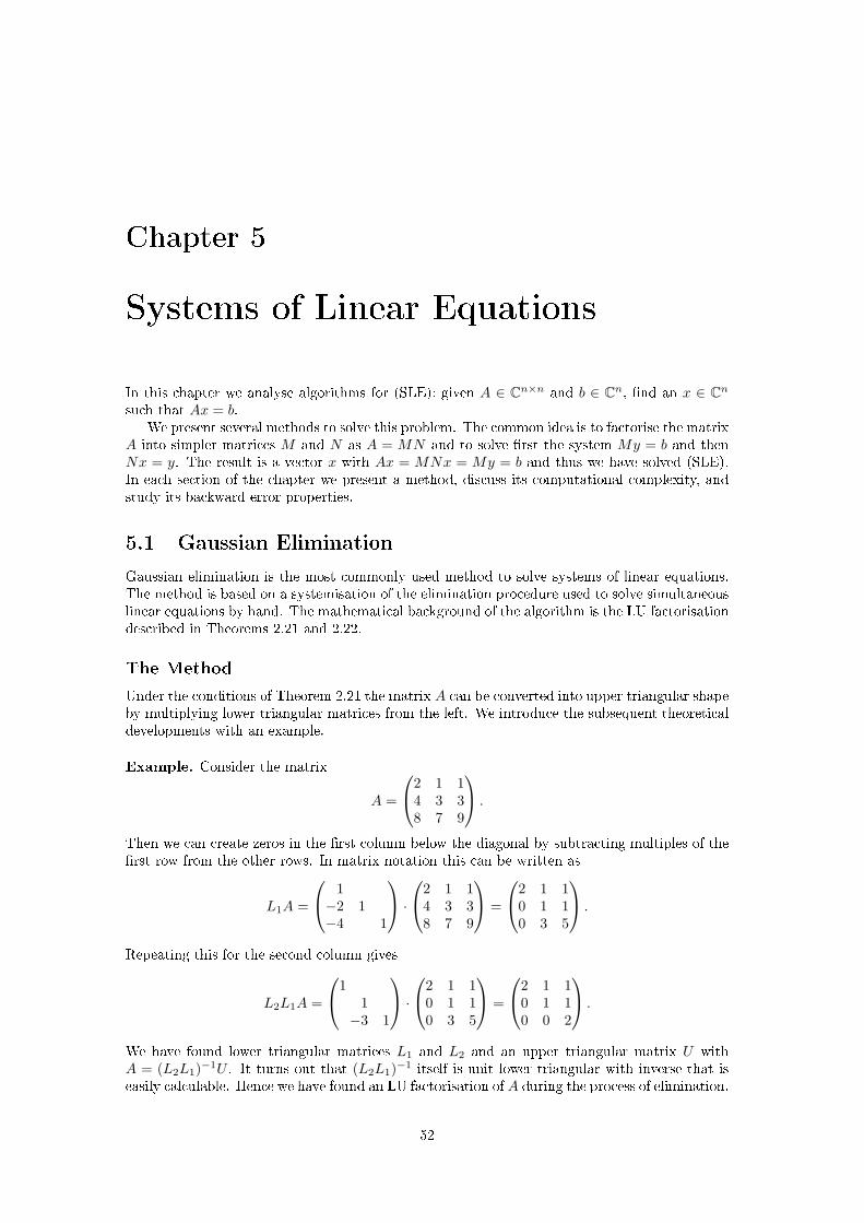
Chapter 5
Systems of Linear Equations
In this chapter we analyse algorithms for (SLE): given A ∈ Cn×n and b ∈ Cn, nd an x ∈ Cnsuch that Ax = b.
We present several methods to solve this problem. The common idea is to factorise the matrixA into simpler matrices M and N as A = MN and to solve rst the system My = b and thenNx = y. The result is a vector x with Ax = MNx = My = b and thus we have solved (SLE).In each section of the chapter we present a method, discuss its computational complexity, andstudy its backward error properties.
5.1 Gaussian Elimination
Gaussian elimination is the most commonly used method to solve systems of linear equations.The method is based on a systemisation of the elimination procedure used to solve simultaneouslinear equations by hand. The mathematical background of the algorithm is the LU factorisationdescribed in Theorems 2.21 and 2.22.
The Method
Under the conditions of Theorem 2.21 the matrix A can be converted into upper triangular shapeby multiplying lower triangular matrices from the left. We introduce the subsequent theoreticaldevelopments with an example.
Example. Consider the matrix
A =
2 1 14 3 38 7 9
.
Then we can create zeros in the rst column below the diagonal by subtracting multiples of therst row from the other rows. In matrix notation this can be written as
L1A =
1−2 1−4 1
·2 1 1
4 3 38 7 9
=
2 1 10 1 10 3 5
.
Repeating this for the second column gives
L2L1A =
11−3 1
·2 1 1
0 1 10 3 5
=
2 1 10 1 10 0 2
.
We have found lower triangular matrices L1 and L2 and an upper triangular matrix U withA = (L2L1)−1U . It turns out that (L2L1)−1 itself is unit lower triangular with inverse that iseasily calculable. Hence we have found an LU factorisation of A during the process of elimination.
52
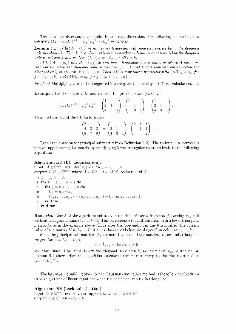
The ideas in this example generalise to arbitrary dimension. The following lemma helps tocalculate (Lk · · ·L2L1)−1 = L−1
1 L−12 · · ·L
−1k in general.
Lemma 5.1. a) Let L = (`ij) be unit lower triangular with non-zero entries below the diagonalonly in column k. Then L−1 is also unit lower triangular with non-zero entries below the diagonalonly in column k and we have (L−1)ik = −`ik for all i > k.
b) Let A = (aij) and B = (bij) be unit lower triangular n × n matrices where A has non-zero entries below the diagonal only in columns 1, . . . , k and B has non-zero entries below thediagonal only in columns k + 1, . . . , n. Then AB is unit lower triangular with (AB)ij = aij forj ∈ 1, . . . , k and (AB)ij = bij for j ∈ k + 1, . . . , n.
Proof. a) Multiplying L with the suggested inverse gives the identity. b) Direct calculation.
Example. For the matrices L1 and L2 from the previous example we get
(L2L1)−1 = L−11 L−1
2 =
12 14 1
·1
13 1
=
12 14 3 1
.
Thus we have found the LU factorisation2 1 14 3 38 7 9
=
12 14 3 1
·2 1 1
1 12
.
Recall the notation for principal submatrix from Denition 2.20. The technique to convert Ainto an upper triangular matrix by multiplying lower triangular matrices leads to the followingalgorithm:
Algorithm LU (LU factorisation).input: A ∈ Cn×n with det(Aj) 6= 0 for j = 1, . . . , noutput: L,U ∈ Cn×n where A = LU is the LU factorisation of A
1: L = I, U = A2: for k = 1, . . . , n− 1 do3: for j = k + 1, . . . , n do4: ljk = ujk/ukk5: (uj,k, . . . , uj,n) = (uj,k, . . . , uj,n)− lj,k(uk,k, . . . , uk,n)6: end for7: end for
Remarks. Line 5 of the algorithm subtracts a multiple of row k from row j, causing ujk = 0without changing columns 1, . . . , k−1. This corresponds to multiplication with a lower triangularmatrix Lk as in the example above. Thus after the loop ending in line 6 is nished, the currentvalue of the matrix U is Lk · · ·L1A and it has zeros below the diagonal in columns 1, . . . , k.
Since the principal sub-matrices Aj are non-singular and the matrices Lj are unit triangular
we get, for A = Lk · · ·L1A,det Ak+1 = detAk+1 6= 0
and thus, since A has zeros below the diagonal in column k, we must have ukk 6= 0 in line 4.Lemma 5.1 shows that the algorithm calculates the correct entry ljk for the matrix L =(Ln · · ·L1)−1.
The last missing building block for the Gaussian elimination method is the following algorithmto solve systems of linear equations when the coecient matrix is triangular.
Algorithm BS (back substitution).input: U ∈ Cn×n non-singular, upper triangular and b ∈ Cnoutput: x ∈ Cn with Ux = b
53
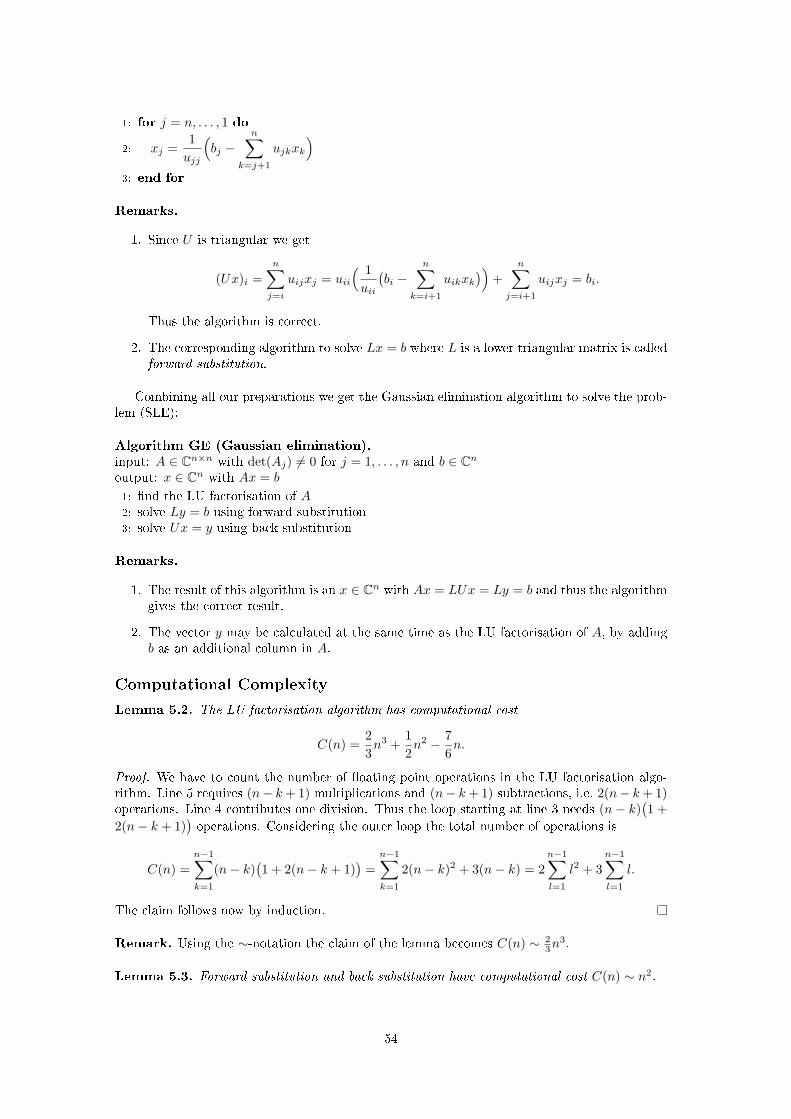
1: for j = n, . . . , 1 do
2: xj =1ujj
(bj −
n∑k=j+1
ujkxk
)3: end for
Remarks.
1. Since U is triangular we get
(Ux)i =n∑j=i
uijxj = uii
( 1uii
(bi −
n∑k=i+1
uikxk))
+n∑
j=i+1
uijxj = bi.
Thus the algorithm is correct.
2. The corresponding algorithm to solve Lx = b where L is a lower triangular matrix is calledforward substitution.
Combining all our preparations we get the Gaussian elimination algorithm to solve the prob-lem (SLE):
Algorithm GE (Gaussian elimination).input: A ∈ Cn×n with det(Aj) 6= 0 for j = 1, . . . , n and b ∈ Cnoutput: x ∈ Cn with Ax = b
1: nd the LU factorisation of A2: solve Ly = b using forward substitution3: solve Ux = y using back substitution
Remarks.
1. The result of this algorithm is an x ∈ Cn with Ax = LUx = Ly = b and thus the algorithmgives the correct result.
2. The vector y may be calculated at the same time as the LU factorisation of A, by addingb as an additional column in A.
Computational Complexity
Lemma 5.2. The LU factorisation algorithm has computational cost
C(n) =23n3 +
12n2 − 7
6n.
Proof. We have to count the number of oating point operations in the LU factorisation algo-rithm. Line 5 requires (n− k+ 1) multiplications and (n− k+ 1) subtractions, i.e. 2(n− k+ 1)operations. Line 4 contributes one division. Thus the loop starting at line 3 needs (n− k)
(1 +
2(n− k + 1))operations. Considering the outer loop the total number of operations is
C(n) =n−1∑k=1
(n− k)(1 + 2(n− k + 1)
)=n−1∑k=1
2(n− k)2 + 3(n− k) = 2n−1∑l=1
l2 + 3n−1∑l=1
l.
The claim follows now by induction.
Remark. Using the ∼-notation the claim of the lemma becomes C(n) ∼ 23n
3.
Lemma 5.3. Forward substitution and back substitution have computational cost C(n) ∼ n2.
54
Proof. Calculating xj in the back substitution algorithm needs 2(n − j) + 1 operations. Thusthe total cost is
C(n) =n∑j=1
(2(n− j) + 1
)= 2
n−1∑k=0
k + n = n(n− 1) + n = n2.
A similar argument applies to the situation of forward substitution.
Theorem 5.4 (Computational Complexity of Gaussian Elimination). The asymptotic compu-tational cost of the GE algorithm is of order
C(n) ∼ 23n3.
Proof. This is an immediate consequence of the previous two lemmas.
Error Analysis
The following theorem is proved by using the Assumptions (A1) and (A2) concerning computerarithmetic. The proof is somewhat involved and we omit it here. We include the statement,however, because it is an important building block in the overall understanding of backwarderror analysis for Gaussian elimination. We use the notation | · | for matrices, introduced justprior to Lemma 1.34.
Theorem 5.5. The forward and back substitution algorithms are backward stable: the computedsolution x of a triangular system of equations Tx = b satises (T+∆T )x = b for some triangularmatrix ∆T ∈ Cn×n with, for εm suciently small,
|∆T | ≤ nεm
1− nεm|T |.
Note that this theorem implies that ∆T has the same triangular structure as T itself. Theresult shows that, for nεm suciently small, there is a constant c independent of n such that,by Lemma 1.34,
‖∆T‖∞ ≤ cnεm‖T‖∞.
Applying this result to backsubstitution we nd that the computed solution of Ux = y, x, solves(U + ∆U)x = y and that
‖∆U‖∞ ≤ cnεm‖U‖∞.
Using Proposition 3.5 about the conditioning of (SLE) we get an upper bound on the error inthe computed result of back substitution:
‖x− x‖∞‖x‖∞
≤ cκ(U)nεm
for κ(U)nεm suciently small.Thus the backward substitution step of Gaussian elimination is numerically stable and does
not introduces large errors, provided κ(U)nεm remains small. The same holds for forwardsubstitution. The LU factorisation algorithm, however, is not backward stable. To explain thisfact we describe two more results from backward error analysis.
Theorem 5.6. The computed LU -factors in a Gaussian elimination of A ∈ Rn×n, L and U ,satisfy
LU = A+ ∆A
where, for εm suciently small,
|∆A| ≤ nεm
1− nεm|L||U |.
55

The proof of this result is similar to that of the previous theorem, and we omit it too.Combining the two previous theorems gives the following backward error analysis result for thesolution of (SLE) by Gaussian elimnation.
Theorem 5.7. Let x be the approximate solution of (SLE) as computed by algorithm GE. Then
(A+ ∆A)x = b
where, for εm suciently small,
|∆A| ≤ 3nεm
1− 3nεm|L||U |.
Proof. See Exercise 5-10.
This would give a backward stability result if it were possible to bound ‖|L||U |‖ in terms of‖A‖. Unfortunately this is not possible as we illustrate in the following example.
Example. [Eect of Rounding] Let
A =(ε 11 1
)for some ε > 0. Then A has a LU factorisation A = LU with
L =(
1 0ε−1 1
), U =
(ε 10 1− ε−1
).
Now assume ε 1. Then ε−1 is a huge number and the representation of these matrices storedin a computer will be rounded. The matrices might be represented as
L =(
1 0ε−1 1
), U =
(ε 10 −ε−1
),
which is compatible with Assumption (A1) on rounding errors. We have L = L and U ≈ U .But multiplying the two rounded matrices gives
LU =(ε 11 0
)= A+
(0 00 −1
)︸ ︷︷ ︸
∆A
.
A small rounding error leads to a large backward error ∆A. The example shows that for Gaussianelimination a backward error analysis will, in general, lead to the conclusion that the perturbedproblem is not close to the original one: the algorithm is not backward stable.
Discussing the result in terms of the previous theorem, note that ‖A‖∞ = 2 and that‖|L||U |‖∞ = Θ(ε−1). Hence it is not possible to bound ‖|L||U |‖ in terms of ‖A‖, indepen-dently of ε.
Note that this problem is not related to the conditioning of the matrix A. We have
A−1 = (1− ε)−1
(−1 11 −ε
)and thus κ(A) = ‖A‖∞‖A−1‖∞ ≈ 4 for small ε > 0 and the matrix A is well conditioned.
5.2 Gaussian Elimination with Partial Pivoting
Because of the instability illustrated in the previous example, the classical Gaussian eliminationmethod is not used in black box numerical software for (SLE). However, the continuation of theexample illustrates the resolution: permutations can cure this problem.
56

Example. [Eect of Rounding Continued] Let
P =(
0 11 0
), and A′ = PA =
(1 1ε 1
),
then
L′ =(
1 0ε 1
)U ′ =
(1 10 1− ε
)L′ =
(1 0ε 1
)U ′ =
(1 10 1
).
Thus
L′U ′ =(
1 1ε 1 + ε
)= A′ +
(0 00 ε
)︸ ︷︷ ︸
∆A′
,
and the backward error ∆A′ is small.
Thus permuting is important. There are two primary methods of permutation:
GEPP Swap rows only to maximise |a(l)ll | over all choices from l, . . . , n: (n− l + 1) of them.
GECP Swap rows and columns to maximise |a(l)ll | over all choices from l, . . . , n: (n− l+ 1)2 of
them.
Here GEPP denotes Gaussian Elimination with partial pivoting whilst GECP denotes Gaus-sian Elimination with complete pivoting. GEPP is the most widely used in practice and so wedevote most of our analysis to this algorithm.
The Method
The instability of Gaussian elimination highlighted above is caused by the fact that we divide bythe tiny number ukk = ε in step 4 of the LU factorisation algorithm. Motivated by the resolutionin the example above, we will avoid this problem in the improved version of the algorithm byrearranging rows k, . . . , n by multiplication with a permutation matrix at the beginning of thekth iteration in order to maximise the element ukk. The following argument shows that themodied algorithm still works correctly.
We want to calculateU = Ln−1Pn−1 · · ·L1P1A.
Multiplying the permutation matrix Pk from the left exchanges rows k and ik where ik is chosenfrom k, . . . , n to maximise the element uikk. We can rewrite this as
U = L′n−1 · · ·L′1 Pn−1 · · ·P1A
where L′n−1 = Ln−1 and
L′k = Pn−1 · · ·Pk+1LkP−1k+1 · · ·P
−1n−1
for k = 1, . . . , n−2. Since Pn−1 · · ·Pk+1 exchanges rows k+1, . . . , n and P−1k+1 · · ·P
−1n−1 performs
the corresponding permutation on the columns k + 1, . . . , n the shape of L′k is the same as theshape of Lk: it is unit lower triangular and the only non-vanishing entries below the diagonalare in column k. Hence we can still use Lemma 5.1 to calculate L = (L′n−1 · · ·L′1)−1. The abovearguments lead to the following algorithm.
Algorithm LUPP (LU factorisation with partial pivoting).input: A ∈ Cn×n non-singularoutput: L,U, P ∈ Cn×n where PA = LU with L unit lower triangular,
U non-singular upper triangular and P a permutation matrix
57

1: U = A, L = I, P = I2: for k = 1, . . . , n− 1 do3: choose i ∈ k, . . . , n which maximises |uik|4: exchange row (uk,k, . . . , uk,n) with (ui,k, . . . , ui,n)5: exchange row (lk,1, . . . , lk,k−1) with (li,1, . . . , li,k−1)6: exchange row (pk,1, . . . , pk,n) with (pi,1, . . . , pi,n)7: for j = k + 1, . . . , n do8: ljk = ujk/ukk9: (uj,k, . . . , uj,n) = (uj,k, . . . , uj,n)− lj,k(uk,k, . . . , uk,n)
10: end for11: end for
Remark. One can show that, whenever A is non-singular, the element ukk is always non-zeroafter the row-exchange. Thus we do no longer require the condition det(Aj) 6= 0 to avoid adivision by zero here.
Lemma 5.8. The resulting matrices L and Lk satisfy ‖L‖∞ ≤ n and ‖Lk‖∞ ≤ 2.
Proof. Each matrix Lk has entries |(Lk)ij | ≤ 1 for all i, j ∈ 1, . . . , n. Consequently the sameis true of L. The result for ‖L‖∞ follows directly. Furthermore, as each row of Lk contains atmost two non-zero entries, we have ‖Lk‖∞ ≤ 2.
Gaussian elimination with partial pivoting now works as follows:
Algorithm GEPP (Gaussian elimination with partial pivoting).input: A ∈ Cn×n non-singular, b ∈ Cnoutput: x ∈ Cn with Ax = b
1: nd PA = LU using algorithm LUPP2: solve Ly = Pb using forward substitution3: solve Ux = y using back substitution
Remarks.
1. The result of this algorithm is an x ∈ Cn with Ax = P−1LUx = P−1Ly = P−1Pb = band thus the algorithm is correct.
2. Again it is possible to compute y by appending b as an extra column in the matrix A.
Computational Complexity
The computational complexity is the same as for the LU algorithm given in Theorem 5.4. Thisfollows from the fact that we only added steps to exchange rows in the LU algorithm and suchexchanges do not incur computational cost in our model. If we assign unit cost to the comparisonsbetween number, made to maximise |uik| in step 3 of the algorithm, then this added additionalcost is of order Θ(n2); thus it can be neglected for a Θ(n3) algorithm. For GECP the additionalcost is of order Θ(n3) and hence cannot be neglected.
Error Analysis
To derive a backward error analysis for GEPP is nontrivial. We limit ourselves to an heuristicunderstanding of the analysis, based on the following two assumptions:
• The computed permutation matrix P is the correct permutation P ;
• The computed L,U factors L, U are well approximated by L,U .
58

Then applying Theorem 5.7 to PA = PA we obtain a computed solution x which satises
P (A+ ∆A)x = Pb
where
‖∆A‖∞ ≤3nεm
1− 3nεm‖L‖∞‖U‖∞.
To bound the right-hand side of this expression we use the following denition:
Denition 5.9. Dene gn(A), the growth factor for matrix A ∈ Cn×n, by
gn(A) =‖U‖max
‖A‖max. (5.1)
From this it follows, by Lemma 1.35, that
‖U‖∞ ≤ ngn(A)‖A‖∞.
We also have ‖L‖∞ ≤ n and hence, using the approximation L ≈ L, U ≈ U ,
‖∆A‖∞ .3n3gn(A)εm
1− 3nεm‖A‖∞. (5.2)
(Here . indicates that approximations have been made in deriving the inequality). To under-stand the implications of this bound we study the behaviour of the growth factor in furtherdetail.
Lemma 5.10. The growth factor gn(A) satises gn(A) ≤ 2n−1 for every A ∈ Cn×n.
Proof. We have U = L′n−1 · · ·L′1PA. For any k ∈ 1, . . . , n − 1 and any matrix A ∈ Cn×n wend
‖L′kA‖max = maxi,j
∣∣(L′kA)ij∣∣
= maxi,j=1,...,n
∣∣ n∑l=1
(L′k)ilalj∣∣
≤ maxi=1,...,n
∣∣ n∑l=1
(L′k)il∣∣ max
i,j|aij |
= ‖L′k‖∞‖A‖max
≤ 2‖A‖max
and thus by applying the matrices L′1, . . . L′n−1 in order we get, since ‖PA‖max = ‖A‖max,
‖U‖max ≤ 2n−1 maxi,j ‖A‖max. This completes the proof.
Placing this upper-bound on gn(A) in (5.2) shows a worryingly large n-dependence in thebackward error bound for GEPP:
‖∆A‖∞ .3n32n−1εm
1− 3nεm‖A‖∞.
Furthermore, the following example shows that the upper bound on gn(A) from the lemma canbe attained.
Example. Let
A =
1 1−1 1 1−1 −1 1 1...
.... . .
. . ....
−1 −1 · · · −1 1
∈ Rn×n.
59
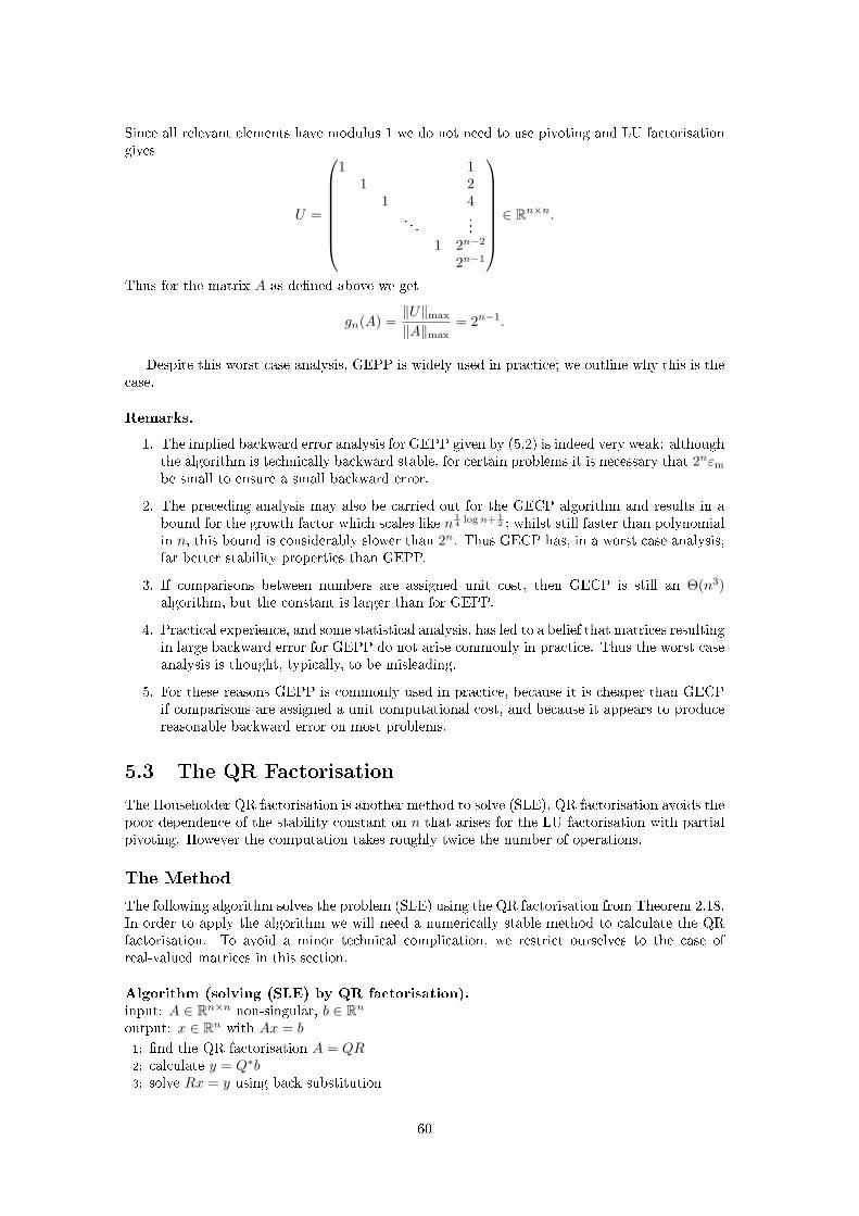
Since all relevant elements have modulus 1 we do not need to use pivoting and LU factorisationgives
U =
1 11 2
1 4. . .
...1 2n−2
2n−1
∈ Rn×n.
Thus for the matrix A as dened above we get
gn(A) =‖U‖max
‖A‖max= 2n−1.
Despite this worst case analysis, GEPP is widely used in practice; we outline why this is thecase.
Remarks.
1. The implied backward error analysis for GEPP given by (5.2) is indeed very weak: althoughthe algorithm is technically backward stable, for certain problems it is necessary that 2nεm
be small to ensure a small backward error.
2. The preceding analysis may also be carried out for the GECP algorithm and results in abound for the growth factor which scales like n
14 logn+ 1
2 ; whilst still faster than polynomialin n, this bound is considerably slower than 2n. Thus GECP has, in a worst case analysis,far better stability properties than GEPP.
3. If comparisons between numbers are assigned unit cost, then GECP is still an Θ(n3)algorithm, but the constant is larger than for GEPP.
4. Practical experience, and some statistical analysis, has led to a belief that matrices resultingin large backward error for GEPP do not arise commonly in practice. Thus the worst caseanalysis is thought, typically, to be misleading.
5. For these reasons GEPP is commonly used in practice, because it is cheaper than GECPif comparisons are assigned a unit computational cost, and because it appears to producereasonable backward error on most problems.
5.3 The QR Factorisation
The Householder QR factorisation is another method to solve (SLE). QR factorisation avoids thepoor dependence of the stability constant on n that arises for the LU factorisation with partialpivoting. However the computation takes roughly twice the number of operations.
The Method
The following algorithm solves the problem (SLE) using the QR factorisation from Theorem 2.18.In order to apply the algorithm we will need a numerically stable method to calculate the QRfactorisation. To avoid a minor technical complication, we restrict ourselves to the case ofreal-valued matrices in this section.
Algorithm (solving (SLE) by QR factorisation).input: A ∈ Rn×n non-singular, b ∈ Rnoutput: x ∈ Rn with Ax = b
1: nd the QR factorisation A = QR2: calculate y = Q∗b3: solve Rx = y using back substitution
60

The result of this algorithm is an x ∈ Rn with Ax = QRx = Qy = QQ∗b = b and thus thealgorithm is correct. To calculate the QR factorisation we will use the following algorithm. Wepresent the full algorithm rst and then analyse it to see how it works. The algorithm uses thesign function, which is dened as follows.
sign(x) =
+1, if x ≥ 0, and−1 else.
Algorithm QR (Householder QR factorisation).input: A ∈ Rm×n with m ≥ noutput: Q ∈ Rm×m orthogonal, R ∈ Rm×n upper triangular with A = QR
1: Q = I, R = A2: for k = 1, . . . , n do3: u = (rkk, . . . , rmk) ∈ Rm−k+1
4: v = sign(u1)‖u‖2e1 + u where e1 = (1, 0, . . . , 0) ∈ Rm−k+1
5: v = v/‖v‖26: Hk = (Im−k+1 − 2vv∗) ∈ R(m−k+1)×(m−k+1)
7: Qk =(Ik−1 0
0 Hk
)8: R = Qk ·R9: Q = Q ·Qk
10: end for
Remarks.
1. This method of calculating a QR factorisation has very desirable numerical stability prop-erties.
2. The algorithm calculates matrices Qk with Qk = Q∗k for k = 1, . . . , n − 1 as well asR = Qn−1 · · ·Q1A and Q = Q1 · · ·Qn−1.
3. We will see that Qk · · ·Q1A has zeros below the diagonal in columns 1, . . . , k and thus thenal result R = Qn−1 · · ·Q1A is upper triangular.
4. The only use we make of the matrix Q when solving (SLE) by QR factorisation is tocalculate Q∗b. Thus for solving (SLE) we can omit the explicit calculation of Q by replacingline 9 of algorithm QR with the statement b = Qkb. The nal result in the variable b willthen be
Qn−1 · · ·Q1b = (Q1 · · ·Qn−1)∗b = Q∗b.
Householder Reections
In step 8 of algorithm QR we calculate a product of the form
Qk ·(R11 R12
0 R22
)=(R11 R12
0 HkR22
)(5.3)
where R11 ∈ R(k−1)×(k−1) and Hk, R22 ∈ R(m−k+1)×(m−k+1). The purpose of this subsection isto understand this step of the algorithm.
If Hk as calculated in step 6 of algorithm QR is applied to a vector x ∈ Rm−k+1 the result is
Hkx = x− 2vv∗x = x− 2v〈v, x〉.
Since the vector v〈v, x〉 is the projection of x onto v, the value x − v〈v, x〉 is the projection ofx onto the plane which is orthogonal to v and x − 2v〈v, x〉 is the reection of x at that plane.Reecting twice at the same plane gives back the original vector and thus we nd
H∗kHk = HkHk = I.
61
This shows that the matrices Hk, and then also Qk, are orthogonal for every k ∈ 1, . . . , n− 1.The vector which denes the reection plane is either v = u− ‖u‖2e1 or v = u− (−‖u‖2e1),
depending on the sign of u1. The corresponding reection maps the vector u to Hku = ‖u‖2e1
or Hku = −‖u‖2e1 respectively. In either case the image is a multiple of e1 and since u is therst column of the matrix block R22 the product HkR22 has zeros below the diagonal in therst column. The rst column of R22 is the kth column of R and thus QkR has zeros belowthe diagonal in columns 1, . . . , k. For k = n − 1 we nd that R = Qn−1 · · ·Q1A is an uppertriangular matrix as required.
Remarks.
1. The matrices Hk and sometimes also Qk are called Householder reections.
2. The choice of sign in the denition of u helps to increase the stability of the algorithm inthe cases u ≈ ‖u‖2e1 and u ≈ −‖u‖2e1. In the complex case, sign(x) will be replaced bya complex number σ ∈ C with |σ| = 1.
Computational Complexity
We considered two variants of algorithm QR, either calculating the full matrix Q as formulatedin line 9 of the algorithm or only calculating Q∗b by replacing line 9 with the statement b = Qkb.We handle the dierent cases by rst analysing the operation count for the algorithm with line 9omitted.
Lemma 5.11. The computational cost C(m,n) for algorithm QR applied to an m × n-matrixwithout calculating Q or Q∗b is asymptotically
C(m,n) ∼ 2mn2 − 23n3 for m,n→∞ with m = Θ(n).
Proof. We count the number of operations for the individual steps of algorithm QR. Fromequation (5.3) we can see that for calculating the product QkR in step 8 we only have tocalculate HkR22 = R22 − 2vv∗R22. Since v = v/‖v‖2 and ‖v‖2 =
√v∗v we can calculate this as
HkR22 = R22 −v
v∗v/2v∗R22.
Using this formula we get the following operations count:
• construction of v: 2(m− k + 1) + 1 operations (counting√· as 1).
• computing v∗R22: Since each of the n − k + 1 components of the matrix-vector prod-uct v∗R22 needs m− k+ 1 multiplications and m− k additions, the computation of v∗R22
requires (n− k + 1)((m− k + 1) + (m− k)
)operations.
• Calculating v∗v/2 needs 2(m − k + 1) operations and dividing v by the result requiresanother (m− k + 1) divisions.
• Calculating (· · · )(v∗R22) from this needs (m− k + 1)(n− k + 1) multiplications.
• Calculating R22 − (· · · ) requires (m− k + 1)(n− k + 1) subtractions.
Thus the total operation count is
C(m,n) =n∑k=1
5(m− k + 1) + 1 + (n− k + 1)(4(m− k + 1)− 1
)=
m∑l=m−n+1
5l + 1 + (n−m+ l)(4l − 1)
= 2mn2 − 23n3 + terms with at most two factors m,n
∼ 2mn2 − 23n3
62

for m,n→∞ with m = Θ(n).
If we need to calculate the full matrix Q we have to perform an (m − k + 1) × (m − k + 1)matrix-matrix multiplication in step 9. Assuming that we use the standard matrix multiplicationalgorithm this contributes asymptotic cost Θ(m3) and so the asymptotic cost of algorithm QRwill be increased by this step. But if we apply algorithm QR only to solve (SLE), we just haveto calculate Q∗b instead of Q. Algorithmically this is the same as appending the vector b as anadditional column to the matrix A. Thus the computational cost for this algorithm is C(m,n+1)and since
2m(n+ 1)2 − 23
(n+ 1)3 ∼ 2mn2 − 23n3
for m,n → ∞ with m = Θ(n) the asymptotic cost does not change. For solving (SLE) we alsohave m = n and thus we nd that the asymptotic computational cost of solving (SLE) usingHouseholder QR factorisation is
C(n) ∼ 2nn2 − 23n3 =
43n3 for n→∞.
This analysis shows that solving (SLE) using Householder QR factorisation requires asymp-totically double the number of steps than algorithm GEPP does. This is the price we have topay for the better stability properties of the QR algorithm.
Error Analysis
The backward error analysis for Householder QR is best expressed in terms of the norms ofmatrix columns. For any matrix D ∈ Rn×n we write dj to denote the jth column of D. Asimilar convention for upper and lower case letters is used in what follows.
The rst result concerns the form of the triangular factor in the HouseholderQR factorisation.
Theorem 5.12. Let R denote the computed upper triangular factor in a Householder QR fac-torisation of A ∈ Rn×n. Then there exists orthogonal Q ∈ Rn×n and constant c ∈ R+ suchthat
A+ ∆A = QR
where, for εm suciently small,
‖∆aj‖2 ≤cn2εm
1− cn2εm‖aj‖2, j = 1, . . . , n.
This result can be used to show the following.
Theorem 5.13. Let x solve Ax = b and let x be the solution computed through HouseholderQR. Then
(A+ ∆A)x = b+ ∆b,
where, for some constant c ∈ R+ and for εm suciently small,
‖∆aj‖2 ≤cn2εm
1− cn2εm‖aj‖2,
‖∆b‖2 ≤cn2εm
1− cn2εm‖b‖2.
This is a considerable improvement over the worst case analysis for GEPP. However, as wehave seen, the worst case analysis does not give a true picture of the stability of GEPP inpractice; furthermore, Householder QR costs twice as much as GEPP. Consequently GEPP isfavoured in practice.
63
Bibliography
The book [Hig02] is an excellent source of material concerning backward error analysis for nu-merical algorithms. In particular, proofs of Theorems 5.5, 5.6, 5.12 and 5.13 may all be foundin this book. The fact that the worst case analysis of GEPP does not seem to arise often inpractice is discussed in [TB97].
Exercises
Exercise 5-1. The purpose of this question is to illustrate some of the content of the chapterby means of some Matlab experiments. We consider the linear system
Ax = b (5.4)
where A ∈ Rn×n, b ∈ Rn are given and x ∈ Rn is to be found. In Matlab we start by creatinga random matrix A and vector b. Type
>> A=randn(5)
>> b=randn(5,1)
These two commands will produce a random 5 × 5 matrix and 5-vector where each entry isindependent of all others and is distributed normally with mean 0 and variance 1. Now type
>> x=A\b
This x is the (computer approximation) to the solution of (5.4). To verify this type
>> r=A*x-b; rn=norm(r)
which will produce the norm of the residual r between Ax (with the computed x) and b. Howbig is rn? What does this tell you?
Now we try and explain how Matlab solved (5.4). Type
>> [L,U,P]=lu(A)
and describe what special properties L,U and P have. In particular, what eect does P havewhen applied to an arbitrary 5× 5 matrix? Why is P−1 = PT ? If you type
>> P*A
and then
>> L*U
you see that PA = LU (approximately use norm to measure the residual). Thus, applying Pto (5.4), we see that x solves
LUx = Pb.
Thusx = U−1L−1Pb.
What special features do U and L have which make this a good way to nd x? (Think aboutwhat is involved in solving an arbitrary linear system and compare it to what is involved if thematrix to be inverted has the form of U or L).
The LU factorisation described above is what Matlab uses to solve (5.4) (unless A is sym-metric with positive diagonal entries, in which case Cholesky factorisation is used). But analternative is to use the QR factorisation which we now outline. Type
>> [Q,R]=qr(A)
and then type
64
>> rn=norm(Q*R-A)
noting that this shows that QR is a (approximate) factorisation of A. R has a property youhave seen on another matrix in this question (what is it?) and is hence easy to invert. Whatabout Q? Let us extract the columns from Q. Type
>> q1=Q(1:5,1); q2=Q(1:5,2); q3=Q(1:5,3); q4=Q(1:5,4); q5=Q(1:5,5)
What do these vectors q represent? Now, using the Matlab command dot(a,b), which calculatesdot products of vectors, experiment with the properties of inner-products amongst the q vectors.What do you nd? Why is Q easy to invert?
Using this QR factorisation it is possible to nd x solving (5.4) as x = R−1Q−1b. Althoughthis method is not often used it has some nice mathematical properties which we will explain inthe lectures.
Exercise 5-2. In analogy to the back substitution algorithm formulate the forward substitutionalgorithm to solve Ly = b where L ∈ Cn×n is a lower triangular, invertible matrix and b ∈ Cnis a vector. Show that your algorithm computes the correct result and that it has asymptoticcomputational cost of order Θ(n2).
Exercise 5-3. a) Find the LU factorisation of
A =(
1 23 1
).
What is the growth factor gn(A) in this case? b) Find a QR factorisation of the same matrix,using both Gram-Schmidt and Householder. c) Find the condition number of A in the ‖ · ‖∞,‖ · ‖2 and ‖ · ‖1 norms.
Exercise 5-4. a) Let A = a⊗b. Find all eigenvalues and eigenvectors of A. When is A a normalmatrix? b) Let H ∈ Rn×n be a Householder reection. Show that H has a single eigenvalue at−1 and an eigenvalue +1 of multiplicity (n− 1). What is the value of det(H)?
Exercise 5-5. Determine the asymptotic computational cost of algorithm QR when calculatingthe full matrix Q.
Exercise 5-6. Write a Matlab algorithms to solve
Ux = y
Ly = b
where U ∈ Rn×n (resp. L ∈ Rn×n) is an upper (resp. lower) triangular matrix. Constructexamples U and y where you know the exact solution x (for some large n). Compute x usingyour algorithm and study the error
e =‖x− x‖‖x‖
,
discussing your results.Now generate a random upper triangular U ∈ R50×50 with non-zero entries uniformly dis-
tributed in [−1, 1]. Let x = (1, . . . , 1)T ∈ R50 and compute y = Ux by use of Matlab's matrixmultiply. Solve Ux = y (with the just computed y) using the algorithm you designed above andcompute the relative error
e =‖x− x‖∞‖x‖∞
.
Do this several hundred times and discuss the resulting statistics of e.
Exercise 5-7. Using the construction from Exercise 2-2 as the basis for an algorithm, andmaking maximum use of symmetry, show that Cholesky factorisation of a symmetric positive-denite matrix can be achieved in approximately half the ops of standard Gaussian Elimination.
65
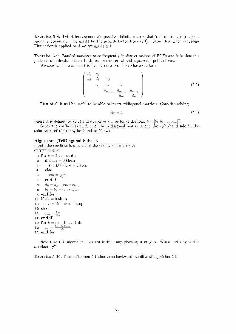
Exercise 5-8. Let A be a symmetric positive denite matrix that is also strongly (row) di-agonally dominant. Let gn(A) be the growth factor from (5.1). Show that when GaussianElmination is applied to A we get gn(A) ≤ 1.
Exercise 5-9. Banded matrices arise frequently in discretisations of PDEs and it is thus im-portant to understand them both from a theoretical and a practical point of view.
We consider here m×m tridiagonal matrices. These have the formd1 c1a2 d2 c2
. . .. . .
. . .
am−1 dm−1 cm−1
am dm
(5.5)
First of all it will be useful to be able to invert tridiagonal matrices. Consider solving
Ax = b, (5.6)
where A is dened by (5.5) and b is an m× 1 vector of the form b = [b1, b2, . . . , bm]T .Given the coecients ai, di, ci of the tridiagonal matrix A and the right-hand side bi, the
solution xi of (5.6) may be found as follows.
Algorithm (TriDiagonal Solver).input: the coecients ai, di, ci of the tridiagonal matrix Aoutput: x ∈ Rn
1: for k = 2, . . . ,m do2: if dk−1 = 0 then3: signal failure and stop4: else5: rm = ak
dk−1
6: end if7: dk = dk − rm ∗ ck−1
8: bk = bk − rm ∗ bk−1
9: end for10: if dn = 0 then11: signal failure and stop12: else13: xm = bm
dm
14: end if15: for k = m− 1, . . . , 1 do16: xk = bk−ckxk+1
dk
17: end for
Note that this algorithm does not include any pivoting strategies. When and why is thissatisfactory?
Exercise 5-10. Prove Theorem 5.7 about the backward stability of algorithm GE.
66
Chapter 6
Iterative Methods
In the previous chapter we considered methods which directly solve (SLE) using Θ(n3) opera-tions. In this chapter we will introduce iterative methods. These methods construct a sequence(xk)k∈N with
xk → x for k →∞,
where x solves (SLE). These methods approximate the exact solution x by the computed valuexk for large k and thus, even in the absence of rounding errors, the resulting algorithms onlycompute approximate solutions to (SLE). In practical applications this is no problem, since onecan choose k large enough such that the approximation error is of the same order of magnitudeas the deviation caused by rounding errors in the exact methods.
The primary motivation for the use of such iterative methods arises for problems whereA ∈ Cn×n with n 1, so that solving the problem by the direct methods of Chapter 5, withcost Θ(n3), is prohibitively expensive. If A has some special structure, for example if matrix-vector multiplication with A is cheap to calculate, then iterative methods can have a substantialadvantage over direct methods.
For the methods considered in this chapter, the sequence (xk) is constructed iteratively, i.e.starting with a value x0 the value xk, for each k, is computed from xk−1. The map xk−1 7→ xkmay be either linear or nonlinear; we discuss methods of both types. The two competing criteriafor the iteration are:
• The calculation of xk from xk−1 should be cheap, relative to the cost of solving (SLE).
• The convergence of xk to x should be fast.
These two criteria are often contradictory to one another and the trade-o between them is verymuch dependent upon the matrix A itself. To illustrate this trade o it is useful to have thefollowing two extreme iterative methods in mind:
• xk = A−1b; and
• xk = xk−1.
The rst is not cheap to implement each step involves solving (SLE) by a direct method,and our assumption is that this is prohibitively expensive but converges fast: in one step.The second is cheap to implement but does not converge at all. Successful iterative methods liesomewhere between these extremes.
In many cases, the cost of computing xk from xk−1 is dominated by the cost of matrix-vectormultiplication for a matrix N which is derived from A. The resulting methods will be ecient ifthese multiplications can be computed eciently. The most common structure leading to cheapmatrix-vector multiplication is sparsity : where A has only a small number of non-zero entries.Then matrix-vector multiplication by A, A∗ or any matrix N where N inherits the sparsity ofA will be cheap; the matrix N might, for example, be formed from the o-diagonals of A.
In this chapter we will focus only on errors incurred through using a nite number of iterationsbut we will not discuss the eect of rounding errors. For each section describing a computational
67
approach there will be three subsections, one dening the method, the second studying error asa function of the number of iterations k, and the third discussing computational cost. We willconsider the cost of achieving an error of size ε. We will show that, for some important problems,it is possible to compute an approximate solution in time Θ(na) with a < 3 as the dimension nof the problem increases, thus beating the cost of the direct methods from the previous chapter.
6.1 Linear Methods
Iterative methods where xk is computed from xk−1 by application of a linear map are calledlinear methods. In this section we describe results about linear methods in general. Sections 6.2and 6.3 below introduce two specic instances of linear methods, namely the Jacobi method andthe successive over relaxation scheme (SOR).
The Method
The basic idea of the methods described in this section is to write the matrix A as A = M +Nwhere the matrix M is easier to invert than A. Then, given xk−1, we can dene xk by
Mxk = b−Nxk−1. (6.1)
If we assume for the moment that limk→∞ xk = x, then the limit x satises
Mx = limk→∞
Mxk = limk→∞
(b−Nxk−1) = b−Nx
and thus we get Ax = b. This shows that the only possible limit for this sequence is the solutionof (SLE). Thus, once we know that the generated sequence converges for a given matrix Aand a given initial value x0, we can iteratively compute xk for a big value of k to get anapproximation for x. In the following sections we will give sucient criteria for convergence ofthe sequence (xk)k∈N.
This leads to the following algorithm.
Algorithm LI (linear iterative methods).input: A = M +N ∈ Cn×n, b ∈ Cn, x0 ∈ Cnoutput: xk ∈ Cn with Axk ≈ b1: for k = 1, 2, 3, . . . do2: compute yk = b−Nxk−1
3: solve Mxk = yk4: end for
To actually implement this method one needs to choose M and N such that the methodconverges (we discuss dierent choices below). One also needs a stopping criterion to decidewhen to quit iterating and to return the resulting approximation xk.
Thus, the remaining problem is to choose a stopping criterion for the iteration. We considerthe error
ek = x− xk,
and the residual vectorrk = b−Axk = Aek
where x is the exact solution of (SLE) and xk the approximation at step k. We would like tochoose k big enough such that ‖ek‖ ≤ ε for a given ε > 0 but, since ek cannot be computedwithout knowledge of the exact solution x, this is not a practical stopping criterion. Instead,we will stop the iteration once ‖rk‖ ≤ εr for some εr > 0. The residual error rk can easily becomputed during the iteration and from the estimate ‖ek‖ = ‖A−1rk‖ ≤ ‖A−1‖‖rk‖ ≤ ‖A−1‖εr
we can get estimates for the error if needed.
68

Error Analysis
Since Mx = b−Nx we get the relation
ek = −M−1Nek−1.
The method converges if ek → 0 for k → ∞. The following lemma characterises convergencewith the help of the spectral radius of the matrix R = −M−1N .
Lemma 6.1. Let R ∈ Cn×n, e0 ∈ Cn and ek = Rke0 for all k ∈ N. Then ek → 0 for all e0 ∈ Cnif and only if ρ(R) < 1.
Proof. Assume rst ρ(R) < 1. Then by Lemma 2.10 we nd an induced matrix norm ‖ · ‖S with‖R‖S < 1 and we get
‖ek‖S = ‖Rke0‖S ≤ ‖R‖kS‖e0‖S −→ 0
for k →∞.On the other hand, if ρ(R) ≥ 1, then there is an e0 ∈ Cn \ 0 with Re0 = λe0 for some
λ ∈ C with |λ| ≥ 1. For this vector e0 we get, in any norm ‖ · ‖,
‖ek‖ = ‖Rke0‖ = |λ|k‖e0‖
and thus ek does not converge to 0 as k →∞.
Remarks.
1. The lemma shows that the linear iterative method dened by (6.1) converges for everyinitial condition x0 ∈ Cn if and only if ρ(R) < 1 for R = −M−1N . The convergence isfast if ρ(R) is small.
2. Since ‖ · ‖ ≥ ρ(·) for every matrix norm ‖ · ‖, a sucient criterion for convergence of aniterative method is ‖R‖ < 1 for any matrix norm ‖ · ‖. On the other hand, whenever themethod converges for every initial condition, there is an induced matrix norm ‖ · ‖ with‖R‖ < 1 by Lemma 2.10.
Computational Complexity
When measuring computational cost for iterative methods it is of interest to know how manyiterations are required to reduce the error to size ε. As before we will consider the relative error‖xk − x‖/‖x‖ = ‖ek‖/‖x‖. By Proposition 3.3 we have
‖ek‖‖x‖
≤ κ(A)‖rk‖‖b‖
. (6.2)
Finding k to achieve‖rk‖‖b‖
≤ ε, (6.3)
and thus‖ek‖‖x‖
≤ κ(A)ε, (6.4)
will lead to an estimate of the computational cost of using the iterative method.Using the relation rk = Aek = ARke0 we can estimate the left hand side of (6.3) to get,
from (6.2),‖ek‖‖x‖
≤ κ(A)‖A‖‖R‖k‖e0‖
‖b‖for any vector norm ‖ · ‖. If ‖ · ‖ is chosen so that ‖R‖ < 1 then choosing k to be the smallestinteger greater than
k] =ln ε−1 + ln ‖A‖+ ln ‖e0‖ − ln ‖b‖
ln ‖R‖−1(6.5)
69
will ensure (6.3).In order to study the dependence of the cost on the dimension n of the problem we consider
a family of matrices A = M +N ∈ Cn×n and vectors b ∈ Cn and also a family of vector normson the spaces Cn. The number k] depends on both ε and n; the n dependence can enter through‖R‖−1, ‖A‖, ‖b‖ and ‖e0‖, but the largest contribution is often through ‖R‖−1, for families ofproblems in which ‖R‖ = 1−Θ(n−β). We incorporate this into the following assumptions, whichlead to a quantication of computational cost.
Assumption 6.2. 1. Calculation of Nx and M−1x together costs Θ(nα) for some α > 0,uniformly for all x ∈ Cn.
2. ‖R‖ = 1−Θ(n−β) for some β > 0.
3. κ(A), ‖A‖, ‖b‖ and ‖e0‖ are bounded uniformly in n.
Theorem 6.3. Under Assumption 6.2 the computational cost to achieve (6.4) by using the lineariterative method is bounded above by cnα+β ln ε−1, for some constant c independent of n and ε.
Proof. The rst item of the assumption ensures that each step of the iteration costs Θ(nα). Thesecond item of the assumption implies that
(ln ‖R‖−1
)−1 = Θ(nβ). Hence combining the secondand third items and using (6.5) gives the desired result.
Remarks.
1. For the theorem to be practically useful, the norm in (6.3) must be readily computable.In some cases ‖R‖ < 1 in some computable norm such as ‖ · ‖∞, ‖ · ‖2 or ‖ · ‖1. Then thepreceding theorem applies directly.
In other cases we only know that ‖R‖S < 1; as the construction of ‖·‖S requires knowledgeof the Jordan Canonical form, this is not a readily computable norm. However, by normequivalence, we know that there is a constant c2 ∈ (0,∞) such that
‖a‖‖b‖≤ c2
‖a‖S‖b‖S
.
The constant c2 may depend on n, but in many important applications this occurs only ina polynomial fashion.
Iterating until we nd a k so that‖rk‖S‖b‖S
≤ ε
c2(6.6)
will ensure‖rk‖‖b‖
≤ ε
and hence (6.4). Finding k to achieve (6.6) will incur cost
knα+β(
ln ε−1 + ln c2(n))
by the methods given in the preceding theorem, if Assumption 6.2 holds in the norm ‖ ·‖S .Thus there is an increase in cost by only a logarithmic factor in n when c2(n) is polynomialin n.
2. In many applications κ(A), ‖A‖ and ‖b‖ do depend upon n, but only polynomially. Againthis leads to an increase in computational cost over the above, but only by a factor whichis logarithmic in n.
70
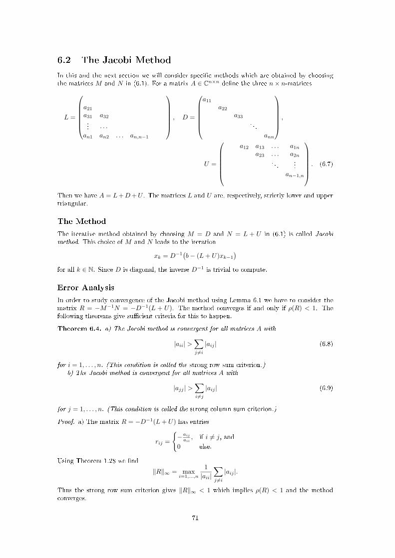
6.2 The Jacobi Method
In this and the next section we will consider specic methods which are obtained by choosingthe matrices M and N in (6.1). For a matrix A ∈ Cn×n dene the three n× n-matrices
L =
a21
a31 a32
... · · ·an1 an2 . . . an,n−1
, D =
a11
a22
a33
. . .
ann
,
U =
a12 a13 . . . a1n
a23 . . . a2n
. . ....
an−1,n
. (6.7)
Then we have A = L+D+U . The matrices L and U are, respectively, strictly lower and uppertriangular.
The Method
The iterative method obtained by choosing M = D and N = L + U in (6.1) is called Jacobimethod. This choice of M and N leads to the iteration
xk = D−1(b− (L+ U)xk−1
)for all k ∈ N. Since D is diagonal, the inverse D−1 is trivial to compute.
Error Analysis
In order to study convergence of the Jacobi method using Lemma 6.1 we have to consider thematrix R = −M−1N = −D−1(L + U). The method converges if and only if ρ(R) < 1. Thefollowing theorems give sucient criteria for this to happen.
Theorem 6.4. a) The Jacobi method is convergent for all matrices A with
|aii| >∑j 6=i
|aij | (6.8)
for i = 1, . . . , n. (This condition is called the strong row sum criterion.)b) The Jacobi method is convergent for all matrices A with
|ajj | >∑i6=j
|aij | (6.9)
for j = 1, . . . , n. (This condition is called the strong column sum criterion.)
Proof. a) The matrix R = −D−1(L+ U) has entries
rij =
−aij
aii, if i 6= j, and
0 else.
Using Theorem 1.28 we nd
‖R‖∞ = maxi=1,...,n
1|aii|
∑j 6=i
|aij |.
Thus the strong row sum criterion gives ‖R‖∞ < 1 which implies ρ(R) < 1 and the methodconverges.
71
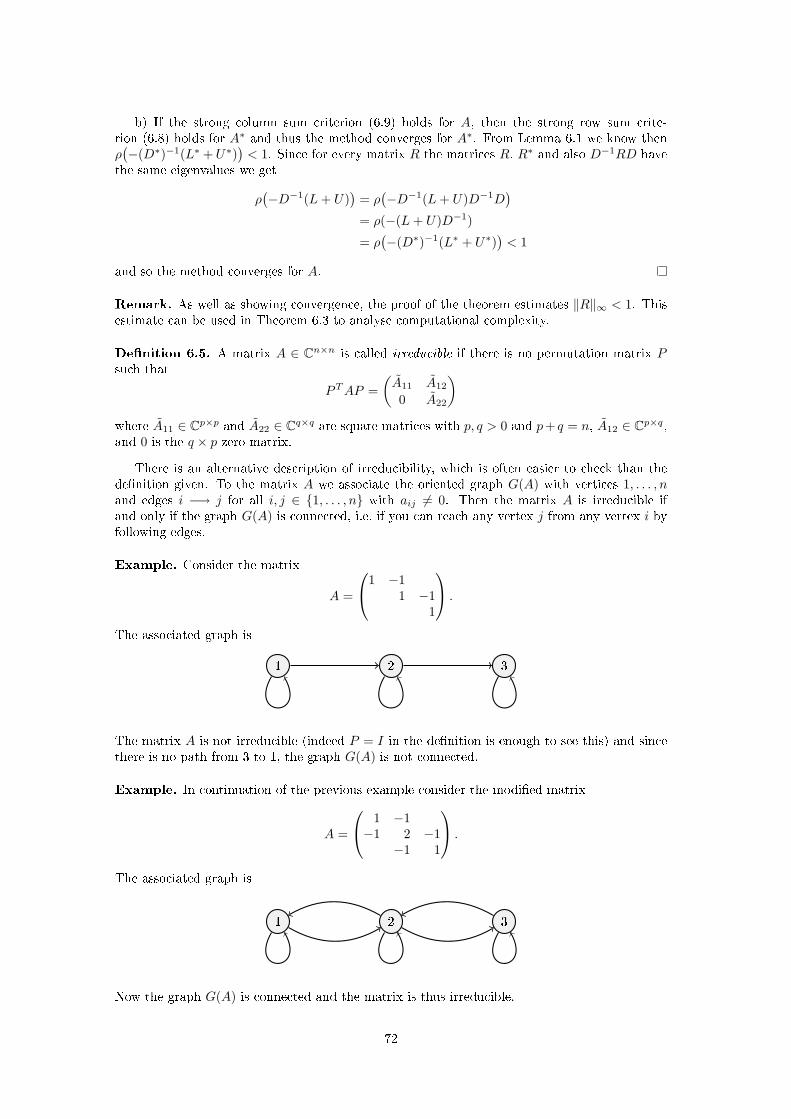
b) If the strong column sum criterion (6.9) holds for A, then the strong row sum crite-rion (6.8) holds for A∗ and thus the method converges for A∗. From Lemma 6.1 we know thenρ(−(D∗)−1(L∗ +U∗)
)< 1. Since for every matrix R the matrices R, R∗ and also D−1RD have
the same eigenvalues we get
ρ(−D−1(L+ U)
)= ρ(−D−1(L+ U)D−1D
)= ρ(−(L+ U)D−1)
= ρ(−(D∗)−1(L∗ + U∗)
)< 1
and so the method converges for A.
Remark. As well as showing convergence, the proof of the theorem estimates ‖R‖∞ < 1. Thisestimate can be used in Theorem 6.3 to analyse computational complexity.
Denition 6.5. A matrix A ∈ Cn×n is called irreducible if there is no permutation matrix Psuch that
PTAP =(A11 A12
0 A22
)where A11 ∈ Cp×p and A22 ∈ Cq×q are square matrices with p, q > 0 and p+ q = n, A12 ∈ Cp×q,and 0 is the q × p zero-matrix.
There is an alternative description of irreducibility, which is often easier to check than thedenition given. To the matrix A we associate the oriented graph G(A) with vertices 1, . . . , nand edges i −→ j for all i, j ∈ 1, . . . , n with aij 6= 0. Then the matrix A is irreducible ifand only if the graph G(A) is connected, i.e. if you can reach any vertex j from any vertex i byfollowing edges.
Example. Consider the matrix
A =
1 −11 −1
1
.
The associated graph is
1 2 3
The matrix A is not irreducible (indeed P = I in the denition is enough to see this) and sincethere is no path from 3 to 1, the graph G(A) is not connected.
Example. In continuation of the previous example consider the modied matrix
A =
1 −1−1 2 −1
−1 1
.
The associated graph is
1 2 3
Now the graph G(A) is connected and the matrix is thus irreducible.
72
Remarks.The proof of equivalence of the two characterisations of irreducibility is based on the following
observations.
1. For any permutation P the graphs G(A) and G(PTAP ) are isomorphic, only the verticesare numbered in a dierent way.
2. The block A22 in the denition of irreducibility corresponds to a set of states from wherethere is no path into the states corresponding to the block A11.
The characterisation of irreducibility through G(A) shows that the diagonal entries of A areirrelevant to determining irreducibility. Any matrix which has non-zero o-diagonal entries ifand only if A does so, will have the same graph. Hence R = −D−1(L+ U) is irreducible if andonly if A is.
Theorem 6.6. If A is irreducible and satises
|aii| ≥∑j 6=i
|aij | (6.10)
for i = 1, . . . , n but
|akk| >∑j 6=k
|akj | (6.11)
for one index k, then the Jacobi method converges. (This condition is called the weak row sumcriterion.)
Proof. We have to show that ρ(R) < 1 where R = −D−1(L + U). Dene the matrix |R| =(|rij |)ij ∈ Rn×n and the vector e = (1, 1, . . . , 1)T ∈ Rn. Then we have
(|R|e)i =( n∑j=1
|rij | · 1)i
=(∑j 6=i
|aij ||aii|
)≤ 1 = ei.
Thus |R|e ≤ e where this and some of the following inequalities between vectors are to be readcomponentwise. Therefore we get
|R|l+1e ≤ |R|le ≤ · · · ≤ e
for all l ∈ N.Let t(l) = e − |R|le ≥ 0. Then the vectors t(l) are componentwise increasing. Let τl be the
number of non-vanishing components of t(l). We will show that τl is strictly increasing until itreaches the value n. Assume, for contradiction, that τl+1 = τl = k < n. Since one row of Asatises the strict inequality (6.11) we have |R|e 6= e and thus k > 0. Then without loss ofgenerality (since we can reorder the rows and columns of A) we have
t(l) =(a0
), t(l+1) =
(b0
)where a, b ∈ Rk and a, b > 0. We can conclude(
b0
)= t(l+1) = e− |R|l+1e
≥ |R|e− |R|l+1e = |R|t(l)
=(|R11| |R12||R21| |R22|
)(a0
).
From a > 0 we have |R21| = 0. Hence R is not irreducible. This implies that A is not irreducible,and we have found the required contradiction. Thus we can conclude that τl+1 > τl wheneverτl < n. This proves t(n) > 0 componentwise.
Hence e > |R|ne and we get, using Lemma 1.34,
ρ(R)n ≤ ρ(Rn) ≤ ‖Rn‖∞ =∥∥|Rn|∥∥∞ ≤ ∥∥|R|n∥∥∞ = max
i=1,...,n
(|R|ne
)i< 1
and thus ρ(R) < 1. This completes the proof.
73

Computational Complexity
The sequence (xk)k∈N from the Jacobi method is dened by the relation
xk = −D−1(b− (L+ U)xk−1
).
For each iteration we have to calculate1) the product (L+ U)xk−1
2) the dierence b− · · · (needs n subtractions)3) the product D−1 · · · (needs n divisions because D is diagonal)
For general matrices the rst step needs Θ(n2) operations and thus dominates the computationalcost. If the matrix A is sparse, i.e. if it contains many zeros, the matrix-vector multiplicationcan be performed using fewer operations.
Example. Assume that each row of A contains at most ` > 0 non-zero entries outside thediagonal. Then step 1) requires Θ(n) operations and performing one step of Jacobi method hascost Θ(n) as n→∞. In this case we get α = 1 in Theorem 6.3.
6.3 The Gauss-Seidel and SOR Methods
The Method
The method obtained by usingM = L+ωD and N = U+(1−ω)D in (6.1), for the matrices L, Dand U from (6.7) and some ω ∈ R, is called the Successive Over Relaxation (SOR) scheme. Theparameter ω can be chosen to accelerate convergence. The special case ω = 1, i.e. M = L + Dand N = U , is called the Gauss-Seidel method. For the SOR scheme we get the iteration
(L+ ωD)xk = b− Uxk−1 − (1− ω)Dxk−1.
Since (L+ ωD) is lower triangular we can use forward substitution to calculate xk in each step.
Error Analysis
The error analysis of the SOR and Gauss-Seidel method is similar to the analysis for the Jacobimethod from the previous section. The convergence properties of the SOR scheme are determinedby the matrix
R = −(L+ ωD)−1(U + (1− ω)D
).
The following summarises some sucient criteria for convergence of the Gauss-Seidel method.
Theorem 6.7. Assume eithera) A satises the strong row sum criterion orb) A is irreducible and satises the weak row sum criterion.
Then the Gauss-Seidel (ω = 1) method converges.
Computational Complexity
The speed of convergence and thus the cost of the method depends on the choice of the param-eter ω. For linear systems arising from discretisation of certain elliptic PDEs, optimising canlead to an order of magnitude improvement in eciency, when compared with Gauss-Seidel andJacobi methods. This arises though decreasing β in Theorem 6.3 for appropriate choice of ω. Inthe same context Gauss-Seidel improves over Jacobi, but not by an order of magnitude.
74
6.4 Nonlinear Methods
In the remaining part of this chapter we will consider nonlinear methods for solving (SLE),i.e. methods where the map from xk to xk+1 is no longer linear. We restrict ourselves to thecase where the matrix A is Hermitian and positive denite. This section explains the generalapproach. The remaining two sections of the chapter examines two specic instances of nonlinearmethods in detail.
The fundamental observation for the methods we consider here is that the vector equationAx = b is equivalent to ‖Ax − b‖ = 0 for any vector norm ‖ · ‖. Since we assume that A isHermitian and positive denite, 〈x, y〉A = 〈x,Ay〉 denes an inner product and ‖x‖2A = 〈x,Ax〉denes the associated vector norm. The matrix A−1 is again Hermitian and positive deniteand ‖x‖2A−1 = 〈x,A−1x〉 denes the associated vector norm.
Lemma 6.8. Let A ∈ Cn×n be Hermitian and positive denite and b ∈ Cn. Then x ∈ Cn solvesAx = b if and only if x is the minimiser of the function
g(y) =12‖Ay − b‖2A−1 ∀y ∈ Cn. (6.12)
In this section we will consider iterative methods which solve (SLE) by constructing sequences(xk)k∈N which converge to the unique minimum of the function g. Using the residual rk = b−Axkand the error ek = x− xk, where x is the exact solution of Ax = b, we can write
g(xk) =12‖rk‖2A−1 =
12‖ek‖2A.
Thus minimising g corresponds to minimising the length of the residual vector in the ‖ · ‖A−1-norm or, equivalently, to minimising the error for the exact solution in the ‖ · ‖A-norm.
The Method
The two methods that we study below both take the form
xk = xk−1 + αk−1dk−1, (6.13)
where dk−1 ∈ Cn \ 0 is called the search direction and the scalar αk−1 ∈ C is called the steplength. The step length is chosen so that, given xk−1 and dk−1,
αk−1 = argminα∈C
g(xk−1 + αdk−1).
Since g is a convex, quadratic function, the value αk−1 is uniquely determined.The minimum can be found using the fact the g satises
g(y + εz) = g(y) + εRe〈z,Ay − b〉+ε2
2‖z‖2A (6.14)
for all ε ∈ R and y, z ∈ Cn, where Re denotes the real part of a complex number. Taking thederivative w.r.t. ε (along the real line) gives
∂
∂εg(y + εz)
∣∣ε=0
= Re〈z,Ay − b〉. (6.15)
At the minimum we nd
0 =∂
∂εg(xk−1 + αk−1dk−1 + εβdk−1)
∣∣ε=0
= Reβ〈dk−1, A(xk−1 + αk−1dk−1)− b〉= Reβ〈dk−1,−rk−1 + αk−1Adk−1〉
for all β ∈ C and thus
αk−1 =〈dk−1, rk−1〉‖dk−1‖2A
.
Hence we get the following algorithm.
75

Algorithm NI (nonlinear iterative methods).input: A ∈ Cn×n Hermitian and positive denite, b ∈ Cn, x0 ∈ Cnoutput: xk ∈ Cn with Axk ≈ b1: for k = 1, 2, 3, . . . do2: compute dk−1
3: αk−1 =〈dk−1, rk−1〉‖dk−1‖2A
4: xk = xk−1 + αk−1dk−1
5: end for
The steepest descent method and the conjugate gradient method, discussed below, are in-stances of this algorithm, employing dierent choices for the search directions dk.
Error Analysis
The error analysis for nonlinear methods is done in two steps. We rst study how fast thevalue ‖ek‖2A = 2g(xk) decays. This analysis depends on the specic choice of search directions dkand is presented for the two methods below, separately. In a second step we can use this resultto estimate the error of the approximate solution xk in the Euclidean norm:
Lemma 6.9. Assume ‖ek‖A ≤ cqk‖e0‖A for all k ∈ N for some constants q, c > 0. Then
‖ek‖ ≤√κ(A)c qk‖e0‖ ∀k ∈ N
where κ(A) = ‖A‖2‖A−1‖2 is the condition number of A in the 2-norm.
Proof. Let λmin and λmax be the minimal and maximal eigenvalue of A. Then we have κ(A) =λmax/λmin by (3.2) and from Lemma 1.21 we nd
‖ek‖2 ≤1
λmin‖ek‖2A ≤
2λmin
cqk‖e0‖2A ≤λmax
λmincqk‖e0‖2.
This completes the proof.
For future reference we state the following relation, which describes how the residual errorchanges in each step:
rk = rk−1 − αk−1Adk−1 ∀k ∈ N. (6.16)
This is a direct consequence of (6.13).
6.5 The Steepest Descent Method
The Method
The steepest descent method chooses a search direction which makes a step in the direction ofthe (locally) steepest descent for g. From equation (6.14) we get
g(xk + εdk) = g(xk)− εRe〈dk, rk〉+ε2
2‖dk‖2A (6.17)
for all ε ∈ R. Thus, the direction of steepest descent corresponds to the direction dk whichmaximises Re〈dk, rk〉 while keeping the length of dk xed. Since dk is only determined up to ascalar factor, we can choose
dk = rk ∀k ∈ N0
in (6.13). With this choice, the step length becomes
αk =‖rk‖2
‖rk‖2Aand we get the following algorithm.
76
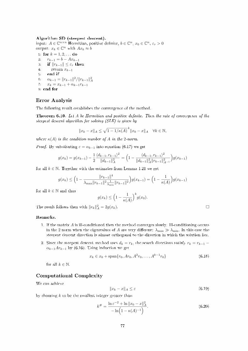
Algorithm SD (steepest descent).input: A ∈ Cn×n Hermitian, positive denite, b ∈ Cn, x0 ∈ Cn, εr > 0output: xk ∈ Cn with Axk ≈ b1: for k = 1, 2, . . . do2: rk−1 = b−Axk−1
3: if ‖rk−1‖ ≤ εr then4: return xk−1
5: end if6: αk−1 = ‖rk−1‖2/‖rk−1‖2A7: xk = xk−1 + αk−1rk−1
8: end for
Error Analysis
The following result establishes the convergence of the method.
Theorem 6.10. Let A be Hermitian and positive denite. Then the rate of convergence of thesteepest descent algorithm for solving (SLE) is given by
‖xk − x‖A ≤√
1− 1/κ(A)k‖x0 − x‖A ∀k ∈ N,
where κ(A) is the condition number of A in the 2-norm.
Proof. By substituting ε = αk−1 into equation (6.17) we get
g(xk) = g(xk−1)− 12〈dk−1, rk−1〉2
‖dk−1‖2A=(
1− 〈dk−1, rk−1〉2
‖dk−1‖2A‖rk−1‖2A−1
)g(xk−1)
for all k ∈ N. Together with the estimates from Lemma 1.21 we get
g(xk) ≤(
1− ‖rk−1‖4
λmax‖rk−1‖2 1λmin‖rk−1‖2
)g(xk−1) =
(1− 1
κ(A)
)g(xk−1)
for all k ∈ N and thus
g(xk) ≤(
1− 1κ(A)
)kg(x0).
The result follows then with ‖ek‖2A = 2g(xk).
Remarks.
1. If the matrix A is ill-conditioned then the method converges slowly. Ill-conditioning occursin the 2-norm when the eigenvalues of A are very dierent: λmax λmin. In this case thesteepest descent direction is almost orthogonal to the direction in which the solution lies.
2. Since the steepest descent method uses dk = rk, the search directions satisfy rk = rk−1 −αk−1Ark−1 by (6.16). Using induction we get
xk ∈ x0 + spanr0, Ar0, A2r0, . . . , A
k−1r0 (6.18)
for all k ∈ N.
Computational Complexity
We can achieve‖xk − x‖A ≤ ε (6.19)
by choosing k to be the smallest integer greater than
k# =ln ε−2 + ln ‖x0 − x‖2A− ln
(1− κ(A)−1
) . (6.20)
77

Assumption 6.11. 1. Calculation of Ax costs O(nα) uniformly in x ∈ Cn.
2. The condition number of A in the 2-norm satises κ(A) = O(nβ).
3. ‖x− x0‖A is bounded uniformly in n.
Theorem 6.12. Under Assumption 6.11 the computational cost of using the steepest descentmethod to achieve (6.19) is bounded above by cnmaxα,1+β ln ε−1, for some constant c indepen-dent of n and ε.
Proof. The rst item of the assumption ensures that each step of the iteration costs Θ(nmaxα,1).Hence, combining the second and third items and using (6.20) gives the desired result.
6.6 The Conjugate Gradient Method
Theorem 6.10 shows that the steepest descent method can behave quite poorly on ill-conditionedproblems. The conjugate gradient method, and its pre-conditioned variants, go a long way toameliorating this diculty, at little extra cost when compared to the method of steepest descents.
Again, we assume that A is Hermitian and positive denite. The conjugate gradient methodis similar to the steepest descent method but instead of making steps in direction of the steepestdescent it restricts the increments xk − xk−1 to lie in the Krylov subspace
Kk(A, r0) = spanr0, Ar0, A2r0, . . . , A
k−1r0.
Since the spaces Kk(A, r0) are increasing, this leads to xk ∈ x0 +Kk(A, r0) for all k and, as wewill see, the algorithm even chooses xk to minimise the function g from (6.12) on this space.
An underlying, general approach to the design of iterative methods for systems of linearequations (and also for the eigenvalue problem) is as follows: seek approximate solutions whichat the kth step of the iteration use only increments in Kk(A, r0). Such methods are natural whenmatrix-vector multiplication by A is cheap to compute. Equation (6.18) shows that the steepestdescent method follows this principle. The conjugate gradient method can be implemented al-most as easily as the method of steepest descents, but since it nds the optimal approximation tox from Kk(A, r0) we expect it to perform better. Indeed, the CG method converges considerablyfaster on ill-conditioned problems. Many other iterative methods also use the idea of ndingapproximations from the Krylov subspace.
The Method
Denition 6.13. Given A Hermitian positive-denite we say that the set d0, · · · , dk is A-orthogonal (or conjugate) if
〈di, dj〉A = 0 ∀i 6= j.
The following Lemma shows that choosing the search directions dk to be A-orthogonal isadvantageous for non-linear iterative methods.
Lemma 6.14. Assume that the search directions d0, . . . , dk−1 form an A-orthogonal set. Thenxk, given by (6.13), minimises g over x0 + spand0, · · · , dk−1.
Proof. Dene G : Cn → R by
G(γ) = g(x0 +k−1∑l=0
γldl) ∀γ ∈ Cn.
Then G is a convex quadratic function and has a unique minimum where all directional deriva-tives vanish. Using (6.15) with y = x0 +
∑k−1l=0 γldl and z = βdm we nd
Reβ〈dm, Ax0 +k−1∑l=0
γlAdl − b〉 = 0
78
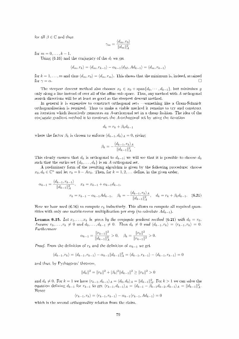
for all β ∈ C and thus
γm =〈dm, r0〉‖dm‖2A
for m = 0, . . . , k − 1.Using (6.16) and the conjugacy of the dl we get
〈dm, rk〉 = 〈dm, rk−1〉 − αk−1〈dM , Adk−1〉 = 〈dm, rk−1〉
for k = 1, . . . ,m and thus 〈dm, r0〉 = 〈dm, rm〉. This shows that the minimum is, indeed, attainedfor γ = α.
The steepest descent method also chooses xk ∈ x0 + spand0, · · · , dk−1, but minimises gonly along a line instead of over all of the ane sub-space. Thus, any method with A-orthogonalsearch directions will be at least as good as the steepest descent method.
In general it is expensive to construct orthogonal sets something like a Gram-Schmidtorthogonalisation is required. Thus to make a viable method it remains to try and constructan iteration which iteratively generates an A-orthogonal set in a cheap fashion. The idea of theconjugate gradient method is to construct the A-orthogonal set by using the iteration
dk = rk + βkdk−1
where the factor βk is chosen to enforce 〈dk−1, dk〉A = 0, giving
βk = −〈dk−1, rk〉A‖dk−1‖2A
.
This clearly ensures that dk is orthogonal to dk−1; we will see that it is possible to choose d0
such that the entire set d0, . . . , dk is an A-orthogonal set.A preliminary form of the resulting algorithm is given by the following procedure: choose
x0, d0 ∈ Cn and let r0 = b−Ax0. Then, for k = 1, 2, . . . dene, in the given order,
αk−1 =〈dk−1, rk−1〉‖dk−1‖2A
, xk = xk−1 + αk−1dk−1,
rk = rk−1 − αk−1Adk−1, βk = −〈dk−1, rk〉A‖dk−1‖2A
, dk = rk + βkdk−1. (6.21)
Here we have used (6.16) to compute rk inductively. This allows to compute all required quan-tities with only one matrix-vector multiplication per step (to calculate Adk−1).
Lemma 6.15. Let x1, . . . , xk be given by the conjugate gradient method (6.21) with d0 = r0.Assume r0, . . . , rk 6= 0 and d0, . . . , dk−1 6= 0. Then dk 6= 0 and 〈dk−1, rk〉 = 〈rk−1, rk〉 = 0.Furthermore
αk−1 =‖rk−1‖2
‖dk−1‖2A> 0, βk =
‖rk‖2
‖rk−1‖2> 0.
Proof. From the denition of rk and the denition of αk−1 we get
〈dk−1, rk〉 = 〈dk−1, rk−1〉 − αk−1‖dk−1‖2A = 〈dk−1, rk−1〉 − 〈dk−1, rk−1〉 = 0
and thus, by Pythagoras' theorem,
‖dk‖2 = ‖rk‖2 + |βk|2‖dk−1‖2 ≥ ‖rk‖2 > 0
and dk 6= 0. For k = 1 we have 〈rk−1, dk−1〉A = 〈d0, d0〉A = ‖dk−1‖2A. For k > 1 we can solve theequation dening dk−1 for rk−1 to get 〈rk−1, dk−1〉A = 〈dk−1 − βk−1dk−2, dk−1〉A = ‖dk−1‖2A.Hence
〈rk−1, rk〉 = 〈rk−1, rk−1〉 − αk−1〈rk−1, Adk−1〉 = 0
which is the second orthogonality relation from the claim.
79
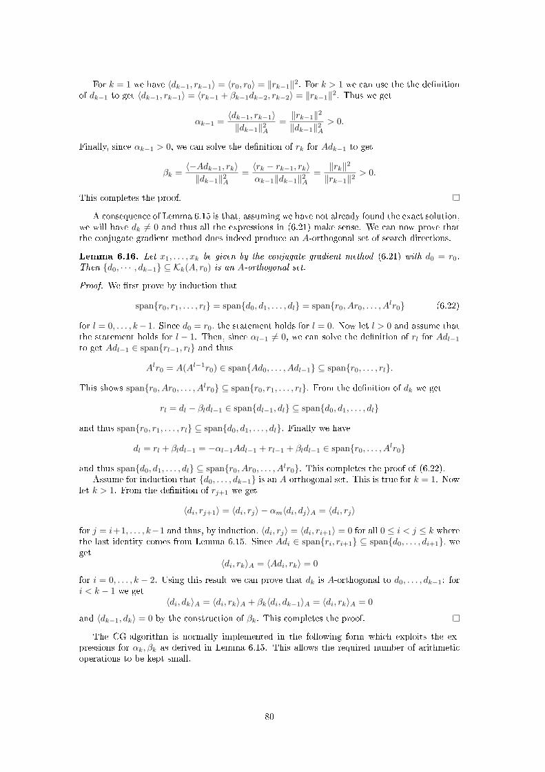
For k = 1 we have 〈dk−1, rk−1〉 = 〈r0, r0〉 = ‖rk−1‖2. For k > 1 we can use the the denitionof dk−1 to get 〈dk−1, rk−1〉 = 〈rk−1 + βk−1dk−2, rk−2〉 = ‖rk−1‖2. Thus we get
αk−1 =〈dk−1, rk−1〉‖dk−1‖2A
=‖rk−1‖2
‖dk−1‖2A> 0.
Finally, since αk−1 > 0, we can solve the denition of rk for Adk−1 to get
βk =〈−Adk−1, rk〉‖dk−1‖2A
=〈rk − rk−1, rk〉αk−1‖dk−1‖2A
=‖rk‖2
‖rk−1‖2> 0.
This completes the proof.
A consequence of Lemma 6.15 is that, assuming we have not already found the exact solution,we will have dk 6= 0 and thus all the expressions in (6.21) make sense. We can now prove thatthe conjugate gradient method does indeed produce an A-orthogonal set of search directions.
Lemma 6.16. Let x1, . . . , xk be given by the conjugate gradient method (6.21) with d0 = r0.Then d0, · · · , dk−1 ⊆ Kk(A, r0) is an A-orthogonal set.
Proof. We rst prove by induction that
spanr0, r1, . . . , rl = spand0, d1, . . . , dl = spanr0, Ar0, . . . , Alr0 (6.22)
for l = 0, . . . , k− 1. Since d0 = r0, the statement holds for l = 0. Now let l > 0 and assume thatthe statement holds for l − 1. Then, since αl−1 6= 0, we can solve the denition of rl for Adl−1
to get Adl−1 ∈ spanrl−1, rl and thus
Alr0 = A(Al−1r0) ∈ spanAd0, . . . , Adl−1 ⊆ spanr0, . . . , rl.
This shows spanr0, Ar0, . . . , Alr0 ⊆ spanr0, r1, . . . , rl. From the denition of dk we get
rl = dl − βldl−1 ∈ spandl−1, dl ⊆ spand0, d1, . . . , dl
and thus spanr0, r1, . . . , rl ⊆ spand0, d1, . . . , dl. Finally we have
dl = rl + βldl−1 = −αl−1Adl−1 + rl−1 + βldl−1 ∈ spanr0, . . . , Alr0
and thus spand0, d1, . . . , dl ⊆ spanr0, Ar0, . . . , Alr0. This completes the proof of (6.22).
Assume for induction that d0, . . . , dk−1 is an A-orthogonal set. This is true for k = 1. Nowlet k > 1. From the denition of rj+1 we get
〈di, rj+1〉 = 〈di, rj〉 − αm〈di, dj〉A = 〈di, rj〉
for j = i+1, . . . , k−1 and thus, by induction, 〈di, rj〉 = 〈di, ri+1〉 = 0 for all 0 ≤ i < j ≤ k wherethe last identity comes from Lemma 6.15. Since Adi ∈ spanri, ri+1 ⊆ spand0, . . . , di+1, weget
〈di, rk〉A = 〈Adi, rk〉 = 0
for i = 0, . . . , k − 2. Using this result we can prove that dk is A-orthogonal to d0, . . . , dk−1: fori < k − 1 we get
〈di, dk〉A = 〈di, rk〉A + βk〈di, dk−1〉A = 〈di, rk〉A = 0
and 〈dk−1, dk〉 = 0 by the construction of βk. This completes the proof.
The CG-algorithm is normally implemented in the following form which exploits the ex-pressions for αk, βk as derived in Lemma 6.15. This allows the required number of arithmeticoperations to be kept small.
80
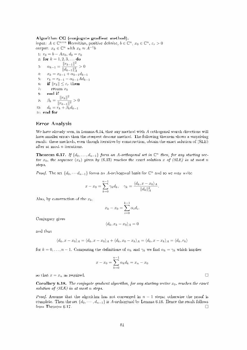
Algorithm CG (conjugate gradient method).input: A ∈ Cn×n Hermitian, positive denite, b ∈ Cn, x0 ∈ Cn, εr > 0output: xk ∈ Cn with xk ≈ A−1b
1: r0 = b−Ax0, d0 = r0
2: for k = 1, 2, 3, . . . do
3: αk−1 =‖rk−1‖2
‖dk−1‖2A> 0
4: xk = xk−1 + αk−1dk−1
5: rk = rk−1 − αk−1Adk−1
6: if ‖rk‖ ≤ εr then7: return xk8: end if
9: βk =‖rk‖2
‖rk−1‖2> 0
10: dk = rk + βkdk−1
11: end for
Error Analysis
We have already seen, in Lemma 6.14, that any method with A-orthogonal search directions willhave smaller errors than the steepest descent method. The following theorem shows a surprisingresult: these methods, even though iterative by construction, obtain the exact solution of (SLE)after at most n iterations.
Theorem 6.17. If d0, . . . , dn−1 form an A-orthogonal set in Cn then, for any starting vec-tor x0, the sequence (xk) given by (6.13) reaches the exact solution x of (SLE) in at most nsteps.
Proof. The set d0, · · · dn−1 forms an A-orthogonal basis for Cn and so we may write
x− x0 =n−1∑k=0
γkdk, γk =〈dk, x− x0〉A‖dk‖2A
.
Also, by construction of the xk,
xk − x0 =k−1∑i=0
αidi.
Conjugacy gives〈dk, xk − x0〉A = 0
and thus
〈dk, x− x0〉A = 〈dk, x− x0〉A + 〈dk, x0 − xk〉A = 〈dk, x− xk〉A = 〈dk, rk〉
for k = 0, . . . , n− 1. Comparing the denitions of αk and γk we nd αk = γk which implies
x− x0 =n−1∑k=0
αkdk = xn − x0
so that x = xn as required.
Corollary 6.18. The conjugate gradient algorithm, for any starting vector x0, reaches the exactsolution of (SLE) in at most n steps.
Proof. Assume that the algorithm has not converged in n − 1 steps; otherwise the proof iscomplete. Then the set d0, · · · , dn−1 is A-orthogonal by Lemma 6.16. Hence the result followsfrom Theorem 6.17.
81

Remark. When the computation is performed on a computer, rounding errors will cause rn 6= 0where rn is the calculated value for the residual error rn. In practice one just treats the methodas an iterative method and continues the iteration until the residual error ‖rk‖ is small enough.Typically the exit criterion will even be reached for k < n.
In order to understand how the conjugate gradient method performs iteratively, we describean error analysis based around the theory of polynomial approximation. In the following we let
Λ(A) := λ ∈ C | λ is an eigenvalue of A
and we let Pk denote the set of all polynomials of degree k with p(0) = 1.
Theorem 6.19. If the conjugate gradient algorithm has not converged at step k, then
‖xk − x‖A = infp∈Pk
‖p(A)(x0 − x)‖A
≤(
infp∈Pk
maxλ∈Λ(A)
|p(λ)|)‖x0 − x‖A.
Proof. Since xk ∈ x0 + spanr0, Ar0, . . . , Ak−1r0 we can nd γj ∈ C with
ek = x− xk = x− x0 +k−1∑j=0
γjAjr0 = e0 +
k−1∑j=0
γjAj+1e0.
Dening p ∈ Pk by
p(λ) = 1 +k∑j=1
γj−1λj
we obtain ek = p(A)e0 and thus
‖xk − x‖A = ‖p(A)(x0 − x)‖A.
The value xk minimises ‖xk − x‖A over xk ∈ Kk(A, b), which is equivalent to minimising overall choices of γj . Hence
‖xk − x‖A = infp∈Pk
‖p(A)(x0 − x)‖A.
To complete the proof let (ψj) be a basis of Cn composed of eigenvectors of A with corre-sponding eigenvalues λj . If we let e0 =
∑nj=1 ajψj , then
ek = p(A)e0 =n∑j=1
ajp(λj)ψj
and thus we get
‖e0‖2A =n∑j=1
λj |aj |2, ‖ek‖2A =n∑j=1
λj |ajp(λj)|2.
Therefore
‖ek‖2A ≤ maxλ∈Λ(A)
|p(λ)|2n∑j=1
|aj |2λj = maxλ∈Λ(A)
|p(λ)|2‖e0‖2A
and the result follows.
By choosing an appropriately scaled and shifted Chebyshev polynomial and applying theprevious result, the following may be shown:
Theorem 6.20. Let κ be the condition number of a symmetric positive denite matrix A in theEuclidean norm. Then the error in step k of the conjugate gradient algorithm for solving (SLE)satises
‖xk − x‖A ≤ 2
[(√κ+ 1√κ− 1
)k+(√
κ+ 1√κ− 1
)−k]−1
‖x0 − x‖A.
Proof. See Exercise 6-6.
82

Computational Complexity
We make the same assumptions as for the steepest descent method, and show the decrease incomputational cost that can be obtained by using the conjugate gradient method.
Theorem 6.21. Under Assumption 6.11 the computational cost of using the conjugate gra-dient method to achieve (6.19) is bounded above by cnmaxα,1+ 1
2β ln ε−1, for some constant cindependent of n and ε.
Proof. The rst item of the assumption ensures that each step of the iteration costs Θ(nmaxα,1).If√κ 1 then the Theorem 6.20 gives
‖xk − x‖A . 2(
1− 2√κ
)k‖x0 − x‖A.
Combining the second and third items and using this expression gives the desired result.
Remark. In an applied context the most important form of the conjugate gradient method isits preconditioned form. Roughly speaking the method is applied to the linear system
MAx = Mb
where the preconditioner M is chosen to try and improve the conditioning of MA over A, yethaveM easy to invert. In practical terms the algorithm diers from standard conjugate gradientonly by the addition of one multiplication with M per step.
Bibliography
Linear iterative methods for (SLE) are described in the book [Saa97]. Theorem 6.7 is proved in[SB02]. For discussion of Theorem 6.20 see [TB97]; for related results see [NW06]. The SORmethod is analysed in detail in [LT88].
The nonlinear iterative methods that we discuss are constructed through minimisation oroptimisation techniques. As such they are strongly related to the topic of optimisation in general.This topic is well overviewed in [NW06]; the exposition of the conjugate gradient method thereforms the basis for ours. A good discussion of preconditioned versions of the conjugate gradientmethod may also be found in this book.
Exercises
Exercise 6-1. The purpose of this exercise is to introduce you to the idea of iteration. Manyproblems are simply too large to solve by the methods we have looked at so far too muchcomputer time or memory is required if the dimension n of the matrix is large. For linear systems
Ax = b, A ∈ Rn×n, b ∈ Rn (6.23)
this will lead to the idea of generating approximating sequences xk which hopefully convergeto x as k →∞. For eigenvalue problems which are large we will study methods which generateapproximations to a subset of the eigenvalues, and not to all of them. (Note that for eigenvalueproblems it is necessary to use iterative methods in all cases, provided the matrix has dimensionbigger than 4; the main dierence when the problem is large is that we solve for only a subsetof the eigenvalues).(i) To show why iterative methods are necessary construct a matrix A with n = 1000 as follows:type
>> A=0.0005*rand(1000);
>> b=rand(1000,1);
>> for i=1:1000; A(i,i)=1; end;
83
This creates a matrix A with 1 on the diagonal and random entries uniformly distributed in[0, 5× 10⁻⁴] on the o-diagonals. Now try solving (6.23). Type
>> x=A\b;
Almost certainly your computer cannot handle a problem of this size. So type ctrl c to stop itfrom trying. (If you are lucky enough to be working on a machine where this problem is solvedeasily then repeat the exercise replacing 1000 by 10000 or by some matrix suciently large thatMatlab fails.) Keep the (original 1000 × 1000) matrix A for use in (iii) where we will use amore successful approach to solve this problem.(ii) We look at the simplest iterative method, known as Jacobi. Any matrix A can be writtenuniquely as
A = D + L+ U
whereD is diagonal, L is zero on and above the diagonal and U is zero on and below the diagonal.Assuming that D is invertible, consider a sequence xk∞k=1 satisfying
xk+1 = D−1[b− Lxk − Uxk].
If xk → x∗ as k →∞ then what equation does x∗ satisfy and why?(iii) Implement the idea in (ii) as follows. Type
>> L=tril(A,-1);
>> U=triu(A,1);
>> 0=L+U;
This creates L and U as dened in (ii) (a Matlab question: why is this so?). Type
>> j=1;
>> y=ones(1000,1);
>> n(j)=2*j;
>> for i=1:n(j); y=b-O*y; end
>> rn(j)=norm(A*y-b)
What does this tell you? Repeat the above 5 lines of code with j = 2, 3, . . . , 5 and type:
>> plot(n,rn)
What do you observe? Also type
>> plot(n,log(rn))
(iv) Under what conditions on A will the Jacobi iteration converge to the correct solution of(6.23)?
Exercise 6-2. Prove that the Jacobi iteration that you implemented in Exercise 6-1 convergesfor the matrix A given there.
Exercise 6-3. Which of the following matrices are irreducible? For which of these matricesdoes the Jacobi-method converge?4 2 1
2 11
,
1 33 25 4
4 1
,
84 22 1 1
Exercise 6-4. Show that the Jacobi method for the solution of1 1
1 10 22 1
x1
x2
x3
=
123
converges and, for the iteration starting with x0 = 0, give an upper bound on the number ofsteps required to get the relative error of the result below 10−6.
84
Exercise 6-5. Consider the linear system Ax = b where
A =(
1 00 ε
),
where b = (1, ε)T . Calculate x1 from the steepest descents algorithm, starting from x0 = 0.Which component of the solution is better approximated after one step? Why is this?
Exercise 6-6. Prove Theorem 6.20 by choosing a Chebyshev polynomial scaled and shifted sothat its min/max properties hold on the interval [λmin(A), λmax(A)]. Then prove that
‖xk − x‖A ≤ 2δk‖x0 − x‖A
where δ ∈ (0, 1) and
δ ≈ 1− 2√µmin
µmax
for κ 1.
Exercise 6-7. Let A ∈ Rn×n be a symmetric positive-denite matrix. If A = QMQT is theeigenvalue/eigenvector decomposition of A, then we dene a square root of A (one of manypossible square roots) to be A1/2 = QDQT , where D is a diagonal matrix whose elements arethe square roots of the corresponding elements of M .
1. If B ∈ Rn×n is a matrix such that B and A1/2 commute, prove that
‖Bx‖A ≤ ‖B‖2‖x‖A, ∀x ∈ Rn
2. Using your proof above, prove that
infp∈Pk
‖p(A)y‖A ≤ infp∈Pk
maxλ∈Λ(A)
|p(λ)|‖y‖A
where Pk is the set of all polynomials p of degree less than or equal to k with p(0) = 1,y ∈ Rn, and Λ(A) is the set of eigenvalues of A.
Exercise 6-8. Dene
ϕ(x) :=12〈x,Ax〉 − 〈x, b〉
with A symmetric positive denite. Show that minimising ϕ(x) is equivalent to solving Ax = b.Consider the algorithm
xk+1 = xk + αkrk
to minimise ϕ(x). Find αk which minimises ϕ(xk+1) over all αk ∈ R given xk. This choice ofαk denes the gradient or steepest descent algorithm.
For CG we havexk+1 = xk + αkdk.
Show that the choice of αk made in Algorithm CG minimises ϕ(xk+1) over all α ∈ R, given xkand dk.
85
Chapter 7
Least Squares Problems
In this chapter we introduce algorithms for the (LSQ) problem: given A ∈ Cm×n and b ∈ Cmwith m ≥ n, nd x ∈ Cn which minimises ‖Ax−b‖2. We will describe and discuss three dierentalgorithms to solve (LSQ). The following theorem underpins all of the algorithms described.
Theorem 7.1. A vector x ∈ Cn minimises ‖Ax − b‖2 for A ∈ Cm×n and b ∈ Cm, if and onlyif Ax− b is orthogonal to range(A).
Proof. Let g(x) = 12‖Ax − b‖ 2
2 . Then minimising ‖Ax − b‖2 is equivalent to minimising thefunction g.
Assume that Ax− b is orthogonal to range(A) and let y ∈ Cn. Then
Ay −Ax = A(y − x) ⊥ Ax− b
and Pythagoras' theorem gives
‖Ay − b‖ 22 = ‖Ay −Ax‖ 2
2 + ‖Ax− b‖ 22 ≥ ‖Ax− b‖ 2
2
for all y ∈ Cn. Thus x minimises g.Now assume that the vector x minimises g. Then for every y ∈ Cn we have
0 =∂
∂λg(x+ λy) =
12
(〈Ay,Ax− b〉+ 〈Ax− b, Ay〉
)= Re〈Ax− b, Ay〉
and
0 =∂
∂λg(x+ λiy) =
12
(−i〈Ay,Ax− b〉+ i〈Ax− b, Ay〉
)= − Im〈Ax− b, Ay〉.
This shows 〈Ax− b, Ay〉 = 0 and thus Ax− b ⊥ Ay for all y ∈ Cn.
Corollary 7.2. A vector x ∈ Cn solves (LSQ) if and only if
A∗Ax = A∗b. (7.1)
Proof. From the theorem we know that x solves (LSQ) if and only if Ax − b ⊥ range(A). Thisin turn is equivalent to Ax− b ⊥ ai for every column ai of A, i.e. to A
∗(Ax− b) = 0.
It is hence of interest to know whether A∗A is invertible. We assume throughout the remain-der of this chapter that the singular values of A satisfy
σ1 ≥ σ2 ≥ · · · ≥ σn > 0
and in this case A∗A is indeed invertible. Under this assumption, (LSQ) is solved by
x = A†b
where the pseudo-inverse A† = (A∗A)−1A∗ is dened in Denition 3.6. The system (7.1) iscalled the normal equations for (LSQ).
Recall the denition of the 2-norm condition number for (LSQ) from Chapter 3. Note thatthis is large when A is close to being rank-decient, so that σn is small. In many practicalapplications of (LSQ), such as arise naturally in statistics, A is indeed close to being rank-decient. We will comment on this issue when we discuss the stability of the algorithms.
86
7.1 LSQ via Normal Equations
The Method
A natural approach to solution of the normal equations is as follows:
Algorithm (LSQ via normal equations).input: A ∈ Cm×n with m ≥ n and rank(A) = n, b ∈ Cmoutput: x ∈ Cn with minimal ‖Ax− b‖21: calculate A∗A and A∗b2: solve (A∗A)x = A∗b
Computational Complexity
The method is usually implemented via standard algorithms for the matrix-matrix multiplica-tion and matrix-vector multiplication, together with Cholesky factorisation for solution of thesymmetric linear system.
Theorem 7.3 (Cost of Normal Equations for LSQ). The cost of solving (LSQ) by the NormalEquations approach is, in the usual implementation described above,
C(m,n) ∼ mn2 +13n3
as m,n→∞.
Proof. Calculating A∗A and A∗b requires asymptotically ∼ 2mn2 operations for m,n → ∞.Since A∗A is symmetric we only need to calculate half of the entries, which can be done in∼ mn2 operations. Calculation of A∗b costs Θ(mn). Solving (A∗A)x = A∗b with Cholesky-factorisation requires ∼ 1
3n3 operations. Combining these terms gives the result.
Of particular interest is the case m ∼ an as n → ∞ for some constant a 1, which arisesfrequently in practice. If a 1 the cost is dominated by mn2.
Error Analysis
One way that the error analysis proceeds is by proving that the computed x, x, solves
(A∗A+ ∆A)x = A∗b+ c
and then using the backward error analysis for (SLE). Because κ(A∗A) = κ(A)2 in the 2-normit follows that
‖∆x‖2‖x‖2
= O(κ(A)2εm
).
In practice this method can perform very badly when the matrix A is close to being rank-decient(so that σn is small by Lemma 3.8) and the 2-norm condition number of A is large.
7.2 LSQ via QR factorisation
The Method
To increase stability, at an increase in computational cost, the following QR based algorithm isoften used in practice.
Algorithm (LSQ via QR factorisation).input: A ∈ Cm×n with m ≥ n and rank(A) = n, b ∈ Cmoutput: x ∈ Cn with minimal ‖Ax− b‖21: compute the reduced QR factorisation A = QR2: compute Q∗b ∈ Cn3: solve Rx = Q∗b using back substitution
87
The result of the algorithm satises
A∗Ax = A∗QRx
= A∗QQ∗b
= R∗Q∗QQ∗b
= R∗Q∗b
= A∗b
and thus solves (LSQ).
Computational Complexity
The method is usually implemented by means of Householder based QR factorisation, standardmatrix-vector multiplication for Q∗b and standard triangular inversion of R. As for the normalequations approach, we assume that there is positive a, independent of n, such that m ∼ an asn→∞.
Theorem 7.4 (Cost of QR for LSQ). Let sn(A) > 0. The cost of solving (LSQ) by the QRapproach is, in the usual implementation,
2mn2 − 23n3 + Θ(mn+ n2).
Proof. Steps 1 and 2 together have asymptotic cost C1(m,n) ∼ 2mn2− 23n
3 +Θ(mn), and step 3has asymptotic cost C2(m,n) = Θ(n2). Thus we get the desired result.
If a 1 then the cost is dominated by 2mn2 and is roughly twice that of the normal equationsapproach.
Error Analysis
The Householder QR approach has considerably improved backward stability properties whencompared with the normal equations based solution method. In particular, the backward erroris small in the following sense.
Theorem 7.5. Let x solve the (LSQ) problem for (A, b) and let x be the computer solution viaHouseholder QR factorisation. Then x minimises ‖(A+ ∆A)x− (b+ ∆b)‖2 for matrix ∆A withcolumns ∆aj and vector ∆b satisfying, for εm suciently small,
‖∆aj‖2 ≤Cmnεm
1− Cmnεm‖aj‖2, j = 1, . . . , n
‖∆b‖2 ≤Cmnεm
1− Cmnεm‖b‖2.
In contrast to the normal equations method, this bound on the backward error is independentof the condition number of A. However, practitioners are often interested in the implied error inestimating the residual r = b−Ax. This can still behave poorly for the QR method, particularlywhen the matrix A is ill-conditioned.
7.3 LSQ via SVD
The Method
The most stable solution of (LSQ), especially useful for problems where A is close to beingrank-decient, and σn close to zero, is SVD based.
88
Algorithm (LSQ via SVD).input: A ∈ Cm×n with m ≥ n and rank(A) = n, b ∈ Cmoutput: x ∈ Cn with minimal ‖Ax− b‖21: compute the reduced SVD A = U ΣV ∗
2: compute U∗b ∈ Cn3: solve Σy = U∗b4: return x = V y
The result x of the calculation satises
A∗Ax = A∗U ΣV ∗V y = A∗U U∗b = A∗b
and thus it is the solution of (LSQ).
Computing the SVD
Assume that we are given A ∈ Cm×n. A common approach to computing the SVD is as follows:
• Step 1. Find the reduced QR factorisation A = QR with Q ∈ Cm×n and R ∈ Cn×n.
• Step 2. Perform a bidiagonalisation of R, via orthogonal transformations as in Lemma 4.11,so that B = U∗1RV1 where B ∈ Cn×n is upper-bidiagonal: has non-zeros only on thediagonal and on the rst upper o-diagonal.
• Step 3. Find an SVD B = U2ΣV ∗2 by use of Theorem 2.17.
• Step 4. Note that A = (QU1U2)Σ(V1V2)∗ and that hence A = UΣV ∗ with orthogonal U, Vgiven by U = QU1U2, V = V1V2. (Note that the composition of orthogonal matrices isitself orthogonal).
It may be shown that the cost of this algorithm is 2mn2 + 11n3 + Θ(mn+ n2).
Computational Complexity
Using these ideas is the basis for the standard implementation of SVD based approaches to(LSQ). As for the normal equations approach, we assume that there is a positive a, independentof n, such that m ∼ an as n→∞.
Theorem 7.6 (Cost of SVD for LSQ). Let sn(A) > 0. The cost of solving (LSQ) by the SVDapproach is, in the usual implementation,
2mn2 + 11n3 + Θ(mn+ n2).
Proof. (Sketch) SVD is 2mn2 + 11n3 + Θ(mn+ n2).
form c = U∗b : Θ(mn)
solve Σw = c : Θ(n)
form x = V y : Θ(n2).
If a 1 the cost is similar to that of of the QR based method. But, for moderate valuesof a, the additional 11n3 term means that this method can be considerably more time-consumingthan the QR method.
Error Analysis
The SVD approach is by far the most stable of the three methods for (LSQ). This is becauseit reveals the singular values which are close to zero, and hence possibly reect rank-deciencyof A. Exploiting this fact, enables the method to perform well even in situations which are closeto rank-decient and, in particular, where σn is very close to zero.
89
Bibliography
The books [TB97] and [Dem97] both contain clear discussions of algorithms for (LSQ); thestatements about complexity of the SVD, and SVD based methods for (LSQ) may be found in[TB97] for example. More details concerning the error analysis, and Theorem 7.5 in particular,can be found in [Hig02].
Exercises
Exercise 7-1. The purpose of this question is to introduce you to the content of this chapter.It is broken into three parts: (i) formulate a least squares problem; (ii) solve it blindly usingMatlab; (iii) introduce the SVD, a major tool used in solving least squares problems.(i) Let (u(i), v(i))mi=1 be a set of points in the (u, v) plane. We wish to nd the best straightline t
v = αu+ β
to this data. The least squares approach to this problem is to nd (α, β) ∈ R2 minimising
G(α, β) =m∑i=1
|αu(i) + β − v(i)|2.
Show that G may be written asG(α, β) = ‖Ay − b‖22
for y = (α, β)T and some choice of A ∈ Rm×2 and b ∈ Rm which you should specify.(ii) Generate some data (u(i), v(i))100
i=1 in the following way: specify some delta ∈ R and type
>> u=rand(100,1);
>> v=2*u+ones(100,1)+delta*rand(100,1);
Construct A and b as dened in (i) and then form
>> x=A\b
This is the least squares solution. What would you expect the solution to be if delta is verysmall? Test your hypothesis by repeating the previous construction of A and b for a variety ofsmall delta.(iii) As we shall see, there are several competing methods to solve a least squares problem. Oneis based on the QR decomposition. A second is based on the SVD (singular value decomposi-tion). To make the matrices shorter type A=A(1:5,:). We will perform operations on this newshortened version of A (corresponding to 5 data points rather than 100.) Type
>> [U,X,V]=svd(A)
and discuss the properties of U , X and V (think about columns!). Now type
>> rn=norm(U*X*V'-A)
What does this tell you? Now type
>> [W,S,Z]=svd(A,0)
and compare W,S and Z with U,X and V . Again type
>> rn=norm(W*S*Z'-A)
What does this tell you?The two factorisations are known (respectively) as the full SVD and the reduced SVD In our
theoretical development we will mainly use the reduced SVD, and will refer to this as the SVDfor short.
90
Exercise 7-2. You are given m data points (u(i), v(i)) where u(i) ∈ Rn−1 and v(i) ∈ R fori = 1, . . . ,m. We would like to nd α ∈ Rn−1 and β ∈ R to minimise
m∑i=1
|αTu(i) + β − v(i)|2.
Show that this problem may be reformulated as a standard least squares problem by specifyingappropriate choices of A ∈ Rm×n and b ∈ Rm.
Now let n = 2 and generate m = 50 random data points of the form
v(i) = u(i) + 10−2W (i)
where the u(i) are chosen at random uniformly from [0, 100] and the W (i) are chosen at randomfrom the standard normal distribution (with mean zero and variance one). Solve the resultingleast squares problem by the QR method and by using the SVD (make use of Matlab's qr andsvd routines). What do you expect the answer to be? Compare the eciency and accuracy ofthe two dierent methods.
Exercise 7-3. Vandermonde matrices again: remember the command vander in Matlab.a) Consider the polynomial interpolation problem. For each of the cases l = 2, 4, 6, 8, 10,
generate a square Vandermonde matrix B(l) with the data points ujlj=1 chosen from the set
1, 2, . . . , l. Estimate the condition numbers of the B(l) with the Matlab routine cond, and plotit as a function of l. What do you deduce from this exercise?
b) Now consider the problem of polynomial data tting. Write down a least squares problemBα = v which determines the coecients αjnj=1 in a polynomial
v(x) =n∑j=1
αjuj
which best ts the data points (uj , vj)nj=1 in the sense of minimising
m∑i=1
|v(ui)− vi|2.
The matrix B is a rectangular Vandermonde matrix. For each of the cases l = 2, 4, 6, 8, 10,generate the rectangular B(l) with m = l and n = l/2. Choose the data points ujlj=1 from the
set 1, 2, . . . , l. Estimate the condition numbers of the B(l) with the Matlab routine cond, andplot it as a function of l. Discuss what you observe in relation to the rst part of the question.
c) Now consider the data points
uj = j, j = 1, . . . , 9u10 = 9.0000001
vj = 1 + uj + u4j + 10−2W (j)
where the W (j) are independently chosen at random from the standard normal distribution(mean zero and variance one). Find the tenth degree polynomial interpolant to this data set,using QR factorisation. Then nd the best t polynomial of degree four, using QR to solve theresulting least squares problem. Compare the results you obtain from interpolation and best t.Use graphical output to illustrate your discussion.
Exercise 7-4. Let A ∈ Rn×n be symmetric positive denite with eigenvalues
0 < µ1 ≤ µ2 ≤ . . . ≤ µn.
1. Show that‖A‖2 = µn and ‖A−1‖2 = µ−1
1 .
What is the condition number of A in the Euclidean norm in this case?
91
2. Explicitly nd δA solving
min‖δA‖2‖A‖2
: A+ δA is singular
.
How big is ‖δA‖2/‖A‖2 for this δA?
3. Let B ∈ Rm×n with m > n. State and derive the normal equations for the solution of theleast squares problem
minx∈Rn
‖Bx− b‖2
where b ∈ Rm.
4. If B has singular values σini=1 then what is the Euclidean norm condition number of thematrix which must be inverted to solve the normal equations?
Exercise 7-5. Show that the least squares solution will yield Ax = b if and only if b = AA†bwhere A† is the Moore-Penrose inverse of A.
92
Chapter 8
Eigenvalue Problems
In this chapter we will study methods for solution of the eigenvalue problem (EVP): givenA ∈ Cn×n, compute the eigenvalues and eigenvectors of A.
A rst insight is that nding eigenvalues and nding eigenvectors are equivalent problems.To nd an eigenvalue from an eigenvector we proceed as follows: Given an eigenvector x ∈ Cn wetry to nd the α ∈ C which minimises ‖αx−Ax‖2. Since x is an eigenvector, the minimum of 0is attained for the corresponding eigenvalue. It is easy to check, for example using Corollary 7.2,that the optimal choice of α is
α = (x∗x)−1x∗(Ax) =〈x,Ax〉〈x, x〉
.
Note that solvability of the normal equations in this case is guaranteed, provided that x 6= 0. Thepreceding considerations show that the following denition provides a natural way to estimatean eigenvalue from an estimate of an eigenvector.
Denition 8.1. The Rayleigh quotient of a matrix A ∈ Cn×n is dened by
rA(x) =〈x,Ax〉〈x, x〉
for all x ∈ Cn.
Using this notation, we get thatAx = rA(x)x
for all eigenvectors x of A.Calculating an eigenvector x from an eigenvalue λ can be achieved by xing one component
of the vector x, say xl, to be 1 and then solving n − 1 of the linear equations Ax = λx, withλ and xl given. If the eigenvectors corresponding to λ have xl = 0 then this system of linearequations will have no solution but, since x 6= 0, there will be an l ∈ 1, . . . , n such that thesystem can be solved and the solution will be an eigenvector with eigenvalue λ.
Theorem 1.12 shows that, if we can nd the roots of arbitrary polynomials, we can alsond the eigenvalues of arbitrary matrices. In fact the two problems are equivalent: for everypolynomial we can nd a matrix with this polynomial as the characteristic polynomial. To seethis let p(z) = (−1)n(c0 + c1z + · · · + cn−1z
n−1 + zn) be given. Dene the companion matrixC ∈ Cn×n of the polynomial p by
C =
0 −c01 −c1
. . ....
. . . −cn−2
1 −cn−1
. (8.1)
93
One can show that ρC(z) = det(C − zI) = p(z) (see Exercise 8-8). Hence nding eigenvaluesof C is equivalent to the problem of nding the roots of the polynomial p. This establishesequivalence between the eigenvalue problem and root nding for polynomials. Regarding thislatter problem we know the following:
Theorem 8.2 (Abel, 1824). For every n ≥ 5 there is a polynomial p of degree n with ratio-nal coecients that has a real root which cannot be expressed by only using rational numbers,addition, subtraction, multiplication, division and taking kth roots.
Any possible algorithm will be based on the operations mentioned in the theorem and henceit is not possible to nd an algorithm which calculates eigenvalues exactly after a nite numberof steps. The conclusion to be drawn from this is that any eigenvalue solver must be iterative:aiming to approximate the solution of the eigenvalue problem in a nite number of steps. Wedescribe a variety of iterative methods for (EVP) in the following sections.
In the remainder of this chapter we will consider the Hermitian eigenvalue problem. As wehave seen, if A ∈ Cn×n is Hermitian, the matrix has an orthonormal system of eigenvectors andthe corresponding eigenvalues are real. In this chapter x1, . . . , xn ∈ Cn will always denote an or-thonormal system of eigenvectors of A and λ1, . . . , λn ∈ R will be the corresponding eigenvalues.We order the eigenvalues such that
|λ1| ≥ |λ2| ≥ · · · ≥ |λn| ≥ 0.
Since our methods will be iterative, the algorithms will only compute approximate eigenvec-tors and eigenvalues. The following theorem shows, that the Rayleigh quotient of an approximateeigenvector is a good approximation for the corresponding eigenvalue.
Theorem 8.3. Let A ∈ Cn×n be Hermitian and x ∈ Rn\0.a) x is an eigenvector of A with eigenvalue λ if and only if ∇rA(x) = 0 and rA(x) = λ.b) If x is an eigenvector of A, then∣∣rA(x)− rA(y)
∣∣ = O(‖x− y‖22
)as y → x.
Proof. a) The gradient of rA is
∇rA(x) =2‖x‖2
(Ax− rA(x) · x
).
Assume Ax = λx. Then rA(x) = 〈x, λx〉/〈x, x〉 = λ and
∇rA(x) =2‖x‖ 2
2
(λx− λx
)= 0.
Note that ∇rA(x)→∞ as x→ 0. Thus, if ∇rA(x) = 0, then Ax− rA(x)x = 0 and x 6= 0 sothat (x, rA(x)) is an eigenpair for A.
b) From part a) we know ∇rA(x) = 0. Taylor expansion of rA around x gives
rA(y) = rA(x) + 〈∇rA(x), y − x〉+O(‖y − x‖ 2
2
)= rA(x) +O
(‖y − x‖ 2
2
).
Many of the methods for nding eigenvalues rely on repeated matrix-vector multiplicationby A. Thus they will be considerably cheaper if A is preprocessed so that it has as many zeros aspossible, but is similar to the original matrix. This can be achieved by reducing A to Hessenbergform using Lemma 4.12. When A is Hermitian, the Hessenberg form is necessarily tridiagonal.Hence tridiagonal matrices play an important role in what follows.
94
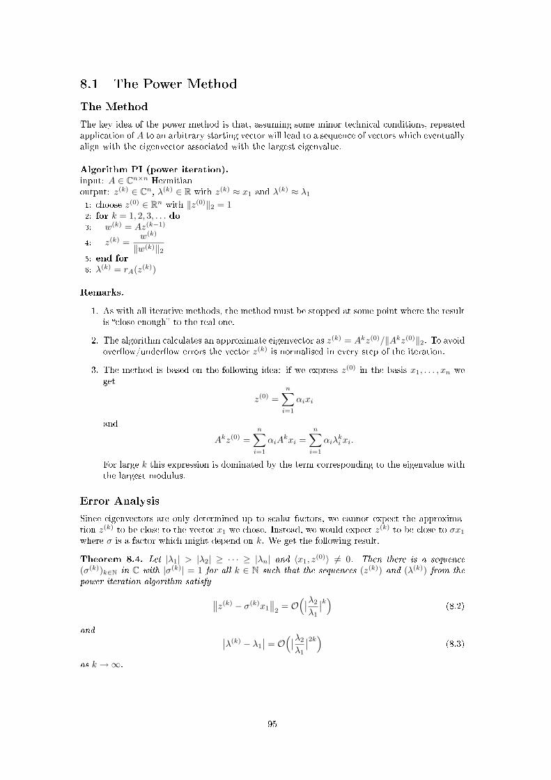
8.1 The Power Method
The Method
The key idea of the power method is that, assuming some minor technical conditions, repeatedapplication of A to an arbitrary starting vector will lead to a sequence of vectors which eventuallyalign with the eigenvector associated with the largest eigenvalue.
Algorithm PI (power iteration).input: A ∈ Cn×n Hermitianoutput: z(k) ∈ Cn, λ(k) ∈ R with z(k) ≈ x1 and λ(k) ≈ λ1
1: choose z(0) ∈ Rn with ‖z(0)‖2 = 12: for k = 1, 2, 3, . . . do3: w(k) = Az(k−1)
4: z(k) =w(k)
‖w(k)‖25: end for6: λ(k) = rA(z(k))
Remarks.
1. As with all iterative methods, the method must be stopped at some point where the resultis close enough to the real one.
2. The algorithm calculates an approximate eigenvector as z(k) = Akz(0)/‖Akz(0)‖2. To avoidoverow/underow errors the vector z(k) is normalised in every step of the iteration.
3. The method is based on the following idea: if we express z(0) in the basis x1, . . . , xn weget
z(0) =n∑i=1
αixi
and
Akz(0) =n∑i=1
αiAkxi =
n∑i=1
αiλki xi.
For large k this expression is dominated by the term corresponding to the eigenvalue withthe largest modulus.
Error Analysis
Since eigenvectors are only determined up to scalar factors, we cannot expect the approxima-tion z(k) to be close to the vector x1 we chose. Instead, we would expect z(k) to be close to σx1
where σ is a factor which might depend on k. We get the following result.
Theorem 8.4. Let |λ1| > |λ2| ≥ · · · ≥ |λn| and 〈x1, z(0)〉 6= 0. Then there is a sequence
(σ(k))k∈N in C with |σ(k)| = 1 for all k ∈ N such that the sequences (z(k)) and (λ(k)) from thepower iteration algorithm satisfy ∥∥z(k) − σ(k)x1
∥∥2
= O(∣∣λ2
λ1
∣∣k) (8.2)
and ∣∣λ(k) − λ1
∣∣ = O(∣∣λ2
λ1
∣∣2k) (8.3)
as k →∞.
95
Proof. a) We can write z(0) as
z(0) =n∑i=1
αixi, αi = 〈xi, z(0)〉.
Since α1 = 〈x1, z(0)〉 6= 0, we get
Akz(0) =n∑i=1
αiλki xi = α1λ
k1
(x1 +
n∑i=2
αiα1
( λiλ1
)kxi
)and Pythagoras' Theorem gives∥∥Akz(0)
∥∥ 2
2= |α1λ
k1 |2(
1 +n∑i=2
∣∣αiα1
∣∣2∣∣ λiλ1
∣∣2k) = |α1λk1 |2(1 + γk)
where
γk =n∑i=2
∣∣αiα1
∣∣2∣∣ λiλ1
∣∣2k ≤ ‖z(0)‖22|α1|2
∣∣λ2
λ1
∣∣2k.Thus we can conclude
z(k) =Akz(0)
‖Akz(0)‖2=
α1λk1
|α1λk1 |
(x1 +
n∑i=2
αiα1
( λiλ1
)kxi
) 1√1 + γk
.
Now dene σ(k) = α1λk1/|α1λ
k1 |. Then∥∥∥Akz(0)
|α1λk1 |− σ(k)x1
∥∥∥ 2
2=∥∥∥Akz(0)
α1λk1− x1
∥∥∥ 2
2=
n∑i=2
(αiα1
)2( λiλ1
)2k = γk
and thus ∥∥∥z(k) − σ(k)x1
∥∥∥2≤∥∥∥ Akz(0)
‖Akz(0)‖2− Akz(0)
|α1λk1 |
∥∥∥2
+∥∥∥Akz(0)
|α1λk1 |− σ(k)x1
∥∥∥2
=√
1 + γk − 1 +√γk
≤ 2√γk
≤ 2‖z(0)‖2|α1|
∣∣λ2
λ1
∣∣k.This completes the proof of (8.2).
b) Using part b) of Theorem 8.3 and (8.2) we get∣∣λ(k) − λ1
∣∣ =∣∣rA(z(k))− rA(σ(k)x1)
∣∣ = O(‖z(k) − σ(k)x1‖ 2
2
)= O
(∣∣λ2
λ1
∣∣2k).This completes the proof of (8.3).
Computational Complexity
For simplicity assume that our primary interest is in the accuracy of eigenvectors. We wish toiterate until
‖z(k) − σ(k)x1‖2 ≤ ε. (8.4)
Inspection of the preceding proof shows that this inequality will be attained provided
2(‖z(0)‖2
α1
)∣∣λ2
λ1
∣∣k ≤ ε. (8.5)
Hence it suces to choose k to be the smallest integer greater than
k# =ln ε−1 + ln ‖z(0)‖2 + ln 2− lnα1
ln(λ1/λ2).
96
Assumption 8.5. The rst and second eigenvalues of A satisfy λ1λ2
= 1 + Θ(n−β).
Theorem 8.6. Under Assumption 8.5 and the assumptions of Theorem 8.4, the computational
cost of using the power method to achieve (8.4) is bounded above by c(n1+β ln ε−1 + n3
), for
some constant c independent of n and ε.
Proof. Because of ‖z(0)‖2 = 1, the quantities ‖z(0)‖ and α1 are independent of n. The costof reducing A to Hessenberg (tridiagonal) form is Θ(n3) (see Lemma 4.12). Each step of theiteration then costs Θ(n), since matrix vector-multiplication and inner-products are both Θ(n)when the matrix tridiagonal. Combining the second and third items gives a bound of Θ(nβ ln ε−1)for the number of iterations. Using (8.5) gives the desired result for the largest eigenvalue andcorresponding eigenvector of the tridiagonal matrix. Transforming back to the original matrixA costs Θ(n2) and is hence negligible relative to the cost of transforming to Hessenberg form.The transformation is an orthogonal one and hence does not change the 2-norm of the error inthe eigenvector.
8.2 Inverse Iteration
The Method
The power iteration algorithm helps to nd the eigenvalue with the largest modulus and the cor-responding eigenvector. The following simple idea leads to a modication of the power iterationmethod to nd dierent eigenvalues of A.
Given λ ∈ R, the matrix (A − λI)−1 has eigenvalues µi = 1/(λi − λ) for i = 1, . . . , n.The power iteration method applied to this matrix will thus return an approximation for theeigenvector corresponding to the µj with the biggest modulus. This is the µj where λj is theeigenvalue closest to λ. The resulting algorithm is called the inverse iteration method.
Algorithm II (inverse iteration).input: A ∈ Cn×n Hermitian, λ ∈ Routput: z(k) ∈ Cn, λ(k) ∈ R with z(k) ≈ xj and λ(k) ≈ λj
where λj is the eigenvalue closest to λ
1: choose z(0) ∈ Rn with ‖z(0)‖2 = 12: for k = 1, 2, 3, . . . do3: solve (A− λI)w(k) = z(k−1)
4: z(k) =w(k)
‖w(k)‖25: end for6: return λ(k) = rA(z(k)).
Remark. For practical usage the method is stopped at some point where the result is closeenough to the real one.
Error Analysis
The following convergence result is a direct consequence of Theorem 8.4.
Theorem 8.7 (Convergence of Inverse Iteration). Let A ∈ Cn×n be Hermitian and λ ∈ R.Suppose a, b ∈ 1, . . . , n are such that |λa−λ| < |λb−λ| ≤ |λj−λ| for all j ∈ 1, . . . , n\a, b.Then, if 〈z(0), xa〉 6= 0, there exists a sequence (σ(k))k∈N with |σ(k)| = 1 such that
‖z(k) − σ(k)xa‖22 + |λ(k) − λa| = O
(∣∣∣∣λ− λaλ− λb
∣∣∣∣2k).
97
Computational Complexity
The computational cost is analogous to that of the power iteration, under appropriate assump-tions, found by translating the theorem for the power method, where we iterate A, to the inverseiteration situation where we iterate (A − λI)−1. Because, after preprocessing, A is tridiagonalthe cost of each step of inverse iteration is the same as for the power method.
8.3 Rayleigh Quotient Iteration
The Method
For inverse iteration it is necessary to estimate the eigenvalue in advance. An alternative is toestimate the eigenvalue during the course of the algorithm:
Algorithm RQI (Rayleigh quotient iteration).input: A ∈ Cn×n symmetricoutput: z(k) ∈ Rn, λ(k) ∈ R with z(k) ≈ xj and λ(k) ≈ λj for some j ∈ 1, · · · , n1: choose z(0) such that ‖z(0)‖2 = 1, λ(0) ∈ R2: for k = 1, 2, . . . do3: [A− λ(k−1)I]w(k) = z(k−1)
4: z(k) = w(k)/‖w(k)‖2
5: λ(k) =〈z(k−1), w(k)〉+ λ(k−1)‖w(k)‖22
‖w(k)‖226: end for
Notice that λ(k) in step 5 is simply rA(w(k)), computed without application of A.
Error Analysis
The previous two algorithms both converged linearly: asymptotically, the error decreases by aconstant factor at each step. In contrast, when the Rayleigh quotient iteration converges to aneigenvalue, say λj , it does so cubically:
|λ(k+1) − λj | = O(|λ(k) − λj |3).
A similar cubic rate of convergence is also obtained for the eigenvector. Such methods can hencebe very ecient.
Computational Complexity
However, with iterations of this type, where the convergence is not linear (as with the New-ton method for example), it is dicult to predict when it will converge, and to which eigen-value/eigenvector pair it will converge. Much of the computational complexity of such algorithmsstems from choosing starting points which will lead to convergence to the desired pair.
8.4 Simultaneous Iteration
The Method
Now imagine that we wish to calculate all the eigenvectors. A natural idea is to take
z(0) ∈ Rn×n
orthonormal, and generateZ(k+1) = AZ(k).
98
Then each column of Z(k), z(k)i , is calculated as
z(k+1)i = Az
(k)i .
Let
z(0)i =
n∑j=1
αj,ixj
and assume thatαi,i = 〈z(0)
i , xi〉 6= 0, i = 1, . . . , n (8.6)
Now
z(k)i =
n∑j=1
αj,iλkjxj .
If|λ1| > |λ2| > · · · > |λn−1| > |λn| (8.7)
then
spanz(k)1 = spany1, ‖y1‖2 = 1, y1 = x1 + e1
spanz(k)1 , z
(k)2 = spany1, y2, ‖y2‖2 = 1, y2 = x2 + e2
...
spanz(k)1 , z
(k)2 , . . . , z(k)
n = spany1, y2, . . . , yn, ‖yn‖2 = 1, yn = xn + en,
where
ej =minj,n−1∑
l=1
O
(∣∣∣∣λl+1
λl
∣∣∣∣k)
= O(ξ)
for
ξ := max1≤l≤n−1
λl+1
λl.
However, in practice this is a poor algorithm, not only because of overow / underow if
|λ1| 6= 1, but also because the approximate basis z(k)1 , z
(k)2 , . . . , z
(k)n for x1, . . . , xn is highly
ill-conditioned, here meaning that the vectors nearly all point in the same direction, x1.To overcome these problems the algorithm used in practice forms an orthonormal basis from
the approximate basis for x1, . . . , xn, by means of QR.
Algorithm (simultaneous iteration).input: A ∈ Rn×n symmetric
output: Z(k),Λ(k) ∈ Rn×n with Z(k) ≈ (x1, x2, . . . , xn) and Λ(k)ii ≈ λi for i = 1, . . . , n
1: choose an orthogonal matrix Z(0) ∈ Rn×n2: for k = 1, 2, 3, . . . do3: W (k) = AZ(k−1)
4: calculate the QR factorisation W (k) = Z(k)R(k)
5: Λ(k) = (Z(k−1))TW (k)
6: end for
Here Z(k)R(k) is the QR factorisation of W (k). In the following we write Z(k) and W (k) interms of columns:
Z(k) = (z(k)1 , . . . , z(k)
n ), W (k) = (w(k)1 , . . . , w(k)
n ).
We show below that the diagonal entries of Λ(k) are rA(z(k−1)i ).
99
Error Analysis
Theorem 8.8 (Convergence of Simultaneous Iteration). Let A ∈ Rn×n be symmetric, satisfying
(8.7) so that ξ < 1. Under assumption (8.6) there are, for j = 1, . . . , n, sequences s(k)j k∈Z+ ,
s(k)j ∈ −1,+1, such that
‖z(k)j − s(k)
j xj‖22 + |Λ(k)jj − λj | = O(|ξ|2k).
Proof. By the discussion preceding the algorithm the result follows for the approximate eigen-vectors. Since
Λ(k)jj = 〈z(k−1)
j , w(k)j 〉 = 〈z(k−1)
j , Az(k−1)j 〉
= rA(z(k−1)j ),
the convergence to the eigenvalues follows by Theorem 8.3.
Computational Complexity
In practice the simultaneous iteration is usually implemented in the form known as the QRalgorithm, which we discuss in the next section. Hence we discuss complexity in that context.
8.5 The QR Algorithm for Eigenvalues
The Method
In practice the eigenvalues of A can be found directly by a method related to simultaneousiteration, and which we now derive. The resulting algorithm appears almost magical upon rstsight, but when related to simultaneous iteration, its mechanism is clear. To establish thisrelation let Z(k−1), Z(k), R(k), W (k) and Λ(k) be as in the simultaneous iteration algorithm anddene
Q(k) := (Z(k−1))TZ(k).
This is an orthogonal matrix by construction.Recall that
Λ(k) = (Z(k−1))TAZ(k−1).
Thus
Q(k)R(k) = (Z(k−1))TZ(k)(Z(k))TW (k)
= (Z(k−1))TAZ(k−1)
= Λ(k).
Furthermore
R(k)Q(k) = (Z(k))TW (k)(Z(k−1))TZ(k)
= (Z(k))TAZ(k)
= Λ(k+1).
Thus reversing the order of Q and R results in an improved estimate of the eigenvalues. Thissuggests the following algorithm for locating eigenvalues of A.
QR for eigenvalues input: A ∈ Rn×n symmetricoutput: Λ ∈ Rn×n with diagonal entries approximating the eigenvalues
1: Set Λ(0) = A2: for k = 1, 2, . . . do3: calculate the QR factorisation Λ(k−1) = Q(k−1)R(k−1)
4: Λ(k) = R(k−1)Q(k−1)
5: end for
100
Error Analysis
Theorem 8.9 (Convergence of QR). Under the assumptions of Theorem 8.8, the QR eigenvaluealgorithm satises (possibly after reordering of eigenvalues)
‖Λ(k)ii − λi‖2 = O
(|ξ|2k
), ∀i = 1, · · · , n.
Proof. The algorithm produces the same Λ(k) as simultaneous iteration. So the diagonal be-haviour follows from Theorem 8.8.
For the o-diagonals, note that by orthogonality of the xl
Λ(k)jl = 〈z(k)
j , Az(k)l 〉 = 〈xj , Axl〉+O(|ξ|k)
= 〈xj , λlxl〉+O(|ξ|k)
= λl〈xj , xl〉+O(|ξ|k)
= O(|ξ|k).
Thus the matrix Λ becomes diagonal as k →∞.
Computational Complexity
Making the error in the QR method of size ε gives the number of iterations k = O(ln εln ξ
). Under
the assumptions of Theorem 8.8, the QR algorithm as stated would cost
O(
ln εln ξ
n3
)work to obtain estimates of all eigenvalues to within O(ε). However, this can be improved to
O(
ln εln ξ
n2
)+O(n3),
with second term independent of ε, ξ as follows.Recall from Denition 1.8 that a matrix A ∈ Cn×n is upper Hessenberg if
aij = 0 i > j + 1.
Lemma 8.10. If Λ(0) is upper Hessenberg, the QR Algorithm generates Λ(k) which are upperHessenberg.
Proof. We have
Λ(k) = R(k−1)Q(k−1)
= R(k−1)Λ(k−1)(R(k−1))−1.
But R(k−1) and its inverse are upper triangular and pre- or post-multiplication by upper trian-gular matrices preserves the upper Hessenberg form.
Theorem 8.11 (Cost of QR). Under the assumptions of Theorem 8.8 the QR algorithm can beimplemented to give eigenvalue approximations of size ε with cost
C(n, ε) ≤ k1ln εln ξ
n2 + k2n3,
where k1, k2 are independent of n, ε and ξ.
Proof. (Sketch) First nd T as in Lemma 4.12, at cost Θ(n3). Then apply the QR algorithm toT . Since each QR factorisation is on an upper Hessenberg matrix, the cost reduces to Θ(n2).The number of iterations required to reduce the error to size ε is bounded by O(ln ε/ ln ξ) andthe result follows.
101
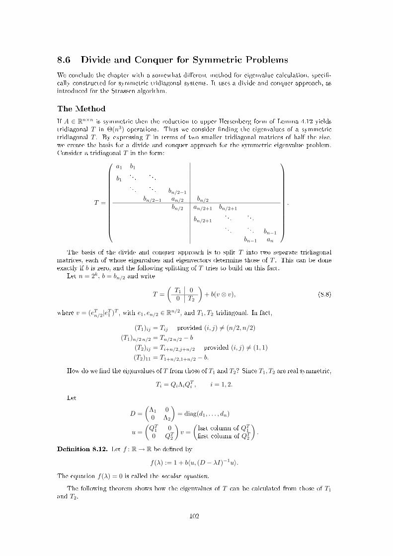
8.6 Divide and Conquer for Symmetric Problems
We conclude the chapter with a somewhat dierent method for eigenvalue calculation, speci-cally constructed for symmetric tridiagonal systems. It uses a divide and conquer approach, asintroduced for the Strassen algorithm.
The Method
If A ∈ Rn×n is symmetric then the reduction to upper Hessenberg form of Lemma 4.12 yieldstridiagonal T in Θ(n3) operations. Thus we consider nding the eigenvalues of a symmetrictridiagonal T . By expressing T in terms of two smaller tridiagonal matrices of half the size,we create the basis for a divide and conquer approach for the symmetric eigenvalue problem.Consider a tridiagonal T in the form:
T =
a1 b1
b1. . .
. . .
. . .. . . bn/2−1
bn/2−1 an/2 bn/2bn/2 an/2+1 bn/2+1
bn/2+1
. . .. . .
. . .. . . bn−1
bn−1 an
.
The basis of the divide and conquer approach is to split T into two separate tridiagonalmatrices, each of whose eigenvalues and eigenvectors determine those of T . This can be doneexactly if b is zero, and the following splitting of T tries to build on this fact.
Let n = 2k, b = bn/2 and write
T =(T1 00 T2
)+ b(v ⊗ v), (8.8)
where v = (eTn/2|eT1 )T , with e1, en/2 ∈ Rn/2, and T1, T2 tridiagonal. In fact,
(T1)ij = Tij provided (i, j) 6= (n/2, n/2)(T1)n/2n/2 = Tn/2n/2 − b
(T2)ij = Ti+n/2,j+n/2 provided (i, j) 6= (1, 1)(T2)11 = T1+n/2,1+n/2 − b.
How do we nd the eigenvalues of T from those of T1 and T2? Since T1, T2 are real symmetric,
Ti = QiΛiQTi , i = 1, 2.
Let
D =(
Λ1 00 Λ2
)= diag(d1, . . . , dn)
u =(QT1 00 QT2
)v =
(last column of QT1rst column of QT2
).
Denition 8.12. Let f : R→ R be dened by
f(λ) := 1 + b〈u, (D − λI)−1u〉.
The equation f(λ) = 0 is called the secular equation.
The following theorem shows how the eigenvalues of T can be calculated from those of T1
and T2.
102
Theorem 8.13. Assume that the di are distinct and that ui 6= 0 for all i. Then the eigenvaluesof T are the real roots of the secular equation.
Proof.
T =(Q1Λ1Q
T1 0
0 Q2Λ2QT2
)+ bv ⊗ v
=(Q1 00 Q2
)((Λ1 00 Λ2
)+ bu⊗ u
)(QT1 00 QT2
).
Thus T has the same eigenvalues as D + bu⊗ u by similarity.Now,
det(D + bu⊗ u− λI) = det((D − λI)(I + b(D − λI)−1u⊗ u)).
Ifdet(D + bu⊗ u− λI) = 0
and λ is not an eigenvalue of D then
det(I + b(D − λI)−1u⊗ u) = 0.
Now det(I + x⊗ y) = 1 + 〈y, x〉 (see Exercise 8-4) and so
1 + b〈u, (D − λI)−1u〉 = f(λ) = 0.
Recall that we assume the di are distinct and that ui 6= 0. Let d0 = −∞ and dn+1 = ∞.Then
• if b < 0 then f(λ) has n roots λi ∈ (di, di+1), i = 0, . . . , n− 1;
• if b > 0 then f(λ) has n roots λi ∈ (di, di+1), i = 1, . . . , n.
This follows from the fact that
f(λ) = 1 + b
n∑i=1
u2i
(di − λ).
Hence all the eigenvalues are accounted for and it follows that the assumption that λ cannot bean eigenvalue of D holds.
Theorem 8.13 is the basis of a divide and conquer algorithm for the eigenvalue problem.
Error Analysis
The primary source of error, in real arithmetic, arises from solution of the secular equation.However, because the roots which we seek are real, and because they lie in known intervals,root-nding methods with great accuracy and eciency can be applied (a simple example beingbisection). In practice the errors arising from this step of the algorithm are negligible comparedwith those arising from nite precision arithmetic.
Computational Complexity
Let Lk = C(2k), where C(n) is the cost of nding eigenvalues and eigenvectors of symmetrictridiagonal matrices in Rn×n. If we use a recursive algorithm, then the cost Lk needs to beexpressed in terms of the cost Lk−1 of nding the eigenvalues and eigenvectors of symmetrictridiagonal matrices in Rn/2×n/2.
Finding the eigenvalues and eigenvectors in Rn×n has cost Lk where
Lk = 2Lk−1 +mk,
where mk is the cost of constructing, and solving, the secular equation for T ∈ Rn×n. This costcomprises:
103
• nding eigenvectors from these eigenvalues: this costs Θ(n) for each eigenvalue since thematrix is tridiagonal, giving a total of Θ(n2);
• constructing u: Θ(n) to nd last column of QT1 and rst column of QT2 ;
• Solving the secular equation: Θ(n), assuming unit cost for each root using, for example,bisection.
To state a theorem about the cost of this iteration we need the following denition.
Denition 8.14. The decomposition (8.8) of a tridiagonal matrix T is non-degenerate if thedi are distinct and ui 6= 0 for all i.
Theorem 8.15 (Cost of Eigenvalue Divide and Conquer). Let T be symmetric, tridiagonal. Ifall decompositions are non-degenerate at each level of recursion and if root nding for the secularequation is assigned unit cost, then the algorithm generates all eigenvalues and eigenvectors ofT at cost O(n2).
Proof. We have mk = Θ(n2) = Θ(4k). Thus, for some a > 0,
Lk ≤ 2Lk−1 + a4k.
Induction based on the assumptionLk ≤ b4k
gives the desired result, provided b ≥ min1, 2a, since nding the eigenvalues of a 1× 1 matrixhas unit cost.
Bibliography
The book [Par80] contains a very complete overview of the symmetric eigenvalue problem, thesubject that dominates this chapter. The book [TB97] has a good introduction to the subject.
Exercises
Exercise 8-1. The purpose of this question is to introduce you to ideas associated with eigen-value problems and their solution in Matlab. The basic problem is, given A ∈ Rn×n, to ndx ∈ Cn and λ ∈ C such that
Ax = λx (8.9)
and, of course, x should be non-zero.(i) What can you say about the eigenvalues λ if A is symmetric (just state, no proof). Whatcan you say about the eigenvectors?(ii) Write down the denition of the characteristic polynomial satised by the eigenvalues λ.(iii) What is the polynomial in the case >> A=[3,2; 1,2] Hence nd the eigenvalues and eigen-vectors.(iv) If
>> A=[3,2,1; 2,2,2; 1,2,1]
write the polynomial for λ in the form
p1λ3 + p2λ
2 + p3λ+ p4 = 0
and nd p = (p1, p2, p3, p4). In principle you can solve this cubic exactly so there is no need toresort to numerical solution. (In general we obtain
n∑i=0
λn−ipi+1 = 0.
What does Galois tell us about our need for applying numerical solutions to this problem?)(v) One way to nd the eigenvalues of A is to use the Matlab command roots. Type
104
>> roots(p)
to nd the roots of our cubic, and hence the eigenvalues of A. We can do this more generally.Type
>> A=randn(20);
>> A=0.5*[A+A'];
>> p=poly(A)'
This creates a 20 × 20 matrix with normally distributed random entries, and then makes asymmetric matrix from A. The vector p contains the co-ecients in the characteristic polynomialof A so that, if you type sort(roots(p)) you will get the eigenvalues of A (sort just orders theroots). Do this.(vi) Thus one way to nd eigenvalues of A in Matlab is to form the characteristic polynomialand nds its roots. But Matlab does not do this as more ecient methods are available. Type
>> sort(eig(A))
and you should get the same as you did in (v). But the method employed was very dierent.Here we show you the two key ideas used in eig. Set
>> A=[-1,2,3,0,4;2,1,6,2,2;3,6,3,3,0;0,2,3,8,2;4,2,0,2,-1]
and now type
>> [Q,H]=hess(A)
What properties do Q and H have? Type
>> rn=norm(Q*H*Q'-A)
What can you say about the relationship between the eigenvalues of H and those of A?Now type
>> [W,D]=schur(H)
What properties do W and D have? Type
>> rn=norm(W*D*W'-H)
What can you say about the relationship between the eigenvalues of D and those of H?Finally, what can you say about the relationship between the eigenvalues of A and the
diagonal elements of D? Test your hypothesis by typing eig(A) and comparing with D.
Exercise 8-2. Give a proof by induction which shows that the matrix A from (8.1) really hasdeterminant (−1)np(z) where p(z) = a0 + a1z + · · ·+ an−1z
n−1 + zn.
Exercise 8-3. Let B be a constant matrix and let T (t) solve the matrix dierential equation
dT
dt= BT − TB, T (0) = T0.
Assuming that the solution of this equation exists for all t ∈ R, show that T (t) has the sameeigenvalues as T0, for all t ∈ R. If B is skew-symmetric, show that ‖T (t)‖2 = ‖T0‖2 for all t ∈ R.
Exercise 8-4. Prove that det(I + xyT ) = 1 + yTx.
Exercise 8-5. Construct an example showing that the Jordan canonical form of a matrix canbe discontinuous with respect to small perturbations.
105
Exercise 8-6. Newton's Method
1. Let G : Rm → Rm be dierentiable. Newton's method for the solution of the equationG(y) = 0 is to generate iterates yk according to
dG(yk)δyk = −G(yk), yk+1 = yk + δyk
where dG(y) is the Jacobian of G evaluated at y. Find the explicit formula for yk+1 interms of yk when m = 1. What is the order of convergence of the method?
2. The eigenvalue problem for A ∈ R can be regarded as a nonlinear system of equations fory = y(x, λ) satisfying
Ax− λx = 012
(xTx− 1) = 0
Apply Newton's method to this system and show that it gives the iteration
λk+1 = λk +12 (‖xk‖22 + 1)
xTk (A− λkI)−1xk
xk+1 = (λk+1 − λk)(A− λkI)−1xk.
If x0 = α0ϕ (α20 6= 1), Aϕ = µϕ (‖ϕ‖2 = 1) and λ0 6= µ, show that xk = αkϕ and nd the
iteration governing the αk, i.e. nd h : R→ R such that
αk+1 = h(αk).
Show that this iteration is Newton's method applied to a scalar equation and identify thatequation. Using this fact, prove that the full method on Rm is second order convergent forthis specic choice of initial data.
Exercise 8-7. Prove the following theorem concerning eigenvalues of tridiagonal matrices.
Theorem 8.16. Consider a matrix A of the form (5.5). Let the diagonal entries be real, constantwith equal o-diagonal entries: ai = a, ci = a and di = d for all i = 1, . . . ,m where a and d arereal. Then the eigenvalues λk of the matrix are given by
λk = d+ 2a cos(
kπ
m+ 1
),
for k = 1, . . . ,m. The corresponding eigenvector x = [x1, . . . , xm]T has jth component given by
xj = sin(kπj/(m+ 1)) (8.10)
Exercise 8-8. Consider the companion matrix C from (8.1). Prove that the eigenvalues λkof C are the roots of the polynomial
m∑j=0
αjλj = 0
where αm = 1. The corresponding eigenvector is
x = [x1, . . . , xm]T
where xj = λj−1k .
106
Bibliography
[Bha97] R. Bhatia. Matrix Analysis. Springer, 1997.
[CH96] S.-N. Chow and J.K. Hale. Methods of Bifurcation Theory. Springer, 1996.
[CLRS01] T.H. Cormen, C.E. Leiserson, R.L. Rivest, and C. Stein. Introduction to Algorithms.McGraw Hill, 2001.
[Dem97] J.W. Demmel. Applied Numerical Linear Algebra. SIAM, 1997.
[GL96] G. Golub and C. Van Loan. Matrix Computations. Johns Hopkins, third edition,1996.
[Hig02] N.J. Higham. Accuracy and Stability of Numerical Algorithms. SIAM, 2002.
[HJ85] R.A. Horn and JC.R. Johnson. Matrix Analysis. Cambridge University Press, 1985.
[Lax97] P. Lax. Linear Algebra. Wiley, 1997.
[LT88] Randall J. Leveque and Lloyd N. Trefethen. Fourier analysis of the SOR iteration.IMA Journal of Numerical Analysis, 8(3):273279, 1988.
[Ner71] E.D. Nering. Linear Algebra and Matrix Theory. John Wiley, 1971.
[NW06] J. Nocedal and S.J. Wright. Numerical Optimization. Springer, 2006.
[Par80] B. Parlett. The Symmetric Eigenvalue Problem. Prentice-Hall, 1980.
[Rob01] J.C. Robinson. Innite Dimensional Dynamical Systems. CUP, 2001.
[Saa97] Y. Saad. Iterative Methods for Sparse Linear Systems. PWS, 1997.
[SB02] J. Stoer and R. Bulirsch. Introduction to Numerical Analysis. Springer, third edition,2002.
[TB97] L.N. Trefethen and D. Bau. Numerical Linear Algebra. SIAM, 1997.
107