Matlab Lab 1 Solutions  

Problem 1 

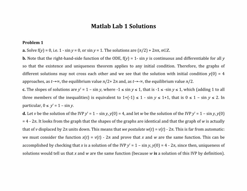
a. Solve f(y) = 0, i.e. 1 ‐ sin y = 0, or sin y = 1. The solutions are (π/2) + 2nπ, n∈Ζ. 

b. Note that the right‐hand‐side function of the ODE, f(y) = 1‐ sin y is continuous and differentiable for all y 

so  that  the  existence  and  uniqueness  theorem  applies  to  any  initial  condition.  Therefore,  the  graphs  of 

different  solutions may  not  cross  each  other  and we  see  that  the  solution with  initial  condition  y(0)  =  4 

approaches, as t→∞, the equilibrium value π/2+ 2π and, as t→‐∞, the equilibrium value π/2. 

c. The slopes of solutions are y’ = 1 – sin y, where ‐1 ≤ sin y ≤ 1, that is ‐1 ≤ ‐sin y ≤ 1, which (adding 1 to all 

three members  of  the  inequalities)  is  equivalent  to  1+(‐1) ≤  1  ‐  sin  y ≤  1+1,  that  is  0 ≤  1  –  sin  y ≤  2.  In 

particular, 0 ≤  y’ = 1 – sin y. 

d. Let v be the solution of the IVP y’ = 1 – sin y, y(0) = 4, and let w be the solution of the IVP y’ = 1 – sin y, y(0) 

= 4 ‐ 2π. It looks from the graph that the shapes of the graphs are identical and that the graph of w is actually 

that of v displaced by 2π units down. This means that we postulate w(t) = v(t) ‐ 2π. This is far from automatic: 

we must  consider  the  function x(t) = v(t)  ‐ 2π  and prove  that x  and w  are  the  same  function. This  can be 

accomplished by checking that x is a solution of the IVP y’ = 1 – sin y, y(0) = 4 ‐ 2π, since then, uniqueness of 

solutions would tell us that x and w are the same function (because w is a solution of this IVP by definition). 

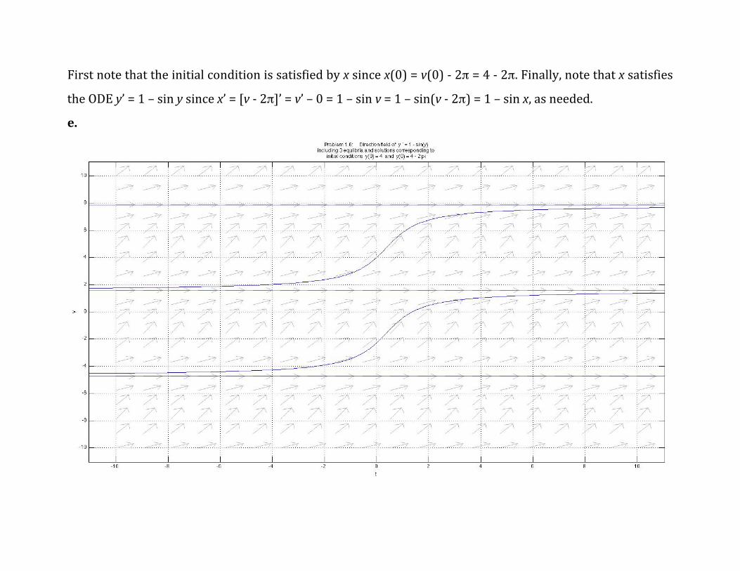
First note that the initial condition is satisfied by x since x(0) = v(0) ‐ 2π = 4 ‐ 2π. Finally, note that x satisfies 

the ODE y’ = 1 – sin y since x’ = [v ‐ 2π]’ = v’ – 0 = 1 – sin v = 1 – sin(v ‐ 2π) = 1 – sin x, as needed. 

e.       

 

 

Problem 2 

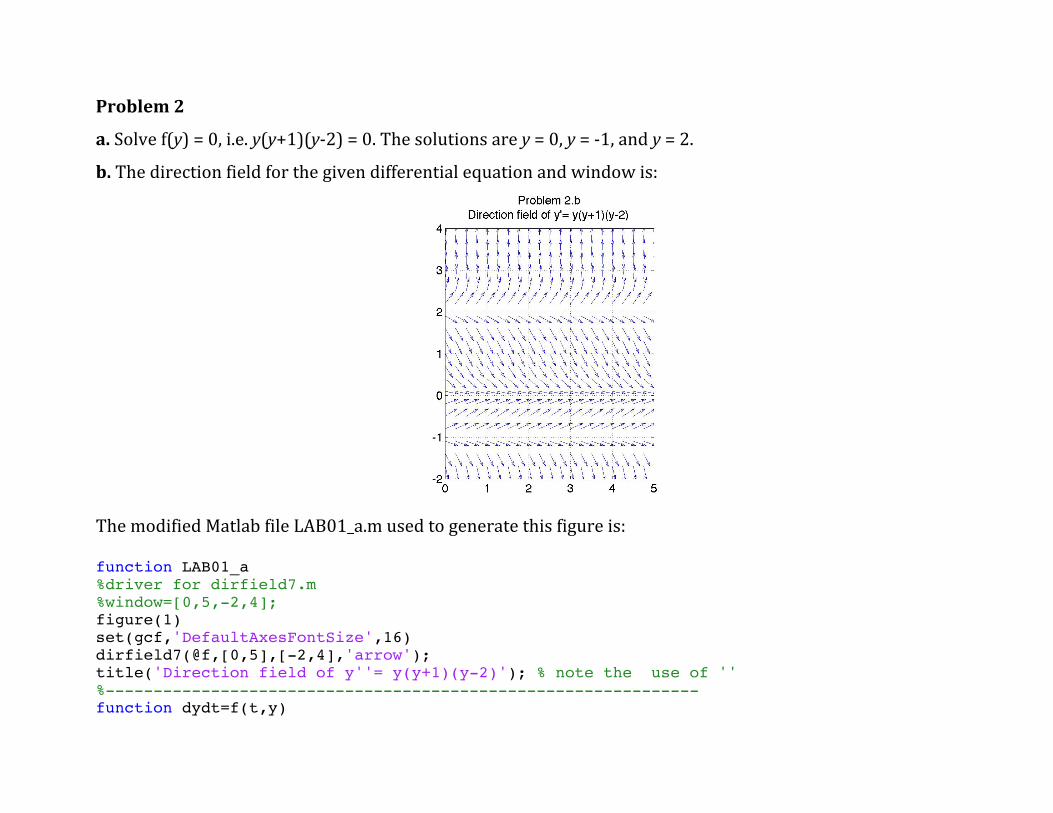
a. Solve f(y) = 0, i.e. y(y+1)(y‐2) = 0. The solutions are y = 0, y = ‐1, and y = 2. 

b. The direction field for the given differential equation and window is: 

                                                          The modified Matlab file LAB01_a.m used to generate this figure is:  function LAB01_a %driver for dirfield7.m %window=[0,5,-2,4]; figure(1) set(gcf,'DefaultAxesFontSize',16) dirfield7(@f,[0,5],[-2,4],'arrow'); title('Direction field of y''= y(y+1)(y-2)'); % note the use of '' %-------------------------------------------------------------- function dydt=f(t,y)

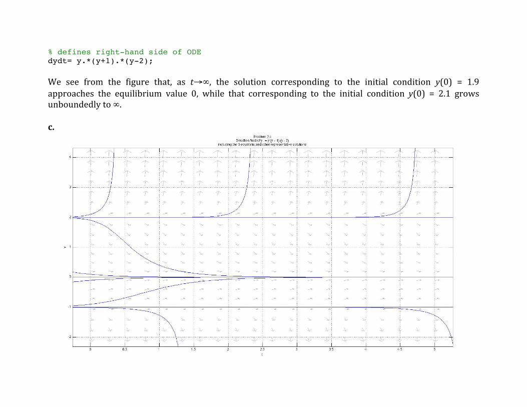
% defines right-hand side of ODE dydt= y.*(y+1).*(y-2);  We  see  from  the  figure  that,  as  t→∞,  the  solution  corresponding  to  the  initial  condition  y(0)  =  1.9 approaches  the  equilibrium  value  0,  while  that  corresponding  to  the  initial  condition  y(0)  =  2.1  grows unboundedly to ∞.  c. 

 

No two curves cross each other. The reason is that, if there was a point of intersection for 2 curves, (τ, ξ), 

say,  then  the  initial  value  problem  corresponding  to  the  initial  condition  y(τ)  =    ξ  would  have  two 

different  solutions  corresponding  to  the  2  graphs  that  pass  through  this  point.  This  contradicts  the 

uniqueness theorem, which for this ODE holds with any initial condition since the right‐hand‐side f(y) = y  

(y+1)(y‐2) is continuous and differentiable for all values of t and y. 

 

d. The solution corresponding to the initial condition y(0) = ½ cannot eventually (i.e. for any t) become ‐1 

because the constant function y = ‐1 is the solution of the ODE corresponding to the initial condition y(0) 

= ‐1 and solutions corresponding to different initial conditions at the same initial time (here t = 0) cannot 

intersect because of uniqueness. 

 

Problem 4.i 

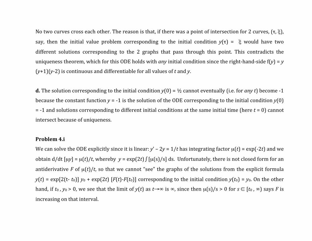
We can solve the ODE explicitly since it is linear: y’ – 2y = 1/t has integrating factor µ(t) = exp(‐2t) and we 

obtain d/dt [µy] = µ(t)/t, whereby  y = exp(2t) ∫ [µ(s)/s] ds.  Unfortunately, there is not closed form for an 

antiderivative F of µ(t)/t,  so  that we cannot “see”  the graphs of  the solutions  from the explicit  formula 

y(t) = exp[2(t‐ t0)] y0 + exp(2t) [F(t)‐F(t0)] corresponding to the initial condition y(t0) = y0. On the other 

hand, if t0 , y0 > 0, we see that the limit of y(t) as t→∞ is ∞, since then µ(s)/s > 0 for s ∈ [t0 , ∞) says F is 

increasing on that interval. 

 

a. We see in the figure that as t approaches ∞ solutions approach either ∞ or ‐∞. 

b. Yes, in some cases. It seems from the figure that the curve y = 1/(2t) separates solutions that go to ∞ 

from  those  that go  to  ‐∞  as  t  approaches ∞. Two  initial  conditions  that are arbitrarily  close, one on 

each side of the curve, lead to substantially different solutions (large changes). 

c. No periodic solutions exist here since they all approach ∞ or ‐∞. 

d. For t approaching ‐∞ all solutions seems to approach y = 0 asymptotically. 

 

Problem 4.ii 

We can solve the ODE explicitly since it is linear: y’ + ½ y = sin t has integrating factor µ(t) = exp(½ t) and we 

obtain d/dt  [µy] = µ(t)  sin  t, whereby   y(t)= C  exp(‐½t) + 2(sin  t  ‐2cos  t)/5, where C  is  an arbitrary  real 

number.  It  follows  immediately  that  for  any  initial  condition,  as  t  approaches ∞,  the  solution  of  the  IVP 

approaches the periodic function p(t) = 2(sin t  ‐2cos t)/5 = 2/√5 sin(t+α), where tan α = ‐2. This periodic 

function  can  be  expressed  in  the  standard  form  p(t)  =  A  sin(ωt+α),  where  the  amplitude  is  A  =  2/√5  ≅ 

0.8944,  the  angular  frequency  is ω  =  1,  and  the  angle  of  phase  is α ≅  ‐1.1071. Naturally,  the  behavior  of 

solutions  for  t  approaching  ‐∞  depends  on  the  sign  of  C:  they  approach ∞  if  C  is  positive  and  ‐∞  if  C  is 

negative. 

 

 

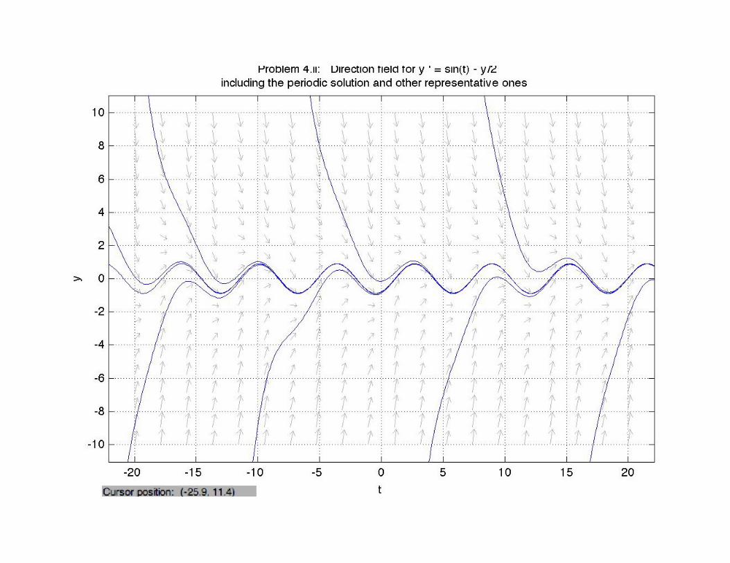
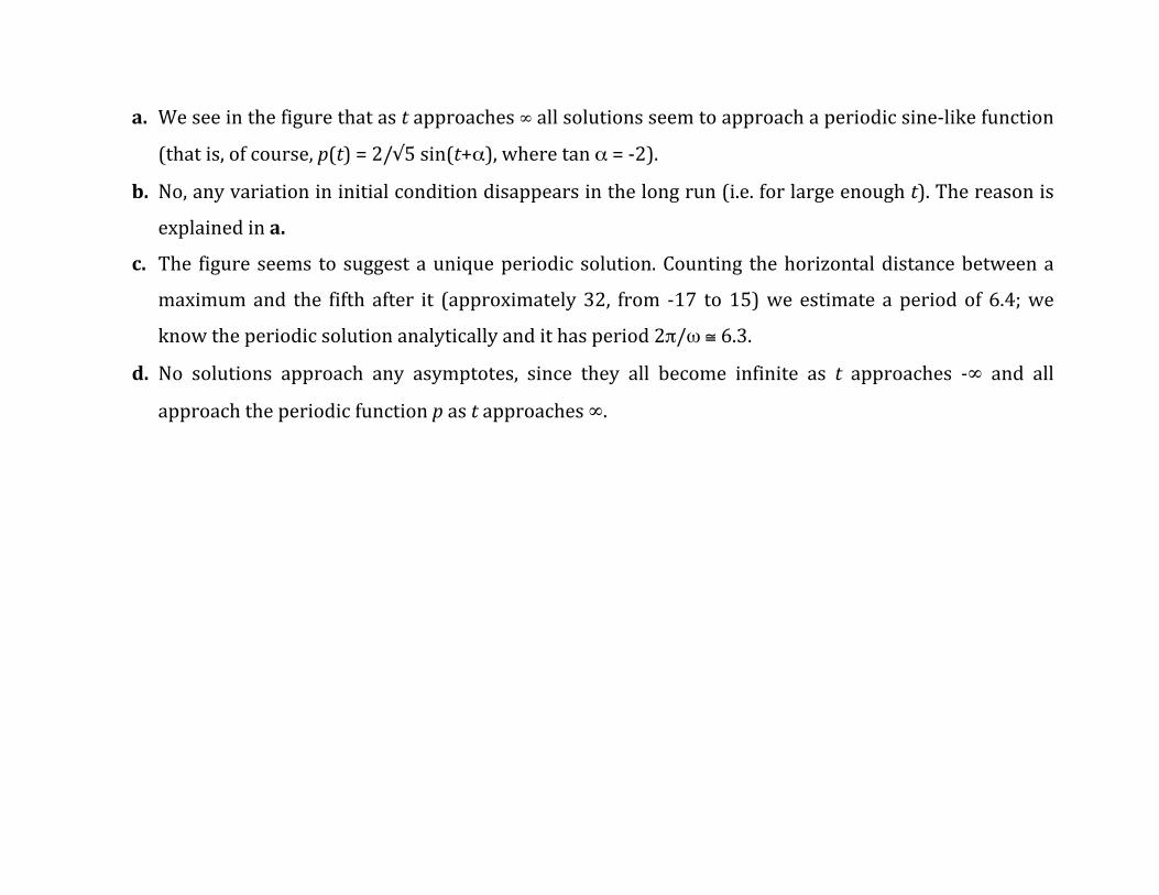
a. We see in the figure that as t approaches ∞ all solutions seem to approach a periodic sine‐like function 

(that is, of course, p(t) = 2/√5 sin(t+α), where tan α = ‐2). 

b. No, any variation in initial condition disappears in the long run (i.e. for large enough t). The reason is 

explained in a. 

c. The  figure seems  to  suggest a unique periodic  solution. Counting  the horizontal distance between a 

maximum and  the  fifth  after  it  (approximately 32,  from  ‐17  to 15) we  estimate  a period of  6.4; we 

know the periodic solution analytically and it has period 2π/ω ≅ 6.3. 

d. No  solutions  approach  any  asymptotes,  since  they  all  become  infinite  as  t  approaches  ‐∞  and  all 

approach the periodic function p as t approaches ∞.