Mathematics 611, Fall, 2010

September 30, 2010

Contents

1 Hilbert space and orthonormal bases 21.1 Norms, inner products and Schwarz inequality . . . . . . . . . 21.2 Bessel’s inequality and orthonormal bases . . . . . . . . . . . . 51.3 Problems on Hilbert space . . . . . . . . . . . . . . . . . 12

2 Generalized functions. (δ functions and all that.) 142.1 Dual spaces . . . . . . . . . . . . . . . . . . . . . . . . . . . . 142.2 Problems on Linear Functionals . . . . . . . . . . . . . . . . . 182.3 Generalized functions . . . . . . . . . . . . . . . . . . . . . . . 202.4 Derivatives of generalized functions . . . . . . . . . . . . . . . 242.5 Problems on derivatives and convergence of distribu-

tions. . . . . . . . . . . . . . . . . . . . . . . . . . . . . . . . 262.6 Distributions over Rn . . . . . . . . . . . . . . . . . . . . . . . 282.7 Poisson’s Equation . . . . . . . . . . . . . . . . . . . . . . . . 29

3 The Fourier Transform 323.1 The Fourier Inversion formula on S(R). . . . . . . . . . . . . . 363.2 Extension of the Fourier transform to L2 and other function

spaces. . . . . . . . . . . . . . . . . . . . . . . . . . . . . . . . 403.3 The Fourier transform over Rn . . . . . . . . . . . . . . . . . . 433.4 Tempered Distributions . . . . . . . . . . . . . . . . . . . . . . 463.5 Problems on the Fourier Transform . . . . . . . . . . . . 49

1

1 Hilbert space and orthonormal bases

1.1 Norms, inner products and Schwarz inequality

Definition. A norm on a real or complex vector space, V is a realvalued function, ‖ · ‖ on V such that1. a. ‖x‖ ≥ 0 for all x in V .b. ‖x‖ = 0 only if x = O.2. ‖αx‖ = |α|‖x‖ for all scalars α and all x in V .3. ‖x+ y‖ ≤ ‖x‖+ ‖y‖.Note that the converse of 1.b follows from 2. because ‖O‖ = ‖0O‖ =

0‖O‖ = 0.Examples1.1 V = R, ‖x‖ = |x|.1.2 V = C, ‖x‖ = |x|.1.3 V = Rn with ‖x‖ =

√∑n1 x

2j when x = (x1, . . . , xn).

1.4 V = Cn with ‖x‖ =√∑n

1 |xj|2 when x = (x1, . . . , xn).1.5 V = C([0, 1]). These are the continuous, complex valued functions on

[0, 1].Here are two norms on V .

‖f‖1 =

∫ 1

0

|f(t)|dt (1.1) H5.1

‖f‖∞ = sup{|f(t)| : t ∈ [0, 1]} (1.2) H5.2

Exercise 1.1 Prove that the expression in (H5.21.2) is a norm.

Here is an infinite family of other norms on Rn. Let 1 ≤ p <∞. Define

‖x‖p =( n∑j=1

|xj|p)1/p

(1.3) H5.3

FACT: These are all norms. And here is yet one more. Define

‖x‖∞ = maxj=1,...,n

|xj| (1.4) H5.4

2

Exercise 1.2 Prove that ‖x‖1 and ‖x‖∞ are norms. (Sadly, the proof that‖x‖p is a norm is not that easy. So don’t even try. We’ll prove the p = 2case later.)

The unit ball of a norm ‖ · ‖ on a vector space V is

B = {x ∈ V : ‖x‖ ≤ 1} (1.5)

A picture of the unit ball of a norm gives some geometric insight into thenature of the norm. Its especially illuminating to compare norms by compar-ing their unit balls. Lets consider the family of norms defined in (

H5.31.3) and

(H5.41.4) on R2. The boundary of each unit ball is the curve ‖x‖ = 1 and clearly

goes through the points (1, 0) and (0, 1). Its not hard to compute that theunit ball of ‖ · ‖∞ is a square with sides parallel to the coordinate axes. Theunit ball of ‖ · ‖2 is a disk contained in this square, and unit ball of ‖ · ‖1 isa diamond shape thing contained in this disk. Less obvious, but reasonable,is the fact that the other unit balls lie inside the square and contain thediamond. Draw pictures.

Definition An inner product on a real or complex vector space Vis a function on V × V to the scalars such that1. (x, x) ≥ 0 for all x ∈ V and (x, x) = 0 only if x = 0.2. (ax+ by, z) = a(x, z) + b(y, z) for all scalars a, b and all vectors x, y.3. (x, y) = (y, x).Examples1.6 V = Rn with (x, y) =

∑nj=1 xjyj.

1.7 V = Cn with (x, y) =∑n

1 xjyj1.8 V = C([0, 1]) with (f, g) =

∫ 1

0f(t)g(t)dt. [It would be good for you

to verify yourself that this really is an inner product.]1.9 V = l2, which is the standard notation for the set of sequences x =

(a1, a2, . . . ) such that∑∞

k=1 |ak|2 <∞. Define

(x, y) =∞∑k=1

akbk

when y = (b1, b2, . . . ). The series entering into this definition convergesabsolutely because of the identity |ab| ≤ (|a|2 + |b|2)/2. [It would be verygood for you to verify that this really defines an inner product on l2.]

3

Theorem 1.1 ( The Schwarz inequality.) In any inner product space

|(x, y)| ≤ (x, x)1/2(y, y)1/2 (1.6) H2

Proof: If x or y is zero then both sides are 0. So we can assume x 6= 0and y 6= 0. In case the inner product space is complex choose α ∈ C suchthat |α| = 1 and α(x, y) is real. If the inner product space is real just takeα = 1. In either case let p(t) = ‖αx+ ty‖2 for all t ∈ R. Then

0 ≤ p(t) = (αx+ ty, αx+ ty) = ‖x‖2 + t2‖y‖2 + 2t(αx, y)

because (αx, y) + (y, αx) = 2Re(αx, y) = 2(αx, y). So, by the quadraticformula, the discriminant, b2− 4ac ≤ 0. That is , 4(αx, y)2− 4‖x‖2‖y‖2 ≤ 0.Thus|α(x, y)|2 ≤ ‖x‖2‖y‖2. Now use |α| = 1. QED.

We are going to show next that in an inner product space one can alwaysproduce a norm from the inner product by means of the definition

‖x‖ =√

(x, x). (1.7) H3

Corollary 1.2 Define ‖ · ‖ by (H31.7). Then

‖x+ y‖ ≤ ‖x‖+ ‖y‖.

Proof: Using (H21.6) we find

‖x+ y‖2 = (x+ y, x+ y) = ‖x‖2 + ‖y‖2 + 2Re(x, y)

≤ ‖x‖2 + 2‖x‖‖y‖+ ‖y‖2 = (‖x‖+ ‖y‖)2.

QED.

Corollary 1.3 ‖ · ‖ is a norm.

Proof: Using the previous corollary its easy to verify the three properties inthe definition of a norm. QED

4

1.2 Bessel’s inequality and orthonormal bases

Definition An orthonormal sequence in an inner product space is a set{e1, e2, . . . } (which we allow to be finite or infinite) such that

(ej, ek) = 0 if j 6= k and = 1 ifj = k

Lemma 1.4 (Bessel’s inequality) Let e1, e2, . . . be an orthonormal setin a (real or complex) inner product space V . Then for any x ∈ V

‖x‖2 ≥∞∑j=1

|(x, ej)|2

Proof: Let ak = (x, ek). Then, for any integer n,

0 ≤ (x−n∑k=1

akek, x−n∑k=1

akek)

= ‖x‖2 −n∑k=1

[ak(ek, x) + (x, ek)ak] +∑j,k

ajak(ej, ek)

= ‖x‖2 −n∑k=1

|ak|2 −n∑k=1

|ak|2 +n∑k=1

|ak|2

= ‖x‖2 −n∑k=1

|ak|2

So∑n

k=1 |ak|2 ≤ ‖x‖2 for all n. Now take the limit as n→∞. QEDDefinition In a vector space with a given norm we define

limn→∞

xn = x

to meanlimn→∞

‖xn − x‖ = 0.

We’re all familiar with the concept of an orthonormal basis in finite di-mensions: e1, . . . , en is an orthonormal basis of a finite dimensional innerproduct space V if

(a) the set {e1, . . . , en} is orthonormal and

5

(b) every vector x ∈ V is a sum :x =∑n

j=1 ajej.If V is infinite dimensional then we should expect that the concept of

orthonormal basis should, similarly, be given by the requirement (a) (asbefore) and (b) every vector x ∈ V is a sum

x =∞∑j=1

ajej. (1.8) H8

And this is right. Of course writing an infinite sum means, as usual, a limitof finite sums: limn→∞ ‖x −

∑nj=1 ajej‖ = 0. There is an unfortunate and

downright annoying aspect to the equation (H81.8), however. We see from

Bessel’s inequality that (H81.8) implies that

∑∞k=1 |ak|2 <∞.

Suppose that we are given the orthonormal sequence {e1, e2, . . . } and asequence of (real or complex) numbers aj such that

∑∞k=1 |ak|2 < ∞. Does

the series∑∞

k=1 akek converge to some vector in V ? If not can we really saythen that we have “coordinatized” V if we don’t even know which coordinatesequences {a1, a2, . . . } actually correspond to vectors in V (by the formula(H81.8))? Here is an example of how easily convergence of the series

∑∞k=1 ajej

can fail, even when∑∞

k=1 |ak|2 <∞.Let F be the subspace of l2 consisting of finitely nonzero sequences. Thus

x ∈ F if x = (a1, . . . , an, 0, 0, 0, . . . ). F is clearly a vector space and the innerproduct on l2 restricts to an inner product on F . Let e1 = (1, 0, 0, 0, . . . ), e2 =(0, 1, 0, 0, 0, . . . ), etc. The sequence {e1, e2, . . . } is orthonormal. Let aj = 2−j.Then

∑∞j=1 |aj|2 < ∞. Now the sequence of partial sums, xn =

∑n1 ajej

converges to the vector x =∑∞

1 ajej in l2 (you verify this). But x is notin F . So there is no vector in F whose coodinates are the nice sequence{2−j}. Of course we caused this trouble by making “holes” in l2. Thesecircumstances are analogous to the “holes” in the set Q of rational numbers.For example the sequence sn =

∑nk=1 1/k! is a sequence of rational numbers

whose limit is e. But e is not rational. So there is a hole in Q at e. Question:Can you immagine how intolerably complicated calculus would be if we hadto worry about these holes in Q? (E.g. f ′(x) = 0 gives the maximum of Fon Q provided x is rational!) The same nuisance would arise if we allowedholes when dealing with ON bases. We are going to eliminate holes!

Definition. A sequence x1, x2, . . . in a normed vector space is a Cauchysequence if

limn,m→∞

‖xn − xm‖ = 0.

6

That is, for any ε > 0 there is an integer N such that ‖xn−xm‖ < ε whenevern and m ≥ N .

Remark. If xn converges to a vector x in any normed space then thesequence is a Cauchy sequence. Proof: Same as proof of Proposition

propR3?? in

the Appendix. Just replace | · | by ‖ · ‖.Definition. A normed vector space is complete if every Cauchy sequence

in V has a limit in V . A Banach space is a normed vector space which iscomplete.

Examples. The spaces V in Examples 1.1 to 1.4 are complete.[You’re supposed to know this from first year calculus.]In Example 1.5 the space C([0, 1]) is complete in the norm ‖f‖∞ but not

in the norm ‖f‖1. [See if you can prove both of these statements.]Definition. A Hilbert space is an inner product space which is complete

in the associated norm (H31.7).

Examples. The Examples 1.6, 1.7, 1.9 are Hilbert spaces. But Example(1.8) is not complete. The proof that Example 1.9 is complete will be givenonly on popular demand. It is extremely unfortunate that the Example 1.8is not complete. In order to get a complete space one must throw in withthe continuous functions all the functions whose square is integrable. This issuch an important example that it gets its own notation.

Notation.

L2(0, 1) is the set of functions f : (0, 1)→ C such that

∫ 1

0

|f(t)|2dt <∞

For these functions we define

(f, g) =

∫ 1

0

f(t)g(t)dt

This is an inner product on L2(0, 1) (easy to verify) and the associated normis

‖f‖ =

√∫ 1

0

|f(t)|2dt

Of course if we wish to consider square integrable functions on some otherset, such as R we would denote it by L2(R).

Just as the real numbers fill in the “holes” in the rational numbers soalso one may view L2(0, 1) as filling in the “holes” in C([0, 1]). Here is thedefinition that makes this notion precise.

7

Definition. A subset A of a Hilbert space H is called dense if for anyx ∈ H and any ε > 0 there is a vector y in A such that ‖x − y‖ < ε. Inwords: you can get arbitrarily close to any vector in H with vectors in A. Aswe know, the rational numbers are dense in the real numbers. For examplethe rational number 3.141592650000000 is pretty close to π. Similarly, if youcut off the decimal expansion of a real number at the twentieth digit afterthe decimal point then you have a rational number which is very close to thegiven real number.

GOOD NEWS: C([0, 1]) is dense in L2(0, 1). You may use this fact when-ever you find it convenient. Its often best to prove some formula for an easyto handle dense set first, and then show that it automatically extends to thewhole Hilbert space. We’ll see this later in the context of Fourier transforms.

Here is the first important consequence of completeness.

lem1.5 Lemma 1.5 Suppose that H is a Hilbert space and that {e1, e2, . . . } is anyON sequence. Let ck be any sequence of scalars such that

∑∞k=1 |ck|2 < ∞.

Then the series∞∑k=1

ckek

converges to some unique vector x in H.

Proof: Let sn =∑n

k=1 ckek. We must show that the sequence con-verges to a vector in H. Since we don’t know in advance that there is alimit, x, to which the sequence converges we will show instead that the se-quence is a Cauchy sequence. Suppose that n > m. Then ‖sn − sm‖2 =‖∑n

k=m+1 ckek‖2 =∑n

k=m+1 |ck|2 → 0 as m,n → ∞ because the series∑∞k=1 |ck|2 converges. Now, because H is assumed to be complete, we know

that there exists a vector x in H such that limn→∞ sn = x. Since limits areunique, x is unique. (You prove this on the way to your next class.) Ofcourse we will write

x =∞∑k=1

ckek, (1.9)

keeping in mind that this means that x is the limit of the finite sums. QED.

Lemma 1.6 In any inner product space the function x→ (x, y) is continu-ous for each fixed element y.

8

Proof. If xn → x then |(xn, y)− (x, y)| = |(xn − x, y)| ≤ ‖xn − x‖‖y‖ → 0.QED

Of course (x, y) is also a continuous function of y for each fixed x. Onecan either repeat the preceding proof or just use (y, x) = (x, y).

9

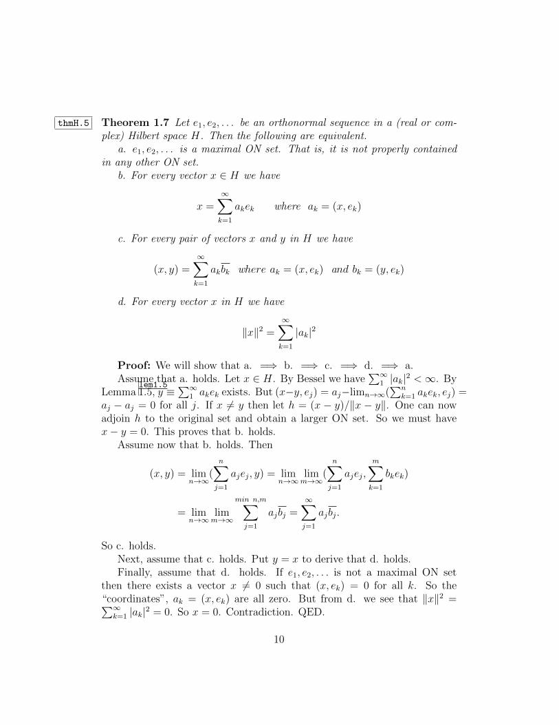
thmH.5 Theorem 1.7 Let e1, e2, . . . be an orthonormal sequence in a (real or com-plex) Hilbert space H. Then the following are equivalent.

a. e1, e2, . . . is a maximal ON set. That is, it is not properly containedin any other ON set.

b. For every vector x ∈ H we have

x =∞∑k=1

akek where ak = (x, ek)

c. For every pair of vectors x and y in H we have

(x, y) =∞∑k=1

akbk where ak = (x, ek) and bk = (y, ek)

d. For every vector x in H we have

‖x‖2 =∞∑k=1

|ak|2

Proof: We will show that a. =⇒ b. =⇒ c. =⇒ d. =⇒ a.Assume that a. holds. Let x ∈ H. By Bessel we have

∑∞1 |ak|2 <∞. By

Lemmalem1.51.5, y ≡

∑∞1 akek exists. But (x−y, ej) = aj−limn→∞(

∑nk=1 akek, ej) =

aj − aj = 0 for all j. If x 6= y then let h = (x − y)/‖x − y‖. One can nowadjoin h to the original set and obtain a larger ON set. So we must havex− y = 0. This proves that b. holds.

Assume now that b. holds. Then

(x, y) = limn→∞

(n∑j=1

ajej, y) = limn→∞

limm→∞

(n∑j=1

ajej,

m∑k=1

bkek)

= limn→∞

limm→∞

min n,m∑j=1

ajbj =∞∑j=1

ajbj.

So c. holds.Next, assume that c. holds. Put y = x to derive that d. holds.Finally, assume that d. holds. If e1, e2, . . . is not a maximal ON set

then there exists a vector x 6= 0 such that (x, ek) = 0 for all k. So the“coordinates”, ak = (x, ek) are all zero. But from d. we see that ‖x‖2 =∑∞

k=1 |ak|2 = 0. So x = 0. Contradiction. QED.

10

Now we’re ready for the definition of ON basis.Definition. An ON sequence {e1, e2, . . . } in a Hilbert space H is an ON

basis of H if condition b. in TheoremthmH.51.7 holds.

Of course we could have used any of the other conditions in TheoremthmH.51.7

for the definition of ON basis because they’re equivalent. So why did I usecondition b. for the definition? Because surveys of your predecessors showthat it’s the most popular.

11

1.3 Problems on Hilbert space

1. Let f1, f2, . . . , f9 be an orthonormal set in L2(0, 1). Assume that

(A)

∫ 1

0

6xf1(x)dx = 2 and

(B)

∫ 1

0

6xf2(x)dx = 2√

2

What can you say about the value of∫ 1

0

6xf5(x)dx?

Give reasons.

2. Letu1(x) = 1/

√2, −1 ≤ x ≤ 1

and

u2(x) =

√3

2x, −1 ≤ x ≤ 1.

Suppose that f and g are in L2([−1, 1]) and ‖f − g‖ ≤ 5. Let aj =∫ 1

−1

uj(x)f(x)dx, j = 1, 2 and bj =

∫ 1

−1

uj(x)g(x)dx. Show that2∑j=1

|aj −

bj|2 ≤ 25. Cite any theorem you use.

3. Suppose that f : [−1, 1]→ R satisfies∫ 1

−1

|f(x)|2dx = 21

and ∫ 1

−1

f(x)dx = 6.

What can you say about the size of∫ 1

−1xf(x)dx?

4. Suppose that u1, u2 are O.N. vectors in an inner product space H. Letf ∈ H and assume that

‖f‖2 = |a1|2 + |a2|2

where aj = (f, uj) for j = 1, 2. Show that f = a1u1 + a2u2.

12

5. The Hermite polynomials are the sequence of polynomials Hn(x)uniquely determined by the properties:

a) Hn(x) is a real polynomial of degree n, n = 0, 1, 2, . . . with positiveleading coefficient.

b) The functions

un(x) = Hn(x)e−x2/4

form an O.N. sequence in L2(R).

Fact that you may use: If f is in L2(R) and

∫ ∞−∞

f(x)un(x)dx = 0 for

n = 0, 1, 2, . . . then f = 0.

Let cn =

∫ ∞−∞

e−|x|un(x)dx.

Evaluate∞∑n=0

c2n.

6. Let {f1, f2, . . .} be an O.N. set in a Hilbert space H. Prove that it isan O.N. basis if and only if the finite linear combinations

n∑j=1

ajfj (n finite but arbitrary)

are dense in H.

7. Let {f1, f2, . . .} be an O.N. set in a Hilbert space H. Prove that it is anO.N. basis if and only if Parseval’s equality

‖g‖2 =∞∑j=1

|(fj, g)|2

holds for a dense set of g in H.

8. Suppose that {f1, f2, . . .} is an O.N. basis of a Hilbert space H andthat {g1, g2, . . .} is an O.N. sequence in H. Suppose further that

∞∑j=1

‖gj − fj‖2 < 1.

Prove that {g1, g2, . . .} is also an O.N. basis.Hint: Use Theorem

thmH.51.7 by supposing that there exists h 6= 0 such that

(h, gj) = 0 for all j.

13

2 Generalized functions. (δ functions and all

that.)

2.1 Dual spaces

The concept of a dual space arises naturally in differential geometry, mechan-ics and general relativity. And we will need it later to understand generalizedfunctions.

Definition 5.1 Let V be a real or complex vector space. A function L :V → scalars is called a linear functional if

L(αx+ βy) = αL(x) + βL(y)

for all x and y in V and for all scalars α and β. In other words a linearfunctional is a linear transformation from V into R (or C if V is a complexvector space.) The dual space to V is the set, denoted V ∗, of all linearfunctionals on V .

For example the function which is identically 0 is a linear functional.(Check this against the definition.) Moreover if L1 and L2 are linear func-tionals then so is the function aL1 + bL2 for any scalars a and b. (Check thisagainst the definition now!) Therefore V ∗ is itself a vector space. Its a newvector space constructed from the old one.

Example 5.2. Denote by P3 the vector space consisiting of polynomialsof degree less or equal to 3. This is a four dimensional vector space because{1, t, t2, t3} constitutes a basis. Here are some linear functionals on this space.

1. p 7→ L1(p) = p(7).

2. p 7→ L2(p) =∫ 1

0p(t)dt.

3. p 7→ L3(p) =∫ 5

0p(t) sin tdt.

[It would be best if you, personally, verify that each of these functions onP3 are linear functionals.]

The thing to take away from these examples is that there is no resem-blance between V and V ∗: you cannot really “identify” any of these threelinear functionals on P3 with elements of P3 itself. RIGHT? V ∗ is really adifferent vector space from V itself. We have constucted a new vector spacefrom the given one. This being the case, you have to regard the followingtheorem as remarkable.

14

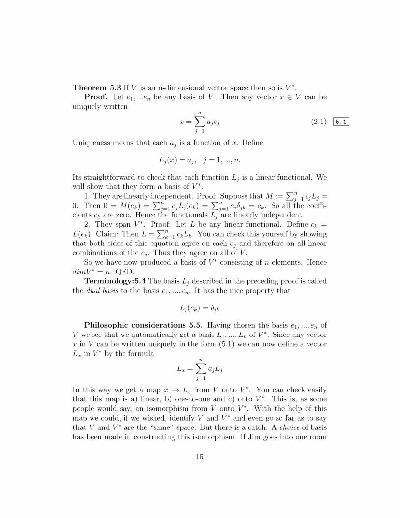
Theorem 5.3 If V is an n-dimensional vector space then so is V ∗.Proof. Let e1, ...en be any basis of V . Then any vector x ∈ V can be

uniquely written

x =n∑j=1

ajej (2.1) 5.1

Uniqueness means that each aj is a function of x. Define

Lj(x) = aj, j = 1, ..., n.

Its straightforward to check that each function Lj is a linear functional. Wewill show that they form a basis of V ∗.

1. They are linearly independent. Proof: Suppose thatM :=∑n

j=1 cjLj =0. Then 0 = M(ek) =

∑nj=1 cjLj(ek) =

∑nj=1 cjδjk = ck. So all the coeffi-

cients ck are zero. Hence the functionals Lj are linearly independent.2. They span V ∗. Proof: Let L be any linear functional. Define ck =

L(ek). Claim: Then L =∑n

k=1 ckLk. You can check this yourself by showingthat both sides of this equation agree on each ej and therefore on all linearcombinations of the ej. Thus they agree on all of V .

So we have now produced a basis of V ∗ consisting of n elements. HencedimV ∗ = n. QED.

Terminology:5.4 The basis Lj described in the preceding proof is calledthe dual basis to the basis e1, ..., en. It has the nice property that

Lj(ek) = δjk

Philosophic considerations 5.5. Having chosen the basis e1, ..., en ofV we see that we automatically get a basis L1, ..., Ln of V ∗. Since any vectorx in V can be written uniquely in the form (5.1) we can now define a vectorLx in V ∗ by the formula

Lx =n∑j=1

ajLj

In this way we get a map x 7→ Lx from V onto V ∗. You can check easilythat this map is a) linear, b) one-to-one and c) onto V ∗. This is, as somepeople would say, an isomorphism from V onto V ∗. With the help of thismap we could, if we wished, identify V and V ∗ and even go so far as to saythat V and V ∗ are the “same” space. But there is a catch: A choice of basishas been made in constructing this isomorphism. If Jim goes into one room

15

and chooses a basis e1, ..., en to construct this isomorphism and Jane goesinto another room and chooses a basis the chances are that they will choosedifferent bases. Then they will arrive at different isomorphisms. So eachone will identify V with V ∗ in different ways. Jim will say that the vectorx ∈ V corresponds to a certain linear functional L and Jane will say, no, itcorresponds to a different linear functional, M .

When an isomorphism between two vector spaces depends on someone’schoice of a basis we say that the isomorphism is not natural. If you shouldnevertheless decide to think of these two vector spaces as the “same” (i.e.identify them) then sooner or later you will run into conceptual and evencomputational trouble.

But there is an important circumstance in which one really can justifyidentifying V and V ∗. (Some readers might recognize the next theorem as“raising and lowering” indices.)

Theorem 5.6. Suppose that V is a real finite dimensional vector spaceand (·, ·) is a given inner product on V . Then for any linear functional L onV there is a unique vector y in V such that

L(x) = (x, y) for all x ∈ V.

Denote by Ly the linear functional determined by y in this way. That is,

Ly(x) = (x, y) for all x ∈ V. (2.2) 5.10

Then the mapy 7→ Ly

is a one-to-one linear map of V onto V ∗. (I.e. it is an isomorphism.)Proof. The map y 7→ Ly is clearly linear. (You better check this. It will

be good practice in dealing with these structures.) Moreover this map is one-to-one because if Ly = 0 then in particular Ly(y) = 0. That is, (y, y) = 0.So y = 0. Therefore the map y 7→ Ly is one-to-one. Hence, by the ranktheorem, the range of this map has the same dimension as the domain. Butif dim V = n then by Theorem 5.3 dim V ∗ = n also. Hence the range is allof V ∗. QED.

Moral 5.7. We know that there are many inner products on any finitedimensional vector space. But given a particular inner product on a realfinite dimensional vector space V , the preceding theorem provides a naturalway to identify V with V ∗ without making any ad hoc choices of basis. Hereis a consequence of this identification that we live with every day.

16

Derivative versus gradient. Suppose that V is a finite dimensionalreal vector space and f is a real valued function on V . For any point x in Vand any vector v ∈ V define

∂vf(x) =df(x+ tv)

dt|t=0

This is the derivative of f in the direction v. For example if we choose anybasis e1, ..., en of V we may write x =

∑nj=1 xjej and then f is just a function

of n real variables, x1, ..., xn. The chain rule then gives

∂vf(x) =n∑j=1

vj(∂f/∂xj)(x)

where of course v =∑n

j=1 vjej. This sum is clearly linear in v. In otherwords the map v → ∂vf(x) is, for each x, a linear functional on V . Oneoften writes f ′(x) for this linear functional. That is, f ′(x)v = ∂vf(x). Sof ′(x) is in V ∗ for each x ∈ V . Therefore the derivative , f ′, is a functionfrom V into V ∗. If there is no natural way to identify V ∗ with V then thismap to V ∗ is the only object around that captures the notion of derivativethat you’re familiar with. But if V has a given inner product, (·, ·), then wecan identify the linear functional f ′(x) ( for each x) with an element of V .This is the gradient of f . That is,

∇f(x) = f ′(x)

identified to an element of V by Theorem 5.6. Thus

f ′(x)v = ∂vf(x) = (∇f(x), v).

17

2.2 Problems on Linear Functionals

Definition. A linear functional on a real or complex vector space V is a scalarvalued function f on V such that

i) f(αx) = αf(x) for all scalars α and all x ∈ V .and ii) f(x+ y) = f(x) + f(y) for all x and y in V .

Which of the following expressions define linear functionals on the givenvector space?

1. V = R3, x = (x1, x2, x3). Explain why not if you think not.

a) f(x) = x1 + 5x2

b) f(x) = x1 + 4

c) f(x) = x21 + 5x3

d) f(x) = 7

e) f(x) = 0

f) f(x) = sin x2

g) f(x) = x1x2

h) f(x) = x · u where u is a fixed vector and x · u =3∑j=1

xjuj

2. V = C([0, 1]) (real valued continuous functions on [0, 1]).

a) F (ϕ) =

∫ 1

0

ϕ(t)dt for ϕ ∈ C([0, 1])

b) F (ϕ) = ϕ(3/5)

c) F (ϕ) = ϕ(0)

d) F (ϕ) = ϕ(0)2

e) F (ϕ) = ϕ(0)ϕ(1)

f) F (ϕ) =

∫ 1

0

ϕ(t) sin tdt

g) F (ϕ) =

∫ 1

0

ϕ(t)2dt

18

h) F (ϕ) =

∫ 1

0

ϕ(t)2tdt

i) F (ϕ) =

∫ 1

0

(ϕ(t)/√t)dt

j) F (ϕ) =

∫ 1

0

(ϕ(t)/t)dt

k) F (ϕ) =

∫ 1

0

(sinϕ(t))dt

Explain why not if you think not.

3. Let V be the vector space of all finitely non–zero real sequences. [Asequence x = (x1, x2, . . . ) is called finitely non–zero if ∃N 3 xk = 0 for allk ≥ N .] If a = (a1, a2, a3, . . .) is an arbitrary sequence of real numbers let

fa(x) =∞∑j=1

ajxj for x in V. (2.3) 1

a) Show that the series converges for each x in V .

b) Show that fa(x) is a linear function of x.

c) Show that every linear functional on V has the form (1). That is, showthat if f is a linear functional on V then there exists a sequence, a, such thatf(x) = fa(x) ∀ x ∈ V .

d) Show that the sequence a, in part c) is unique.

4. Denote by P2 the space of real valued polynomials of degree less or equalto 2. This is a real vector space of dimension three. (Right?) Define an innerproduct on P2 by

(p, q) =

∫ 1

−1

p(t)q(t)dt.

You have already admitted that the function on P2 defined by L(p) =∫ 2

0p(t) sin tdt is a linear functional. But we also know that every linear

functional is given uniquely by an element of the space P2 with the help ofthe inner product. Thus there is a unique polynomial f of degree at most 2such that

L(p) = (p, f) for all p ∈ P2.

Find f .

19

2.3 Generalized functions

If you want to measure the electric field near some point in space you couldput a small charged piece of cork there and measure the force exerted by thefield on the cork. In this way you have converted the problem of makingan electrical measurement to that of making a mechanical measurement. Ofcourse the force on the cork is a (constant multiple of) an average of the forcesat each point of the cork. If E(x) is the field strength at x and ρ is the chargedistribution on the cork then the net force on the cork is

∫R3E(x)ρ(x)d3x,

in appropriate units. In practice (and even in some theories) it is only theseaverages that you can measure. For example if you really want to measurethe field at a point x by the preceding method you would have to place apoint charge at x. But classical theory shows that the total electric energy ofthe field produced by a point charge is infinite. The notion of a point chargeis therefore at best an idealization. Of course if you know in advance that theelectric field is continuous then you can get better and better approximationsto the value of E(x) by using a sequence of smaller and smaller corks. Inthe classical theory of electomagnetic fields the electric field tends to becontinuous and therefore it makes sense to talk about its value at a point.The quantum theory of eletromagnetic fields, however, recognizes that thereare tremendous fluctuations in the field at very small scales and only theaveraged field has a meaning.

The need for talking only about averages shows up also in measurement oftemperature. A thermometer is clearly measuring the average temperatureover the volume of the little bulb at the bottom. If the temerature variesfrom point to point and is a continuous function of position then you can, inprinciple, measure the temperature at a point by using a sequence of smallerand smaller bulbs. Recall however that a typical small bulb will containon the order of 1022 molecules. In accordance with statistical mechanicsthe temperature at a point of a system has a really questionable meaningbecause temperature is a measure of average kinetic energy of a large bunch ofmolecules. So at an atomic size of scale temperature at a point is meaningless.

A pairing such as∫R3E(x)ρ(x)d3x, between an “extensive” quantity such

as charge (“extensive” means that in a larger volume you have more of thestuff, such as charge, mass, etc.) and an “intensive” quantity, such as theelectric field ( in a larger volume you don’t have more field) occurs often inphysics. The integral is linear in ρ and defines a linear functional on the

20

vector space of test charges. The integral is also linear in E for fixed ρ.We say that the integral is a bilinear pairing between the extensive quantityρ and the intensive quantity E. Such bilinear pairings between two vectorspaces is common. Usually the elements in these dual vector spaces have aphysical interpretation, extensive for one and intensive for the other. (JulianSchwinger, in his book “Sources and Fields” emphasizes the duality betweensources and fields.)

We are going to develop and use this notion of duality between verysmooth functions (test functions) and very “rough” functions (e.g. deltafunctions.) It has proven to be a great simplifying machinery for under-standing partial differential equations as well as Fourier transforms. We aregoing to apply it to both.

The first step is to understand really smooth functions.

Test functions

Lemma 1. Let

f(x) =

{e−1/x for x > 0

0 for x ≤ 0

Then f is infinitely differentiable on the entire real line.Proof: First, recall that et grows faster than any polynomial as t→ +∞.

That is, limt→+∞ p(t)e−t = 0 for any polynomial. Second, you can see by

induction that for x > 0 the nth derivative dne−1/xdxn = pn(1/x)e−1/x forsome polynomial pn. [ Convince yourself with the cases n = 0, 1, 2.] Third,you can see easily that all of the derivatives of f exist at any point otherthan x = 0, and is zero to the left of 0. The only question then is whatshappening at x = 0? Sadly, one must go back to the definition of derivativeto answer this. But its not so hard. If we know that the first n derivativesexist at x = 0 and are zero there then the first and second comments aboveshow that the n+ 1st right hand derivative is

limh↓0

pn(1/h)e−1/h − 0

h− 0= 0

Of course the left hand derivative is clearly zero. So the two sided derivativeexists and is zero. This is the basis for an induction proof. Carry out thecase n = 0 yourself. QED.

Lemma 2 Letφ(x) = f(x)f(1− x)

21

where f is the function constructed in Lemma 1. Then φ is an infinitelydifferentiable function on R with support contained in the interval [0, 1].

Proof:. φ is clearly infinitely differentiable by the repeated applicationof the product rule for derivatives. To see that φ is zero outside the interval[0, 1] draw a picture. QED

Notation. C∞c is the standard notation for the set of infintiely differ-entiable functions with support in a finite interval. One says that thesefunctions have compact support.

We have now constructed one (not identically zero) function in C∞c . Fromthis function its easy to construct lots more. For example the function ψ(x) =3φ(2x+ 7) + 5φ(4x)3 is also in C∞c . By scaling and translating the argumentof φ and taking powers one clearly gets lots of such functions. In FACT thereare so many such functions that they are dense in L2(R). [Remember theconcept of density form the chapter on Hilbert space?] One of the homeworkproblems sketches how to show that any continuous function with compactsupport is a limit of functions in C∞c .

Notation The space C∞c arises so often that it customarily is given aspecial notation:

D ≡ C∞c (R).

The dual space of D is denoted, as usual, D∗.

Terminology An element in D∗ is called a distribution or a generalizedfunction (according to taste).

Examples 1. Suppose that f is a continuous function on R. Define

Lf (φ) =

∫ ∞−∞

f(x)φ(x)dx for φ ∈ D. (2.4) 5.1

Then Lf is a linear functional on D. Notice that even if f increases near ∞(e.g. f(x) = ex

2) the integral makes sense because its really an integral over

some (and in fact any) interval that supports φ. So Lf ∈ D∗.2. Let

Lδ(φ) = φ(0).

Then Lδ is also a linear functional on D. (Clear?) So Lδ ∈ D∗. But thisexample is substantially different from the first one. There is no continuousfunction f , or even discontinuous function f , such that Lδ =

∫∞−∞ f(x)φ(x)dx.

22

3. Its still OK if the function f in Example 1 is not continuous but hasonly some mild singularities. For example if f(x) = 1/|x|1/2 in (

5.12.4) then

the integral still exists for any test function φ. All we need of f is that∫ ba|f(x)|dx < ∞ for any finite interval [a, b]. In particular the function

f(x) = 1/|x| won’t work in (5.12.4). The integral doesn’t make sense for an

arbitrary test function φ. One says that f is locally integrable if∫ ba|f(x)|dx <

∞ for any finite interval [a, b].The lesson to be drawn from these examples is this: any continuous

function f on R produces a “generalized function” Lf , i.e. an element ofD∗ by means of the formula (

5.12.4). But not every element of D∗ comes from

a continuous function in this way (or even from a discontinuous function),as we see in Example 2. That’s why we call the elements of D∗ generalizedfunctions. Neat terminology, huh?

4. There is an important instance that violates the wisdom of Example3. Its based strongly on cancellation of singularity.

Lemma Let φ ∈ D. Then

P (1

x)(φ) ≡ lim

a↓0

∫|x|>a

φ(x)

xdx (2.5) 5.3

exists and is equal to∫|x|>1

φ(x)

xdx+

∫ 1

−1

φ(x)− φ(0)

xdx (2.6) 5.4

Proof: If 0 < a < b then∫|x|>a

φ(x)

xdx =

∫|x|>b

φ(x)

xdx+

∫a<|x|≤b

φ(x)− φ(0)

xdx (2.7) 5.5

because∫a<|x|≤b

1xdx = 0. The integrand in the last term in (

5.52.7) is bounded

on R by the mean value theorem. So we can let a ↓ 0 and get a limit. Thisalso proves the validity of the representation (

5.42.6) of this limit. QED

The generalized function P ( 1x) is called the Principal Part of 1/x. It

arises in many contexts. We will see it coming up later in the Feynmanpropagator.

23

2.4 Derivatives of generalized functions

Definition Let T ∈ D∗. The derivative of T is the element T ′ of D∗ givenby

T ′(φ) = −T (φ′) for all φ ∈ D. (2.8) D1

What does this definition have to do with our well known notion of deriva-tive of a function? First lets observe that at least T ′ is indeed a well definedlinear functional on D. The reason is that for any φ ∈ D the function φ′ isagain in D so the right side of (

D12.8) makes sense. The linearity of T ′ is clear.

Right? To understand why this definition is justified consider the exampleT = Lf spelled out in (

5.12.4). Suppose that f is actually differentiable in the

classical sense. (i.e. in the sense that you grew up with.) Then

Lf ′(φ) =

∫ ∞−∞

f ′(x)φ(x)dx

=

∫ b

a

f ′(x)φ(x)dx

where a and b are chosen so that φ = 0 off (a, b)

= f(x)φ(x)|ba −∫ b

a

f(x)φ′(x)dx

= −∫ b

a

f(x)φ′(x)dx

= −∫ ∞−∞

f(x)φ′(x)dx

= −Lf (φ′)

SoLf ′(φ) = −Lf (φ′). (2.9) D3

Stare at (D12.8) and (

D32.9). Do you see now why (

D12.8) is a justifiable definition

of derivative of a generalized function T? That’s right. It agrees with theclassical notion of derivative when T = Lf and f is itself differentiable!!!But (

D12.8) has a well defined meaning even when its not of the form Lf for

some differentiable function f . Lets see what the definition (D12.8) gives when

T = LH and H is the non-differentiable function given by

H(x) =

{1, x ≥ 0

0, x < 0(2.10)

24

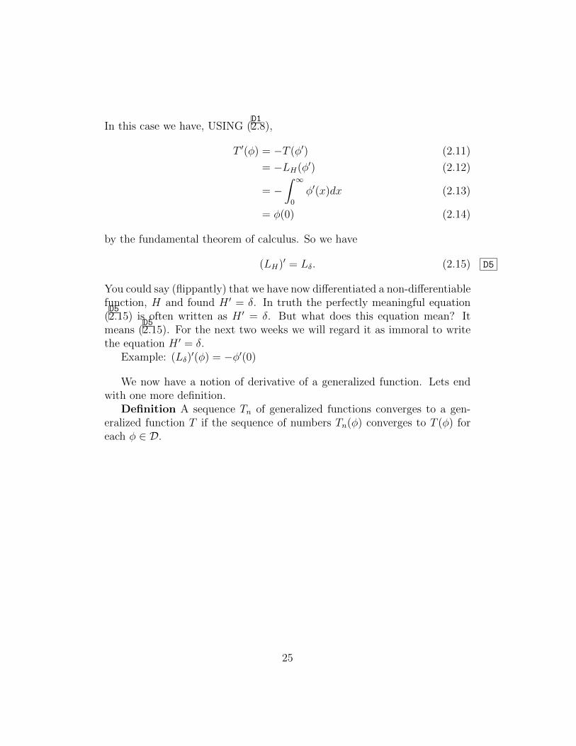
In this case we have, USING (D12.8),

T ′(φ) = −T (φ′) (2.11)

= −LH(φ′) (2.12)

= −∫ ∞

0

φ′(x)dx (2.13)

= φ(0) (2.14)

by the fundamental theorem of calculus. So we have

(LH)′ = Lδ. (2.15) D5

You could say (flippantly) that we have now differentiated a non-differentiablefunction, H and found H ′ = δ. In truth the perfectly meaningful equation(D52.15) is often written as H ′ = δ. But what does this equation mean? It

means (D52.15). For the next two weeks we will regard it as immoral to write

the equation H ′ = δ.Example: (Lδ)

′(φ) = −φ′(0)

We now have a notion of derivative of a generalized function. Lets endwith one more definition.

Definition A sequence Tn of generalized functions converges to a gen-eralized function T if the sequence of numbers Tn(φ) converges to T (φ) foreach φ ∈ D.

25

2.5 Problems on derivatives and convergence of distri-butions.

1. Define

L(φ) =

∫ ∞−∞|x|φ(x)dx for φ ∈ C∞c (R).

Using the definitionT ′(φ) = −T (φ′),

compute the first four derivatives of L; that is, compute T ′, ..., T (4).Hint #1. Use the definition of derivative of a distribution.Hint #2. Use the definition four times to compute the four derivatives.

2. Suppose that f : R→ R is continuous (but not necessarily differentiable.)Let

u(x, t) = f(x− ct).Show that u is a solution to the wave equation

∂2u/∂t2 = c2∂2u/∂x2

in the distribution sense (sometimes called the weak sense.)Nota Bene: Since f is not necessarily differentiable you cannot use f ′ in

the classical sense.

3. Does∑∞

n=1 δ(x− n) converge in the distribution sense?

4. Let pt(x) = (2πt)−1/2e−x2/(2t). Find the folowing limits if they exist.

a. the pointwise limit as t ↓ 0.b. the L2(R) limit.c. the limit in D∗.You may use the following FACT that will be proved later∫ ∞

−∞pt(x)dx = 1 ∀t > 0.

5. Let φ be the function constructed in Lemma 2, except multiply it by apositive constant such that ∫

Rφ(x)dx = 1

26

Such a constant can be found because the original φ is nonnegative and hasa strictly positive integral. Then let

φn(x) = nφ(nx)

Our goal is to show that φn converges in some sense to a delta function.a. Show that

∫R φn(x)dx = 1 for all positive integers n.

b. Suppose that g is a continuous function on R. Show that

limn→∞

∫Rφn(x)g(x)dx = g(0).

c. Use part b. and the definition of convergence of distributions to showthat

Lφn converges in the weak sense to Lδ.

6. Prove that, for all φ ∈ D,

limε↓0

∫ ∞−∞

φ(x)

x+ iεdx = P (

1

x)(φ)− iπφ(0) (2.16) 5.8

This is often written as

limε↓0

1

x+ iε= P (

1

x)− iπδ weak sense (2.17) 5.9

Hint: Review the proof of the lemma at the end of Section 3.3.

27

2.6 Distributions over Rn

The extension of the one dimensional notion of distribution to an n di-mensional distribution is straightforward. Denote by D the vector spaceof infinitely differentiable functions on Rn which are zero outside of a largecube (that can depend on the function.) This space is sometimes denotedC∞c (Rn). There are plenty of such functions. For example if φ1, . . . , φnare each in C∞c (R) then the function ψ(x1, . . . , xn) = φ(x1) · · ·φ(xn) is inC∞c (Rn). (What cube could you use?) So is any finite linear combination ofthese products. A distribution over Rn is defined as a linear functional onD. Of course we can make up examples of such n-dimensional distributionssimilar to the ones we already know in one dimension: Let

Lf (φ) =

∫Rn

f(x)φ(x)dnx (2.18)

As long as |f | has a finite integral over every cube this expression makessense and defines a linear functional on D, just as in one dimension. We alsohave the n-dimensional δ “function” defined by

Lδ(φ) = φ(0). (2.19)

The difference from one dimension shows up when we consider differentiation.We now have partial derivatives. Here is the definition of partial derivative(as if you couldn’t guess).

∂T

∂xk(φ) = −T (∂φ/∂xk). (2.20)

When n = 3 every distribution has a very intuitive interpretation as anarrangement of charges, dipoles, quadrupoles, etc. I’m going to explain thisinterpretation in class in more detail. It gives physical meaning to everyelement of D∗!!!

28

2.7 Poisson’s Equation

We will write as usual r = |x| in R3.

Theorem 2.1

∆1

r= −4πδ. (2.21) P1

in the distribution sense. That is,

∆L1/r = −4πLδ

We will break the proof up into several small steps.

Lemma 2.2 At r 6= 0∆(1/r) = 0

Proof. ∂(1/r)/∂x = −x/r3 and ∂2(1/r)/∂x2 = −1/r3 + 3x2

r5. So

∆(1/r) = −3/r3 + 3x2 + y2 + z2

r5= −3/r3 + 3/r3 = 0.

QED.In view of this lemma you can see that we have only to deal now with

the singularity at r = 0. Our notion of weak derivative is just right for doingthis.

The trick is to avoid the singularity until after one does some cleverintegration by parts (in the form of the divergence theorem). In case youforgot your vector calculus identities a self contained review is at the end ofthis section. I want to warn you that this is not the kind of proof that youare likely to invent yourself. But the techniques are so frequently occurringthat there is some virtue in following it through at least once in one’s life.

Lemma 2.3 Let φ ∈ D. Then∫R3

(1/r)∆φ(x)dx = limε→0

∫r≥ε

(1/r)∆φdx

29

Proof: The difference between the left and the right sides before taking thelimit is at most (use spherical coordinates in the next step)

|∫r≤ε

(1/r)∆φd3x| ≤ maxx∈R3|∆φ(x)|

∫r≤ε

(1/r)d3x = maxx∈R3|∆φ(x)|2πε2 → 0

QED.Before really getting down to business lets apply the definitions.

∆T1/r(φ) =3∑j=1

(∂2/∂x2j)T1/r(φ) (2.22)

= −3∑j=1

(∂/∂xj)T1/r(∂φ/∂xj) (2.23)

= T1/r(∆φ) (2.24)

=

∫R3

(1/r)∆φ(x)d3x (2.25)

= limε→0

∫r≥ε

(1/r)∆φ(x)d3x. (2.26)

So what we really need to do is show that this limit is −4πφ(0). To this endwe are going to apply some standard integration by parts identities in the“OK” region r ≥ ε.

Cε :=

∫r≥ε

(1/r)∆φ(x)d3x (2.27)

=

∫r≥ε∇ ·(1

r∇φ− φ∇(

1

r))d3x by identity (

P82.39) (2.28)

=

∫r=ε

(1

r∇φ · n− φ(∇1

r) · n)dA by the divergence theorem (2.29)

where n is the unit normal pointing toward the origin. The other boundaryterm in this integration by parts identity is zero because we can take it overa sphere so large that φ is zero on and outside it.

30

Now

|∫r=ε

(1/r)(∇φ · n)dA| = 1

ε|∫r=ε

(∇φ · ndA| (2.30)

≤ 1

ε(max |∇φ|)4πε2 (2.31)

→ 0 (2.32)

as ε ↓ 0. This gets rid of one of the terms in Cε in the limit. For the otherone just note that (∇1

r) · n = −∂(1/r)/∂r = 1/r2. So

−∫r=ε

φ(∇1

r) · n)dA = − 1

ε2

∫r=ε

φ(x)dA (2.33)

= − 1

ε2

∫r=ε

φ(0)dA− 1

ε2

∫r=ε

(φ(x)− φ(0))dA (2.34)

= −4πφ(0)− 1

ε2

∫r=ε

(φ(x)− φ(0))dA (2.35)

Only one more term to get rid of!

1

ε2|∫r=ε

(φ(x)− φ(0))dA| ≤ max|x|=ε|φ(x)− φ(0)| · 4π → 0

because φ is continuous at x = 0. This proves (P12.21).

Vector calculus identities.If f is a real valued function and G is a vector field, both defined on some

region in R3 then∇ · (fG) = (∇f) ·G+ f∇ ·G (2.36) P5

Application #1. Take f = 1/r and G = ∇φ. Then we get

∇ · (1

r∇φ) = (∇1

r) · ∇φ+

1

r∆φ wherever r 6= 0. (2.37) P6

Application #2. Take f = φ and G = ∇1r. Then we get

∇ · (φ∇1

r) = (∇φ) · (∇1

r) + φ∆

1

rwherever r 6= 0 (2.38) P7

But ∆1r

= 0 wherever r 6= 0. So subtracting (P72.38) from (

P62.37) we find

1

r∆φ = ∇ · (1

r∇φ− φ∇1

r) wherever r 6= 0. (2.39) P8

This is the identity we need in the proof of (P12.21).

31

3 The Fourier Transform

The Fourier transform of a complex valued function on the line is

f(ξ) =

∫ ∞−∞

eiξxf(x)dx (3.1) F1

Here ξ runs over R. The most useful aspect of this transform of functions isthat it interchanges differentiation and multiplication. Thus if you differen-tiate under the integral sign you get

d

dξf(ξ) =

∫ ∞−∞

eiξx{ixf(x)}dx. (3.2) F2

So

(Fourier transform of{ixf(x)})(ξ) =d

dξf(ξ). (3.3)

And an integration by parts (never mind the boundary terms) clearly gives

−iξf(ξ) =

∫ ∞−∞

eiξxf ′(x)dx. (3.4) F3

Sof ′(ξ) = −iξf(ξ) (3.5)

We will see later that these formulas allow one to solve some partial differen-tial equations. Moreover in quantum mechanics these two formulas amountto the statement that the Fourier transform interchanges P and Q (momen-tum and position operators.)

But the usefulness of these formulas depends crucially on the fact thatone can also transform back and recover f from f . To this end there is aninversion formula that does the job. Our goal is to establish the most usefulproperties of the Fourier transform and in particular to derive the inversionformula and show how to use it to solve PDEs.

To begin with we must understand how to give honest meaning to theformula (

F13.1). Since the integral is over an infinite interval there is a conver-

gence question right away. Suppose that∫ ∞−∞|f(x)|dx <∞. (3.6) F4

32

We will write f ∈ L1 if (F43.6) holds. If f ∈ L1 then there is no problem with

the existence of the integral in (F13.1) because lima→∞

∫ a−a e

iξxf(x)dx exists.

[Proof: |( ∫ a−a−

∫ b−b

)eiξxf(x)dx| ≤

∫a≤|x|≤b |f(x)|dx→ 0 as a ≤ b→∞. Use

the Cauchy convergence criterion now.]Of course even if f ∈ L1 it can happen that f ′ is not in L1 and/or that

xf(x) is not in L1. This is a nuisance in dealing with the identities (F23.2) and

(F33.4). We are going to restrict our attention for a while to a class of functions

that will make these issues easy to deal with.Definition. A function f on R is said to be rapidly decreasing if

|xnf(x)| ≤Mn, n = 0, 1, 2, ... (3.7) F5

for some real numbers Mn. In words: xnf(x) is bounded on R for each n.Examples 1. e−x

2is rapidly decreasing.

2. 1x2+1

is not rapidly decreasing because (F53.7) only holds for n = 0, 1, 2

but not for n = 3 or more.3. If f is rapidly decreasing then so is x5f(x) because xnx5f(x) =

xn+5f(x) which is bounded in accordance with (F53.7). Just replace n by n+ 5

in (F53.7). Since any finite linear combination of rapidly decreasing functions

is also rapidly decreasing we see that p(x)f(x) is rapidly decreasing for anypolynomial p if f is rapidly decreasing.

4. So by examples 1. and 3. we see that p(x)e−x2

is rapidly decreasingfor any polynomial p.

5. Any function in C∞c (R) is rapidly decreasing.6. Summary: The space of rapidly decreasing functions is a vector space

and is closed under multiplication by any polynomial. And besides, there arelots of these functions.

Lemma Any rapidly decreasing function is in L1.Proof: Apply (

F53.7) for n = 0 and n = 2 to conclude that

|(1 + x2)f(x)| ≤M

for some real number M . So∫ ∞−∞|f(x)|dx ≤M

∫ ∞−∞

1

x2 + 1dx <∞.

QEDUsing only rapidly decreasing functions in (

F23.2) will allow us not to have

to worry about whether f and xf(x) are both in L1. Neat, huh?

33

But to use (F33.4) we still need to worry about whether f ′ is in L1. So

we are going to restrict our attention for a while, even further, to a class offunctions that makes both (

F23.2) and (

F33.4) easy to deal with.

Notation: S will denote the set of C∞ functions on R such that f andeach of its derivatives is rapidly decreasing.

Examples7. e−x

2is infinitely differentiable and each derivative is just a polynomial

times e−x2. We’ve already seen that these functions are rapidly decreasing.

So the function e−x2

is in S.8. 1

x2+1is infinitely differentiable but is not rapidly decreasing. So this

function is not in S.9. Now here is a real nice thing about this space S. If f ∈ S then any

polynomial, p, times any derivative of f is again in S. CHECK THIS againstthe definitions! I know this may seem too good to believe. But we do knowthat there are lots of functions in S. All of C∞c is contained in S. Andbesides there are more, as we saw in Example 7.

STATUS: If f ∈ S then f and all of its derivatives are in L1. So bothformulas (

F23.2) and (

F33.4) make sense. Moreover they are both correct because

the boundary terms that we ignored in deriving (F33.4) are indeed zero, since

these functions go to zero so quickly at ∞. (Check this at your leisure!)In truth, here is the reason that the space S is so great.Invariance Theorem. If f ∈ S then f ∈ S.Proof: First notice that for any function f in L1 we have the bound

|f(ξ)| = |∫ ∞−∞

eiξxf(x)dx| (3.8)

≤∫ ∞−∞|f(x)|dx (3.9)

= ‖f‖1. (3.10)

Since the right side doesn’t depend on ξ f is bounded.Now suppose that f ∈ S. Then so is f ′, f ′′, etc. So f ′, f ′′ etc. are all

in L1. By (F33.4) it now follows that ξnf(ξ) is bounded for each n = 0, 1, 2....

So f is rapidly decreasing. But df(ξ)/dξ is the Fourier transform of ixf(x)which we have seen is also in S. So df(ξ)/dξ is also rapidly decreasing. Andso on. QED.

34

Here is what the inversion formula will look like

f(y) =1

2π

∫ ∞−∞

e−iyξf(ξ)dξ. (3.11) F8

Since we already know that f is in S we know that the right hand side of(F83.11) makes sense. Contrast this with the example that you worked out in

the homework: Take f(x) = 1 if |x| ≤ 1 and f = 0 otherwise. Then f ∈ L1

so f makes sense. But f itself decreases so slowly at∞ that its not in L1. So(F83.11) doesn’t make sense. Aren’t you glad that we are focusing on functions

in S?Notation:

g(y) =1

2π

∫ ∞−∞

e−iyξg(ξ)dξ (3.12) F9

Inversion Theorem. For f ∈ S equation (F83.11) holds.

In other words :ˇf = f .

We are going to spend the next few pages proving this formula. (Notbecause I fear that you might not trust me, but because the proof derivessome very useful identities along the way.)

35

3.1 The Fourier Inversion formula on S(R).

To begin, here are some explicit computations of some important Fouriertransforms.

Gaussian identitiesLet

pt(x) =1√2πt

e−x2/2t (3.13) F10

Then we have the following three identities.∫ ∞−∞

pt(x)dx = 1 (3.14) F11

pt(ξ) = e−tξ2/2 (3.15) F12

ˇ(e−

t2ξ2)(x) =

1√2πt

e−x2/2t = pt(x). (3.16) F13

Proof of (F113.14) [Sneaky use of polar coordinates.]

{∫ ∞−∞

pt(x)dx}2 =

∫R2

pt(x)pt(y)dxdy (3.17)

=1

2πt

∫R2

e−x2+y2

2t dxdy (3.18)

=1

2πt

∫ ∞0

∫ 2π

0

e−r2/2trdrdθ (3.19)

= 1 (3.20)

(Use the substitution s = r2/(2t) in the last step.)

Proof of (F123.15)

To compute pt(ξ) we need first to multiply pt(x) by eixξ before integration.The exponent is a quadratic function of x for which we can complete thesquare thus:

−x2

2t+ ixξ = − 1

2t(x− itξ)2 − tξ2/2

Hence

pt(ξ) = e−tξ2/2 1√

2πt

∫ ∞−∞

e−12t

(x−itξ)2dx (3.21) F16

36

The coefficient of e−tξ2/2 looks “just like”

∫∞−∞ pt(x)dx which is one. This

would prove (F123.15). But not so fast. x has been translated by the imaginary

number itξ. You can’t just translate the argument to get rid of it. Hereis how to get rid of it. Let a = −tξ. and suppose a > 0 just so that Ican draw pictures verbally. Take a large positive number R and considerthe rectangular contour in the complex plane which starts at −R on thereal axis, moves along the real axis to R and then moves vertically up tothe point R + ia. From there move horizontally, west to −R + ia and thensouth back to the point −R. Since e−z

2/(2t) is an entire function, the integralof this function around this rectangular contour is zero. Otherwise put,∫ R−R e

(x+ia)2/(2t) =∫ R−R e

−x2/(2t)dx plus a little contribution from the verticalsides of the rectangle. On the right end the integral is at most a timesthe maximum value of the integrand on that segment. But |e−(R+iy)2/(2t)| =e(−R2+y2)/(2t), which goes to zero quite quickly for 0 ≤ y ≤ a as R →∞. Sothe integrals along the end segments go to zero as R → ∞. So it is indeedtrue that the coefficient of e−tξ

2in (

F163.21) equals

∫∞−∞ pt(x)dx, which is one.

QED

Proof of (F133.16) e−tξ

2/2 =√

2πtp1/t(ξ) by (

F103.13). Since p1/t is even we have

(e−tξ2/2) = (1/2π)

√2πt

(p1/t)(x) = 1√2πte−x

2/2t by (F123.15). QED

Definition 3.1 The convolution of two functions f and g on R is given by

(f ∗ g)(x) =

∫R

f(x− y)g(y)dy (3.22) F21

lemF1 Lemma 3.2 Let g be a bounded continuous function on R. Then for each x

limt↓0

(pt ∗ g)(x) = g(x).

Proof: Since∫∞−∞ pt(x)dx = 1 we have

(pt ∗ g)(x)− g(x) = (g ∗ pt)(x)− g(x) (3.23)

=

∫g(x− y)pt(y)dy − g(x) (3.24)

=

∫ ∞−∞

(g(x− y)− g(x))pt(y)dy. (3.25)

37

Given ε > 0, ∃ δ > 0 3 |g(x− y)− g(x)| < ε if |y| < δ.

∴ |pt ∗ g(x)− g(x)| ≤∫ δ

−δ|g(x− y)− g(x)|pt(y)dy (3.26)

+

∫|y|>δ|g(x− y)− g(x)|pt(y)dy (3.27)

≤ ε

∫ δ

−δpt(y)dy + 2|g|∞

∫|y|>δ

pt(y)dy (3.28)

≤ ε+ 2|g|∞∫|y|>δ

pt(y)dy. (3.29)

∴ limt↓0|(pt ∗ g)(x)− g(x)| ≤ ε+ 2|g|∞lim

t↓0

∫|y|≥δ

pt(y)dy.

But∫y≥δ

pt(y)dy =2√2πt

∫ ∞δ

e−y2/2tdy ≤ 2√

2πt

∫ ∞δ

y

δe−y

2/2tdy (3.30)

=2

δ√

2πt[−te−y2/2t]∞δ =

2

δ√

2π

√te−δ

2/2t → as t ↓ 0. (3.31)

Thereforelimt↓0|(pt ∗ g)(x)− g(x)| ≤ ε ∀ ε > 0.

Hencelimt↓0|(pt ∗ g)(x)− g(x)| = 0.

Q.E.D.

Lemma 3.3 If f and g are in S(R) then

(f ∗ g)(x) =1

(2π)n

∫f(ξ)e−iξ·xg(ξ).

38

Proof:

(f ∗ g)(x) =

∫R

f(x− y)g(y)dy (3.32)

=1

(2π)n

∫R

∫R

f(ξ)e−iξ·(x−y)g(y)dξdy (3.33)

=1

(2π)n

∫R

∫R

f(ξ)e−iξ·xeiξ·yg(y)dydξ (3.34)

=1

(2π)n

∫R

f(ξ)e−iξ·xg(ξ)dξ. (3.35)

Q.E.D.

Theorem 3.4 If g is in S(R) then

(g)ˇ(x) = g(x).

Proof. In the preceding lemma put f(ξ) = e−tξ2/2. Then, by (

F133.16), f(x) =

pt(x). Thus

(pt ∗ g)(x) =1

2π

∫R

e−tξ2

e−iξ·xg(ξ)dξ.

Let t ↓ 0. Use LemmalemF13.2 on the left and Dom. Conv. theorem on the right

to get

g(x) =1

2π

∫R

e−iξ·xg(ξ)dξ.

The asymmetric way in which the factor 2π occurs in the inversion formulais sometimes a confusing nuisance. It is useful to distribute this factor amongthe forward and backward transforms. Define

(Fg)(ξ) = (2π)−1/2g(ξ) (3.36)

The factor in front of g has clearly no effect on the one-to-one or ontonessproperty of the map g → g. That is, F is a one-to-one map of S(R) ontoS(R). However the factor makes for a nice identity:

corFPl Corollary 3.5 (Plancherel formula for S) If f and g are in S(R) then

(Ff,Fg) = (f, g) (3.37) F50

39

Explicitly, this says∫R

(Ff)(ξ)(Fg)(ξ)dξ =

∫R

f(x)g(x)dx (3.38)

Proof. Phrasing this identity directly in terms of f and g, it asserts that∫R

f(ξ)g(ξ)dξ = (2π)

∫R

f(x)g(x)dx

But g(ξ) =∫g(x)eix·ξdx =

∫g(x)e−ix·ξdx. Hence∫

R

f(ξ)g(ξ)dξ =

∫R

∫R

f(ξ)g(x)e−ix·ξdxdξ (3.39)

=

∫R

(∫R

f(ξ)e−ix·ξg(x)dξ)dx (3.40)

=

∫R

(2π)f(x)g(x)dx. (3.41)

Q.E.D.

3.2 Extension of the Fourier transform to L2 and otherfunction spaces.

Lemma 3.6 Let V be a dense linear subspace of a Banach space X. Supposethat S : V → Y is a bounded linear operator from V into a Banach space Y .Then there exists a unique bounded linear operator T : X → Y which extendsS.

Proof. Let M = ‖S‖V→Y . Suppose that x ∈ X. Then there exists asequence xn ∈ V such that xn → x. Hence ‖Sxn−Sxk‖Y ≤M‖xn−xk‖V →0. Since Y is complete the Cauchy sequence Sxn has a limit, y. DefineTx = y. Then

1. T is well defined. I.e. it is independent of the choice of Cauchysequence. T and S agree on V . ( I leave these to you to show.)

2. T is linear on X. (You can show this too.)3. ‖T‖ ≤ ‖S‖ and consequently ‖T‖ = ‖S‖. (Ditto).4. The extension T is unique among all bounded linear operators extend-

ing S. (Try your hand at this too.)

40

Theorem 3.7 The Fourier transform F : S → S has a unique continu-ous extension F : L2(R) → L2(R). Moreover F is one-to-one, onto andisometric.

Proof. Put g = f in (F503.37) to deduce that ‖Ff‖L2 = ‖f‖L2 for all

f ∈ S. Since S is dense in L2(R) the lemma assures us that F has a uniquecontinuous extension F to L2 and in fact ‖F‖L2→L2 = 1. Furthermore, iffn ∈ S and fn → f in L2 norm then (

F503.37) and the proof of the lemma show

that‖Ff‖L2 = ‖f‖L2 for all f ∈ L2. (3.42) F60

So F is an isometry and is therefore automatically one-to-one. Now if gn ∈ L2

and Fgn coverges in L2 to some element h ∈ L2 then Fgn is Cauchy andtherfore, by isometry, gn is also Cauchy and hence has an L2 limit g. Butthen Fg = limFgn = h. So the range of F is a closed subspace of L2. Butthe range of F contains the range of F , which is S and which is itself densein L2. Hence the range of F is all of L2.

Terminology A linear map from one Hilbert space to another whichis one-to-one, isometric, and surjective is called unitary. So the extendedFourier transform F is a unitary operator from L2(R) onto L2(R).

The prescription we’ve used to define F on L2(R) has been rather indirect.Here is a more direct prescription.

Suppose that f ∈ L2(R) and is zero outside the interval [−a, a]. Choosea real number b > a. Then there exists a sequence φn ∈ C∞c (R) such thatall φn are zero outside (−b, b) and converge to f ∈ L2((−b, b)). Since b isfinite we know that f is in L1((−b, b)) and that the sequence converges to fin L1((−b, b)) also. Therefore, for each ξ ∈ R

(2π)1/2(Fφn)(ξ) =

∫ b

−bφn(x)eixξdx

which converges , by the dominated convergence theorem, to∫ b−b f(x)eixξdx,

which, by the way is clearly a continuous function of ξ. But Ff is, by defi-nition, the L2 limit of the sequence Fφn, which we have just seen convergespointwise to

∫ b−b f(x)eixξdx. Hence

(Ff)(ξ) = (2π)−1/2

∫ ∞−∞

f(x)eixξdx (3.43) F66

41

for almost all ξ. (Recall that the left side is just an L2 limit.) Of course wemay take (

F663.43) as the actual function representing the equivalence class on

the left. It is customary to do so and we shall follow this custom.Denote by L2

c(R) the subspace of L2(R) consisting of functions which arezero outside some bounded interval. We have seen that for these functionsFf is just given explicitly by (

F663.43).

Next, let g be an arbitrary function in L2(R). Define gn(x) = g(x)χ(−n,n)(x).Then (

F653.55) holds for gn. But gn converges in L2(R) to g. (Use DCT.) Hence

Fg is the L2 limit of Fgn because F is an isometry ( and hence continuous.)Therefore we may write

(Fg)(ξ) = l.i.m.n→∞

∫ n

−ng(x)eixξdx (3.44) F67

where l.i.m. means “ limit in the L2 sense”, but is translated as “limit inmean”. (

F673.44) is the classical way (early 20th century) of describing the

Fourier transform as a unitary operator on L2(R). You can’t get rid of thatl.i.m. by just writing

∫∞−∞ g(x)eixξdx because the integrand is not in L1(R)

for a general function g ∈ L2(R). For example if g(x) = (1 + |x|)−1 theng ∈ L2 but not in L1. Hence

∫∞−∞ g(x)eixξdx is +∞ at ξ = 0 and yet for

a.e. ξ the integrals in (F673.44) converge as n → ∞. (Of course you may need

to drop down to a subsequence of n.) This results from cancellation in theoscillating integrand. Is that amazing, or what?

We now have specific formulas for Ff for various spaces of functions, asfollows.S, L2

c(R), L2(R), L1 ∩ L∞ (which is contained in L2), and{f ∈ L1 ∩ L∞ ∩ C(R) : f ∈ L1(R)}Given all the information that we have you can now verify that the in-

version formula holds on the last space. Namely

f(x) = (2π)−1

∫Rf(ξ)e−ixξdξ ∀ x ∈ R (3.45) F68

if f ∈ L1 ∩ L∞ ∩ C(R) and f ∈ L1.Exercise: Prove (

F683.45).

42

3.3 The Fourier transform over Rn

The definitions, key formulas, theorems and proofs for the Fourier transformover Rn are nearly identical to those over R. In this section we are going tosummarize the results we’ve obtained so far and formulate them over Rn.

The Fourier transform of a complex valued function on Rn is

f(ξ) =

∫Rn

eiξ·xf(x)dx (3.46) F51

Here ξ runs over Rn. Just as in one dimension, one must pay some attentionto the meaningfulness of this integral. But the ideas are similar.

As in one dimension, the Fourier transform over Rn interchanges multi-plication and differentiation. The analog of (

F23.2) is

∂

∂ξjf(ξ) =

∫Rn

eiξ·x{ixjf(x)}dx. (3.47) F52

So

(Fourier transform of{ixjf(x)})(ξ) =∂

∂ξjf(ξ). (3.48)

An integration by parts (never mind the boundary terms) clearly gives theanalog of (

F33.4):

−iξj f(ξ) =

∫Rn

eiξ·x(∂f/∂xj)(x)dx. (3.49) F53

So∂f/∂xj(ξ) = −iξj f(ξ) (3.50)

We will see later that these formulas allow one to solve some partial differen-tial equations. Moreover in quantum mechanics these two formulas amountto the statement that the Fourier transform interchanges Pj and Qj (mo-mentum and position operators.)

We say that a function f is in L1(Rn) if∫Rn

|f(x)|dnx <∞ (3.51)

The formula (F513.46) makes perfectly good sense if f ∈ L1(Rn). But in

the end we are going to give meaning to (F513.46) for a much larger class of

functions and generalized functions, including e.g. delta functions and theirderivatives. To this end we need the n-dimensional analog of S.

43

Definition 3.8 A function f on Rn is said to be rapidly decreasing if

|x|k|f(x)| ≤Mk, k = 0, 1, 2, ... (3.52) F55

for some real numbers Mk. In words: |x|kf(x) is bounded on Rn for each k.

In Exercise 4 you will have the opportunity to show that the condition(F553.52) is equivalent to the statement that for any polynomial p(x1, . . . , xn)

in n real variables, the product p(x)f(x) is bounded.

lemF20 Lemma 3.9 Any rapidly decreasing function on Rn is in L1(Rn).

Definition 3.10 S(Rn) is the set of functions f in C∞(Rn) such that f andeach of its partial derivatives are rapidly decreasing.

Theorem 3.11 a. If f is in S(Rn) then f is also in S(Rn).b. The map f → f is a one-to-one linear map of S(Rn) onto S(Rn).c. The inverse is given by the inversion formula

f(y) = (2π)−n∫Rn

e−iξ·yf(ξ)dnξ. (3.53) F60

Definition 3.12 The convolution of two functions f and g on Rn is givenby

(f ∗ g)(x) =

∫Rn

f(x− y)g(y)dny (3.54) F61

The important identity in the next theorem is the basis for the applicationof the Fourier transform to solution of partial differential equations.

Theorem 3.13(f ∗ g)(ξ) = f(ξ)g(ξ) (3.55) F65

Proof. The proof consists of the following straight forward computation.A reader who is concerned about the validity of any of these steps should

44

simply assume that f and g are in S(Rn), although the identity is valid quitea bit more generally.

f ∗ g(ξ) =

∫Rn

(f ∗ g)(x)eix·ξdx (3.56)

=

∫Rn

∫Rn

f(x− y)g(y)dyeix·ξdx (3.57)

=

∫Rn

∫Rn

(f(x− y)ei(x−y)·ξ)dxg(y)eiy·ξdy (3.58)

=

∫Rn

f(ξ)g(y)eiy·ξdy (3.59)

= f(ξ)g(ξ) (3.60)

Theorem 3.14 (Plancherel formula) Define Fφ = (2π)−n/2φ. Then

‖Fφ‖L2(Rn) = ‖φ‖L2(Rn) (3.61) F70

This is the Plancherel formula. As a consequence F is a unitary operator onL2(Rn)

This is a minor restatement of CorollarycorFPl3.5 and extension to Rn.

Finally, here are the n-dimensional analogs of the important Gaussianidentities (

F113.14) - (

F133.16).

Gaussian identities over Rn.Let

pt(x) =1√

(2πt)ne−|x|

2/2t x ∈ Rn. (3.62) F80

Then ∫Rn

pt(x)dx = 1 (3.63) F81

pt(ξ) = e−t|ξ|2/2 (3.64) F82

ˇ(e−

t2|ξ|2)(x) =

1√(2πt)n

e−|x|2/2t = pt(x). (3.65) F83

45

3.4 Tempered Distributions

Definition 3.15 A tempered distribution on Rn is a linear functional onS(Rn).

Example 3.16 (n = 1) Suppose that f : R→ C satisfies

|f(x)| ≤ const.(1 + |x|n)for some n ≥ 0 (3.66) F30

In this case we say that f has polynomial growth. E.g. x3 sinx has polynomialgrowth. (Take n = 3 in (

F303.66). Of course n = 4 will also do.) If f has

polynomial growth then the integral

Lf (φ) ≡∫Rf(x)φ(x)dx (3.67) F31

exists when φ ∈ S because |f(x)φ(x)| ≤ const.(1 + |x|n)(1 + |x|n+2)−1, whichgoes to zero at ∞ like x−2 and so is integrable. Clearly Lf is linear. Thusany function of polynomial growth determines in this natural way a linearfunctional on S. Remember that we did not need polynomial growth of fwhen we made Lf into a linear functional on D. So we have a “smaller” dualspace now. But the delta distribution and its derivatives are in this smallerdual space anyway because

Lδ(φ) ≡ φ(0)

is a meaningful linear functional on S. (And similarly for δ(k).)

Example 3.17 We can’t allow the function f(x) = e2x2 in (F313.67) because

the function φ(x) = e−x2

is in S and so (F313.67) wouldn’t make sense.

Definition 3.18 The Fourier transform of an element L ∈ S∗ is defined by

L(φ) = L(φ) for φ ∈ S. (3.68) F33

Now you can see the virtue of using S as our new test function space: theright hand side of (

F333.68) makes sense precisely because φ is back in S when

φ is in S. After all, L is only defined on S. Had we attempted to use D thisdefinition would have failed because φ is never in D when φ ∈ D (if φ 6= 0.)

46

Example 3.19 Lδ = L1. (In the outside world this is usually written δ = 1.

Proof. Let φ ∈ S. Then

Lδ(φ) = Lδ(φ) by def. (F333.68) (3.69)

= φ(0) by the def. of Lδ (3.70)

=

∫Rφ(x)dx by the def. of Fourier trans. at 0 (3.71)

= L1(φ) by yet another definition (3.72)

One thing to take away from this proof is that every step is just theapplication of some definition. There is no mysterious computation. Let thisbe a lesson to all of us!

Example 3.20L1 = 2πLδ (3.73) F40

After you have achieved a suitable state of sophistication you can write thisas

1 = 2πδ.

Or even as!!1

2π

∫ ∞−∞

eixydx = δ(y)

(if you don’t feel too uncomfortable with the seeming nonsense of the leftside. But you better get used to it. Thats how (

F403.73) is written in the

outside world.)

Proof. of (F403.73):

L1(φ) = L1(φ) by def. (F333.68) (3.74)

=

∫Rφ(ξ)dξ by def.of L1 (3.75)

= 2πφ(0) by the Fourier inversion formula (3.76)

Notice that this time the last step uses something deep.

47

Consistency of the two definitions of the Fourier transform. If f ∈ L1

then we already have a meaning for f . So is

Lf = Lf?

Yes. Here is a (definition chasing) proof.

Lf (φ) = Lf (φ) (3.77)

=

∫Rf(ξ)φ(ξ)dξ (3.78)

=

∫Rf(ξ)

∫Reixξφ(x)dxdξ (3.79)

=

∫R

( ∫Rf(ξ)eixξdξ

)φ(x)dx (3.80)

=

∫Rf(x)φ(x)dx (3.81)

= Lf (φ) (3.82)

QED

48

3.5 Problems on the Fourier Transform

1. Find the Fourier transforms of the following functions:

a) e−|x|

b) e−x2/2

c) xe−x2/2

d) x2e−x2/2

e) f(x) =

{1 if a ≤ x ≤ b

0 otherwise.

f)1

1 + x2

2. For ϕ in S(R2) define

T (ϕ) =

∫ ∞−∞

xϕ(x, 0)dx.

(Note that this is an integral over a line — not over R2.)

a) Show that T is in S ′(R2).

b) Find the Fourier transform, T , of T explicitly (explicitly enough to do

part c) without finding ψ).

c) Evaluate T (ψ) where

ψ(ξ, η) =ξe−(ξ2+η2)

1 + ξ2

d) Let L = a∂2

∂ξ2+ b

∂2

∂ξ∂η+ c

∂2

∂η2. Find all values of the real parameters

a, b, c such thatLT = 0.

3. Computea. δ′

b. δ′′

c. Lx

49

d. Lx2Hints: 1. Use the definitions. 2. Use the definitions. 3. Use the

definitions.

4. Show that a function f on Rn is rapidly decreasing if and only if, for everypolynomial p(x1, . . . , xn), the function p(x)f(x) is bounded.

5. Derive the identities (F813.63) - (

F833.65) from the one-dimensional identities

(F113.14) - (

F133.16).

50