MATH 353: ODE AND PDE NOTES PART II

παιδειαs αρχη oνoµατων επισκεψιs

(learning begins with what words mean)

Stephanos Venakides

October 13, 2015

Contents

1 VECTOR SPACES OF FUNCTIONS 3

1.1 The L2 space of periodic functions . . . . . . . . . . . . . . . . . . . . . . . . 7

2 OPERATOR EIGENVALUE PROBLEMS and EIGENFUNCTION EX-

PANSIONS 11

2.1 Orthogonal basis series expansion for solving linear IVP . . . . . . . . . . . . 11

2.1.1 Example/exercise . . . . . . . . . . . . . . . . . . . . . . . . . . . . . 15

2.2 Calculating the eigenfunctions and eigenvalues of L. . . . . . . . . . . . . . 16

2.3 Selfadjointness, reality of eigenvalues and orthogonality of eigenfunctions . . 19

2.4 Diagonalization of the operator L (Optional) . . . . . . . . . . . . . . . . . . 22

3 Derivation of the heat or diffusion equation 25

3.1 Conservation law and flux law. . . . . . . . . . . . . . . . . . . . . . . . . . 25

3.2 Diffusion in nature . . . . . . . . . . . . . . . . . . . . . . . . . . . . . . . . 27

1

4 PARTIAL DIFFERENTIAL EQUATIONS (PDE) 29

4.1 Separation of variables . . . . . . . . . . . . . . . . . . . . . . . . . . . . . . 29

4.2 The heat equation . . . . . . . . . . . . . . . . . . . . . . . . . . . . . . . . 30

4.2.1 Solution of the initial-boundary value problem of the heat equation in

a bounded domain by means of eigenfunction expansions . . . . . . . 30

4.3 The wave equation . . . . . . . . . . . . . . . . . . . . . . . . . . . . . . . . 33

4.3.1 Derivation . . . . . . . . . . . . . . . . . . . . . . . . . . . . . . . . . 33

4.3.2 General solution on the line and the d’Alambert solution formula . . 35

4.3.3 Solution of the initial-boundary value problem for the wave equation

in a bounded domain by means of eigenfunction expansions . . . . . . 37

4.4 The Laplace equation: A boundary value problem (BVP) . . . . . . . . . . . 38

4.4.1 Derivation and significance . . . . . . . . . . . . . . . . . . . . . . . . 38

4.4.2 Solution of the boundary value problem for the Laplace equation by

means of eigenfunction expansions . . . . . . . . . . . . . . . . . . . . 40

4.5 Introduction to dispersive wave equations (the wave equation in one space

dimension is non-dispersive) . . . . . . . . . . . . . . . . . . . . . . . . . . . 43

4.6 Review of the method of eigenfunction expansions . . . . . . . . . . . . . . . 44

4.7 The Fourier transform . . . . . . . . . . . . . . . . . . . . . . . . . . . . . . 46

4.8 PDE applications of Fourier Transform . . . . . . . . . . . . . . . . . . . . . 49

4.8.1 The initial value problem for the Schrodinger Equation on the line . . 49

2

1 VECTOR SPACES OF FUNCTIONS

Vector spaces whose elements are functions (for example the set of all polynomials, or the

set of functions that are periodic with a certain period) are typically infinite-dimensional,

that is, there is no finite set of such functions that constitutes a basis of the vector space. In

this chapter, we examine to what extent basic notions of linear algebra, such as linear combi-

nation, basis, dot product, orthogonality, etc may be extended to these infinite-dimensional

spaces.

We begin by considering all real-valued functions f(x) that are defined on an interval

a ≤ x ≤ b. It is often advantageous to restrict ourselves to these functions that have the

property ∫ b

a

|f(x)|2dx <∞, (1)

i.e., these functions for which the above integral exists1 and is finite. These functions are

referred to as square-integrable on the interval (a, b). They constitute a vector space

that is denoted by L2(a, b).

Our work with functions in L2(a, b) is similar to how we work with vectors in Rn. In

analogy to the dot product of two vectors with real entries u and v,

u · v =n∑i=1

uivi, (2)

we define the inner product of two real valued functions f(x) and g(x) in L2(a, b) by

replacing the summation of the component-wise product of the two vectors, by the integration

of the product of the two functions.

(f, g) =

∫ b

a

f(x)g(x)dx. (3)

1The space includes functions that cannot be integrated in the classic sense taught in calculus (Riemannintegration), but can be integrated in a more subtle sense (Lebesgue integration). Since essentially all thefunctions that we will encounter explicitly are Riemann integrable, we need not dwell on this issue.

3

Same as the dot product of two vectors, the inner product of two functions is a scalar.

Let us first illustrate the analogies between RN and L2(0, L), at the same time defining

orthogonality in L2(0, L).

1. Orthogonality

(a) Vectors in RN :Two vectors u and v in Rn are orthogonal if their dot product

is zero, u · v = 0.

(b) Functions in L2: Two functions f and g in L2(0, L) are orthogonal if their

inner product is zero, (f, g) = 0.

2. Representation as a linear superposition of basis vectors.

(a) Vectors in Rn : Let b1,b2,b3, · · · ,bN be an orthogonal basis of RN (every basis

vector is orthogonal to every other basis vector). A vector v is represented as a

linear combination of basis vectors,

v = c1b1 + c2b2 + c3b3 + · · ·+ cNbN . (4)

By dotting the equality by bn for any index n = 1, 2, 3, · · · , N , and implementing

orthogonality (bn ·bi = 0 if n 6= i)) , we obtain a simple formula for the coefficient

cn.

cn =v · bnbn · bn

. (5)

(b) Functions in L2: Similarly, let ψ1, ψ2, ψ3, · · · , ψn, · · · be an orthogonal basis of

L2(0, L). A function f(x) is represented as a finite or infinite linear superposition

of basis functions, that is,

f(x) = c1ψ1(x) + c2ψ2(x) + c3ψ3(x) + · · · . (6)

We may take the inner product of both sides of the equation with ψn(x) for

4

any index n = 1, 2, 3 · · · (this means multiplying the equation by ψn(x), then

integrating from 0 to L). Distributing the integral on the right side of the equation

and implementing orthogonality ((ψn, ψi) = 0 if n 6= i), we obtain a similar

formula for the coefficient cn,

cn =(f, ψn)

(ψ,ψn)=

∫ L0f(x)ψn(x)dx∫ L0ψ2n(x)dx

. (7)

3. Magnitude or norm.

(a) Vectors in RN : We say that the scalar√

v · v is a measure of the magnitude

or length of the vector v and we denote it by |v| or ‖v‖ .

(b) Functions in L2: We call the corresponding quantity√

(f, f) a norm of the

function f(x) and we denote it by ‖f‖.

Complex valued functions and complex inner product: We broaden our definition of

the inner product to include complex valued functions. The inner product of two functions

f(x) and g(x) in L2(a, b), that are complex (includes real) is given by

(f, g) =

∫ b

a

f(x)g(x)dx, (8)

where the line over g(x) indicates the complex conjugate of g(x). In this way, the norm of a

function f(x)

‖f‖ =√

(f, f) (9)

remains a number that is positive or zero. The inner product has the following properties.

1. (f, g) = (g, f)

2. Linearity in f : (f1 + f2, g) = (f1, g) + (f2, g) and (cf, g) = c(f, g)

3. Conjugate linearity in f : (f, g1 + g2) = (f, g1) + (f, g2) and (f, cg) = c(f, g)

5

4. If f is not identically equal to zero, then (f, f) is a real positive number ((f, f) > 0).

The norm of the function f is as before,

‖f‖ =√

(f, f).

It is sometimes convenient to normalize the basis vectors to have norm equal to 1

(think of the basis i, j,k, of vector calculus). The normalized basis vector corresponding to

an eigenvactor ψn(x) is

φn(x) =ψn(x)

‖ψn‖. (10)

Clearly, ‖φn‖ = ‖ψn‖‖ψn‖ = 1

Generalization of norm: (optional)

• A rule that assigns to each element of a vector space a positive or zero value is said

to be a norm if it has the following three properties (the norm defined above satisfies

them).

1. ‖cf‖ = |c|‖f‖, for any scalar c.

2. ‖f + g‖ ≤ ‖f‖+ ‖g‖ for any pair of functions f and g (triangle inequality).

3. If ‖f‖ = 0, then f(x) ≡ 0.

A norm defines the space of all functions to which it assigns a finite value. For example,

the space C[0, L] is the set of all functions that are continuous on the closed set [0, L],

with norm

‖f‖ = max0≤x≤L

|f(x)|. (11)

Thus, a norm may be defined with the aid of an inner product as happens with the L2

norm, but this is not necessary.

• As with norms, inner products can be defined more generally. They only need to satisfy

a small number of basic properties. We will work exclusively with the inner product

6

defined above.

1.1 The L2 space of periodic functions

A function f(x) is periodic if there is a scalar p such that for all x,

f(x+ p) = f(x). (12)

The scalar p is called the period of the function. For example, the functions cosx and sinx

are periodic with period p = 2π; the function tan x is periodic of period p = π; the functions

cos πxL

and sin πxL

are periodic of period p = 2L. Consistent with the repeating nature of a

periodic function, the inner product and the norm are defined in terms of integrals over a

length equal to the period p,

(f, g) =

∫ a+p

a

f(x)g(x)dx, ‖f‖ =

√∫ a+p

a

|f(x)|2dx. (13)

The lower limit of integration a is arbitrary.

We consider the space of L2 periodic functions of period p = 2L (we typically integrate

over the interval (−L,L) to calculate inner products). We claim that the following set

of functions is a basis of our space; in other words, each element of the space is expressed

uniquely as a linear superposition of these functions (we take the term linear superposition

to mean a linear combination of possibly infinitely many vectors). Moreover, we claim that

it is an orthogonal basis, that is any two functions in it are orthogonal to each other.

1

2, cos

πx

L, sin

πx

L, cos

2πx

L, sin

2πx

L, cos

3πx

L, sin

3πx

L· · · (14)

The proof of the fact that these functions constitute a basis of our space is beyond the

scope of these Notes. The proof of the mutual orthogonality and the proof of the linear

independence of these functions is the object of the following exercise. Excercise:

7

• Orthogonality: Verify that the above functions are orthogonal to each other.

• Linear independence: Prove that if an infinite linear combination of these funciotns

equals the zero function,

a0

2+∞∑m=1

(am cos

mπx

L+ bm sin

mπx

L

)= 0, for all x, (15)

then the linear superposition is trivial, i.e. all its coefficients, a0, a1, b1, a2, b2, a3, b3,

· · · are equal to zero.

The expansion of a periodic f(x) as a linear combination of the above basis functions

f(x) =a0

2+∞∑m=1

(am cos

mπx

L+ bm sin

mπx

L

). (16)

is known as the Fourier series representation of the function f(x). In order to calculate the

coefficients in the Fourier series (they are known as the Fourier coefficients of the function

f(x)), one makes use of the orthogonality of the eigenfunctions with respect to each other,

following the procedure of the derivation of the coefficients in equation (7). We obtain,

a0 =1

L

∫ L

−Lf(x)dx, an =

1

L

∫ L

−Lf(x) cos

nπx

Ldx, bn =

1

L

∫ L

−Lf(x) sin

nπx

Ldx. (17)

Excercise: Derive these formulae by following the procedure of the derivation of the

coefficients in equation (7). Notice that if n = 1, 2, 3, · · · ,,

∫ L

−L

(cos

nπx

L

)2

dx = L,

∫ L

−L

(sin

nπx

L

)2

dx = L. (18)

The infinite vector that has the Fourier coefficients as entries,

(a0, a1, b1, a2, b2, a3, b3, · · · ) (19)

8

is the representation of the periodic function f(x) in the coordinate system given by the

basis functions (14). Notice that the basis is orthogonal but not orthonormal,

∥∥∥∥1

2

∥∥∥∥ =

√L

2,

∥∥∥cosnπx

L

∥∥∥ =∥∥∥sin

nπx

L

∥∥∥ =√L (n = ±1,±2, · · · ) (20)

.

Exercise: Prove that the squared norm of the function f(x) is given by

‖f‖2 = La2

0

2+ L

∞∑n=1

(a2n + b2

n

). (21)

Exercise: Calculate the inner product (f, f) of two 2L-periodic functions f(x) and f(x) in

terms of their Fourier coefficients [an s and bn s] and [an s and bn s], respectively.

Reading from textbook: (a) The Fourier convergence theorem (b) The Gibbs phenomenon

(in book section on Even and odd functions).

Alternative basis and Fourier series representation.

Exercise: Prove that, for each nonzero value of the integer n, the complex span of the pair

cos nπxL

and sin nπxL

is the same with the complex span of the pair

einπxL and e

−inπxL . (22)

Exercise: Verify the following orthogonality relation (the complex conjugate of eia is e−ia

for real a),

(einπxL , e

imπxL ) =

∫ L

−LeinπxL e

−imπxL dx =

∫ L

−Lei(n−m)πx

L dx =

0 if m 6= n

2L if m = n.

(23)

9

In particular, when n 6= 0, we have (einπxL , ei

−nπxL ) = 0. The basis consisting of

einπxL , where n runs over all integers from −∞ to +∞ (24)

is an orthogonal basis. The basis is still not orthonormal,

∥∥∥e inπxL ∥∥∥ =√

2L, (25)

One may of cource normalize the basis to

φn(x) =1√2LeinπxL , ‖φn‖ = 1. (26)

The expansion of the function f(x) in the basis (24) is

f(x) =∞∑

m=−∞

cmeimπxL . (27)

In order to calculate the coefficient cn, we take the inner product of both sides of (27) with

the basis function einπxL . We obtain

∫ L

−Lf(x)e

−inπxL dx = 2Lcn. (28)

Thus,

cn =1

2L

∫ L

−Lf(x)e

−inπxL dx. (29)

This representation of the periodic function f(x) as a vector with infinitely many entries is

c = (· · · , c−3, c−2, c−1, c0, c1, c2, c3, · · · ). (30)

Exercise: Calculate the inner product of two functions in terms of the coefficients in this

representation.

10

2 OPERATOR EIGENVALUE PROBLEMS and

EIGENFUNCTION EXPANSIONS

2.1 Orthogonal basis series expansion for solving linear IVP

Almost all the partial differential equation problems that we will encounter in this course

follow closely or exactly the procedure outlined below. We consider a class of physical

systems, whose time-evolution is modeled by the equation,

∂u

∂t= −Lu+ h, (31)

in which L is an operator . We first develop a procedure for solving the initial value problem

(IVP) of the equation in its general form, i.e. without specifying the operator L exactly. We

will apply it to actual physical systems later in the course. We begin with explaining the

ingredients of the equation.

• The unknown of the equation is the scalar function u(x, t), that represents the state

of the physical system modeled by the equation. The two independent variables of u,

namely x (typically position in space) and t (typically time) have different mathemat-

ical roles in the analysis. One should picture u(x, t) as a profile u = u(x) that changes

as time varies. The change occurs in accordance to the dynamic prescribed by equation

(31).

• Eventually for us, L will be a linear differential operator of second order. Its precise

definition will be determined by the internal workings of the physical system that is

modeled. We consider systems for which,

1. L is independent of u and also independent of the term h. Thus, equation (31)

is linear in u and in particular linear nonhomogeneous as long as h 6≡ 0. We

characterize the corresponding physical system also as being linear;

11

2. L does not depend on time. Thus, any time-dependence of the function Lu comes

entirely from the time-dependence of the profile u(x).

• Equation (31) specifies the rate of change of the profile u at any point (x, t) as time

varies. This rate is the sum of two contributing terms, namely, −Lu and the function

h = h(x, t). The first term gives the rate of change of the profile that occurs as a

result of the internal workings of the physical system. The second term gives the rate

of change of the profile imposed by the external forcing h that acts on the system.

• The challenge is to calculate the state of the system at any time t > 0, given the

state of the system at t = 0 (the external forcing h is assumed to be known). In the

terminology of mathematics, this is the initial value problem (IVP) for the evolution

equation (31), called so for obvious reason.

• The following procedure applies to wide class of operators L and describes the spirit

of every initial value problem that will be tackled in this course.

We begin our solution to the IVP for Eq. (31). Our methodology applies when the operator

L has an (infinite) sequence of mutually orthogonal eigenfunctions

ψ1, ψ2, ψ3, · · · , ψn, · · · (32)

that constitute a basis of the vector space of functions we are working with. Thus, any

function u(x) can be written uniquely as a linear superposition2 of the eigenfunctions of L ,

u(x) =∞∑n=1

bnψn(x), (33)

where bn are scalar coefficients. The method of calculation of the eigenfunctions and the

corresponding eigenvalues will be given in a subsequent section. In the present exposition,

2We want to keep the term “linear combination” for finite sums.

12

we consider the eigenvectors and eigenvalues of L to be known. Following our assumption

that L does not vary as time changes, the eigenfunctions ψn(x) are also independent of

time. Necessarily, any time dependence of the function u(x) comes from the dependence

of the coefficients bn on time. A solution u(x, t) of Eq. (31) can be written as the linear

superposition

u(x, t) =∑n

bn(t)ψn(x), (34)

where the index n ranges over 1, 2, 3, · · · and the coefficients bn are time-dependent. The

solution procedure, i.e. the determination of bn(t) occurs in the steps below.

Expansion of the initial state u(x, 0): By inserting t = 0 in Eq. (34), we obtain the

series expansion of the initial state u(x, 0), one of the knowns of the problem,

u(x, 0) =∑n

bn(0)ψn(x). (35)

The coefficients bn(0) can be calculated easily by a procedure which relies on the mutual

orthogonality of the eigenfunctions ψn(x) (it has been described previously, but is again

explained here). Changing the index of summation to m, we write the initial state as

u(x, 0) =∑m

bm(0)ψm(x). (36)

Multiplying through by the eigenfunction3 ψn(x), integrating over the appropriate interval

and distributing, we obtain,

∫ψn(x)u(x, 0)dx =

∑m

bm(0)

∫ψn(x)ψm(x)dx. (37)

The left side and each of the terms of the sum on the right side are inner products of two

functions. The mutual orthogonality of the eigenfunctions ψn(x) guarantees that all terms

3We assume in this exposition that all eigenfunctions are real valued.

13

on the right, except the term with m = n are equal to zero. We are left with

∫ψn(x)u(x, 0)dx = bn(0)

∫ψ2n(x)dx. (38)

Dividing by the integral on the right, we obtain

bn(0) =

∫ψn(x)u(x, 0)dx∫

ψ2n(x)dx

. (39)

Expansion of the forcing function h(x, t): The expansion is

h(x, t) =∑n

sn(t)ψn(x), (40)

where the coefficients sn(t) are known, since the forcing function is one of the knowns of the

problem. By the same procedure as above (re-indexing, multiplying by ψn(x), integrating

and using orthogonality), we obtain

sn(t) =

∫ψn(x)h(x, t)dx∫

ψ2n(x)dx

. (41)

Insert the solution series (34) and forcing function series (40) in the system equa-

tion (31): Distribute the time derivative and the linear operator L through the series for u.

Denote the time derivative of bn with bn, instead of the usual prime, in order to distinguish

time derivatives from spatial derivatives. One obtains

∑n

(bnψn + Lψn) =∑n

sn(t)ψn(x), (42)

Let λn be the eigenvalue of L corresponding to the eigenfunction ψn:

Lψn = λnψn, n = 1, 2, 3, · · · . (43)

14

Replace Lψn with its equal λnψn: One obtains

∑n

(bn + λnb)ψn =∑n

sn(t)ψn(x), (44)

Balance the coefficients of the expansions on the left and right: The functions

ψ1, ψ2, ψ3, · · · , ψn, · · · constitute a basis. Therefore, the coefficients on either side of

the equation that correspond to the same basis function must be identical,

bn + λnbn = sn, for all n. (45)

Solve the ODE (45) for each n: Each of these equations is a linear nonhomogeneous

ODE for the unknown bn(t). It is linear in bn and thus it is solvable. To solve the IVP for

bn(t), we need the initial condition bn(0). This has been calculated and is given by Eq. (39).

The solution to the IVP for (31) is obtained by inserting the solution bn(t) of the ODEs

into Eq.(34).

2.1.1 Example/exercise

We want to apply the above procedure to solving the IVP when the operator L is defined as

follows.

L =

− ∂2

∂x2

Domain: twice differentiable functions u(x) on 0 < x < L,

that satisfy zero Dirichlet boundary conditions (u(0) = u(L) = 0).

(46)

We stress that the domain of the operator, primarily including the boundary consitions,

is an integral part of the operator’s definition. The solution of the eigenvalue problem for our

operator (carried out in the next subsection) produces an orthogonal basis of eigenfunctions

15

with the corresponding eigenvalues as shown below (please verify).

sinπx

L︸ ︷︷ ︸e−value λ1=( πL)

2

, sin2πx

L︸ ︷︷ ︸λ2=( 2π

L )2

, sin3πx

L︸ ︷︷ ︸λ3=( 3π

L )2

, · · · , sinnπx

L︸ ︷︷ ︸λn=(nπL )

2

, · · · (47)

In the following exercise, follow the above step-by-step procedure, to obtain the solution

u(x, t).

Exercise:

1. Find the solution u(x, t) of the following initial-boundary value problem

ut = uxx + e−t,

BC : u(0) = 0, u(L) = 0,

IC: u(x, 0) = f(x) is given and satisfies BC.

(48)

2. Long-time behavior: Calculate the limit of u(x, t) as t→∞.

Note: BC: boundary conditions, IC: Initial condition.

2.2 Calculating the eigenfunctions and eigenvalues of L.

We now solve the eigenvalue problem for the operator −∂2/∂x2 with several types of homo-

geneous boundary conditions, that restrict the domain of the operator L. It is necessary for

the boundary conditions to be homogeneous, otherwise the domain of the operator would not

be a vector space. We obtain an orthogonal basis of eigenfunctions4 and the corresponding

eigenvalues.

We begin with the simple case of the operator

L = − d2

dx2, 0 < x < L, (49)

4An orthogonal basis is guaranteed if the operator is selfadjoint, as is explained subsequently.

16

acting on functions ψ(x) that are twice differentiable in the interval (0, L) and satisfy zero

Dirichlet boundary conditions,

ψ(0) = 0, ψ(L) = 0. (50)

The eigenvalue problem is

Lψ = λψ; ψ′′ + λψ = 0, ψ(x) 6≡ 0. (51)

The formula for the general solution differs in the two cases, λ 6= 0 and λ = 0.

ψ(x) = c1 cos(

√λx) + c2 sin(

√λx), if λ 6= 0

ψ(x) = c1 + c2x, if λ = 0.

(52)

In the case λ = 0, the boundary conditions imply c1 = 0 and c2 = 0, hence ψ ≡ 0. Thus,

λ = 0 is not an eigenvalue.

Applying the boundary conditions to the general solution when λ 6= 0 gives

ψ(0) = c1 = 0,

ψ(L) = c1 cos(√λL) + c2 sin(

√λL) = c2 sin(

√λL) = 0.

(53)

We thus obtain the eigenvalue condition,

sin(√λL) = 0. (54)

This equation is the analogue of the characteristic polynomial equation of matrix eigen-

value problems. Instead of a polynomial though, which has n roots when it comes from an

n × n matrix, the eigenvalue condition involes the sine function, which produces infinitely

many eigenvalues, λ1, λ2, λ3, · · · , λn, · · · . Indeed, the values of λ, that satisfy the eigenvalue

17

condition are√λL = nπ, n = 1, 2, 3, · · · (55)

from which it follows that

Dirichlet BC: λn =(nπL

)2, ψn(x) = sin(

√λnx) = sin nπx

L, n = 1, 2, 3, · · · (56)

Neumann boundary conditions: We now change the operator L by changing from

zero Dirichlet to zero Neumann boundary conditions, namely, ψ′(0) = ψ′(L) = 0; we are

keeping the second order differentiation part of the operator L namely − d2

dx2. A similar

calculation produces the result,

Neumann BC: λ0 = 0, ψ0(x) = 1; λn =(nπL

)2, ψn(x) = cos(

√λnx) = cos nπx

L, n = 1, 2, 3, · · ·

(57)

Observe that λ = 0 is an eigenvalue of the Neumann problem with the constant function

as the corresponding eigenfunction. This eigenfunction is a basis of the (one-dimensional)

nullspce of L. having a nontrivial nullspace, the operator L is not invertible.

Remark: Notice how we have adapted the indexing of the eigenvalues and eigenvectors

to include the zero eigenvalue.

Periodic boundary conditions: The operator is still the negative second derivative.

It is convenient to label the interval in which our functions u(x) are defined to be (−L,L)

instead of the (0, L), that we used previously.

L = − d2

dx2, −L < x < L with BC: u(−L) = u(L) and u′(−L) = u′(L). (58)

The result is in this case is

periodic BC:

18

λ0 = 0, ψ0(x) = 1; λn =(nπL

)2, ψ

(1)n (x) = cos nπx

L, ψ

(2)n (x) = sin nπx

L, n = 1, 2, 3, · · · .

(59)

These are exactly the eigenfunctions that we used earlier in our exposition of the solution

procedure.

• The eigenvalues for n = 1, 2, 3, · · · are double. To each correspond two linearly inde-

pendent eigenfunctions, cos nπxL

and sin nπxL

.

• There is of course an infinity of choices for a basis of the eigenspace of a double

eigenvalue. A common choice are the cosine and sine functions above. An alternative

choice, that is sometimes more convenient, makes use of the two complex exponential

solutions:

periodic BC: λ0 = 0, ψ0(x) = 1; λn =(nπL

)2, ψ±n (x) = e± inπx

L, n = 1, 2, 3, · · ·

(60)

The two basis eigenfunctions are now einπxL and e−

inπxL .

• Notice how the labeling notation of the eigenfunctions has been adapted to include the

fact that all nonzero eigenvalues are double.

• The student should solve the eigenvalue problem going through all steps, making cer-

tain that an eigenvalue and/or eigenfunction have not been missed.

2.3 Selfadjointness, reality of eigenvalues and orthogonality of

eigenfunctions

In all the eigenvalue problems considered above, the eigenvalues turned out to be real and

any two eigenfunctions corresponding to different eigenvalues turned out to be orthogonal to

each other. As we prove below, the reason for this is that the operators considered (negative

second derivative with various types of homogeneous boundary conditions) had the property

19

of selfadjointness. In general, a second order differential operator in the interval (a, b) is said

to be selfadjoint if for every pair of functions in its domain (real or complex), it satisfies

the condition

(Lu, v) = (u,Lv). (61)

We determine now all the boundary conditions with which the operator

L = − d2

dx2, (62)

is selfadjoint. According to the definition of selfadjointness, this happens when

(u′′, v) = (u, v′′) for all pairs u, v in the domain. (63)

In order to verify whether this is true, we employ integration by parts (the overline stands

for complex conjugate):

∫ b

a

f ′(x)g(x)dx = −∫ b

a

f(x)g′(x)dx+ f(x)g(x)

∣∣∣∣x=b

x=a

. (64)

This may be written more compactly, by using the inner product notation,

(f ′, g) = −(f, g′) + f(x)g(x)

∣∣∣∣x=b

x=a

. (65)

Letting f = u′ and g = v we obtain,

(u′′, v) = −(u′, v′) + u′(x)v(x)

∣∣∣∣x=b

x=a

. (66)

Similarly, we calculate

(u, v′′) = −(u′, v′) + u(x)v′(x)

∣∣∣∣x=b

x=a

. (67)

20

Subtracting the last two equations, we obtain

(u′′, v)− (u, v′′) = (u′(x)v(x)− u(x)v′(x))

∣∣∣∣x=b

x=a

= −

∣∣∣∣∣∣∣u(x) v(x)

u′(x) v′(x)

∣∣∣∣∣∣∣∣∣∣∣∣x=b

x=a

. (68)

At an endpoint with Dirichlet zero boundary conditions, both entries of the first row of the

determinant equal to zero. For Neumann zero boundary conditions, both second row entries

equal zero. Finally for periodic boundary conditions, the determinants at the two endpoints

are equal to each other. Thus, in all three cases the left hand side is zero. This proves

relation (61). It is left as an exercise that the determinant is again equal to zero for real

homogeneous BCs of the third kind.

We now prove two basic theorems on selfadjoint operators.

1. Theorem: Reality of eigenvalues of selfadjoint operators. Let L be a selfadjoint

operator, let λ be an eigenvalue of L and let ψ be an eigenvector corresponding to this

eigenvalue. We have Lψ = λψ. Thus,

(Lψ, ψ) = (λψ, ψ) = λ(ψ, ψ), (69)

and

(ψ,Lψ) = (ψ, λψ) = λ(ψ, ψ). (70)

Due to the selfadjointness of L, the left sides of these equalities are equal to each other,

hence the right sides are equal to each other as well.

λ(ψ, ψ)− λ(ψ, ψ) = 0, (λ− λ)(ψ, ψ) = 0. (71)

Since ψ is an eigenvector, (ψ, ψ) 6= 0. Necessarily, λ = λ, in other words, λ is real.

2. Theorem: Orthogonality of L2 eigenvectors of selfadjoint operators corre-

sponding to different eigenvalues. Let L be a selfadjoint operator, let λ and µ be

21

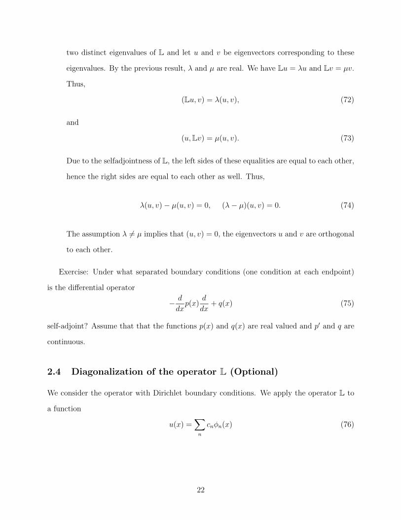
two distinct eigenvalues of L and let u and v be eigenvectors corresponding to these

eigenvalues. By the previous result, λ and µ are real. We have Lu = λu and Lv = µv.

Thus,

(Lu, v) = λ(u, v), (72)

and

(u,Lv) = µ(u, v). (73)

Due to the selfadjointness of L, the left sides of these equalities are equal to each other,

hence the right sides are equal to each other as well. Thus,

λ(u, v)− µ(u, v) = 0, (λ− µ)(u, v) = 0. (74)

The assumption λ 6= µ implies that (u, v) = 0, the eigenvectors u and v are orthogonal

to each other.

Exercise: Under what separated boundary conditions (one condition at each endpoint)

is the differential operator

− d

dxp(x)

d

dx+ q(x) (75)

self-adjoint? Assume that that the functions p(x) and q(x) are real valued and p′ and q are

continuous.

2.4 Diagonalization of the operator L (Optional)

We consider the operator with Dirichlet boundary conditions. We apply the operator L to

a function

u(x) =∑n

cnφn(x) (76)

22

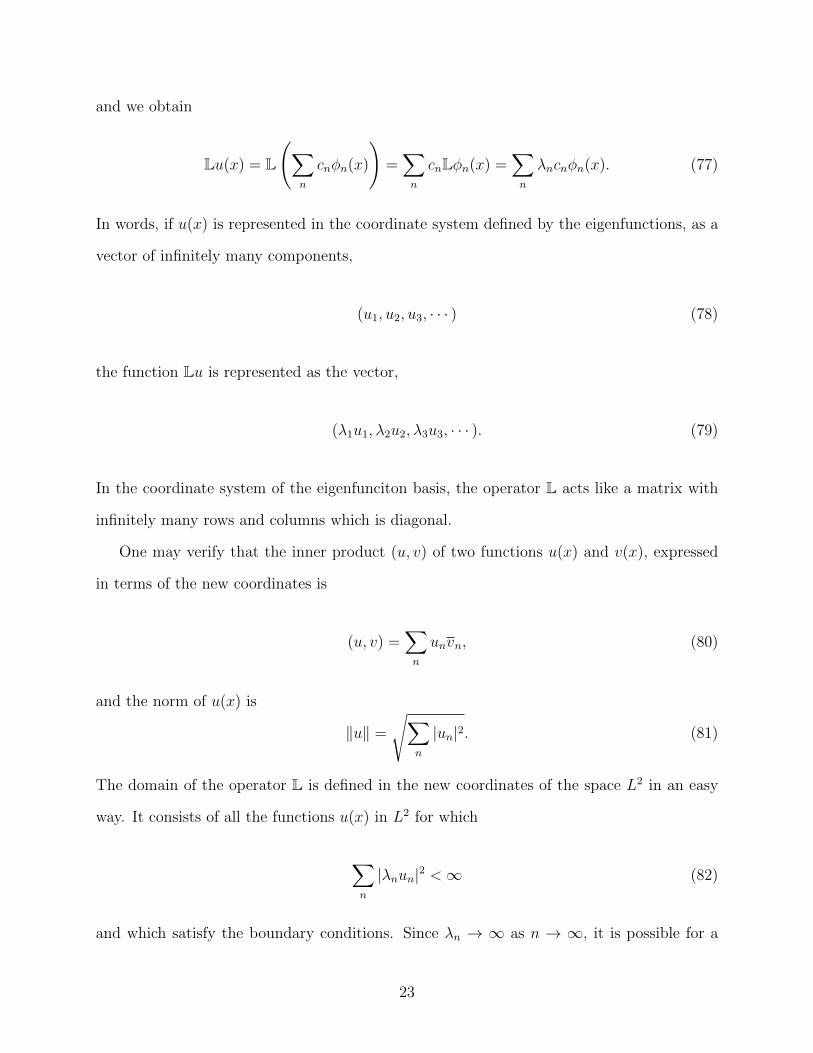
and we obtain

Lu(x) = L

(∑n

cnφn(x)

)=∑n

cnLφn(x) =∑n

λncnφn(x). (77)

In words, if u(x) is represented in the coordinate system defined by the eigenfunctions, as a

vector of infinitely many components,

(u1, u2, u3, · · · ) (78)

the function Lu is represented as the vector,

(λ1u1, λ2u2, λ3u3, · · · ). (79)

In the coordinate system of the eigenfunciton basis, the operator L acts like a matrix with

infinitely many rows and columns which is diagonal.

One may verify that the inner product (u, v) of two functions u(x) and v(x), expressed

in terms of the new coordinates is

(u, v) =∑n

unvn, (80)

and the norm of u(x) is

‖u‖ =

√∑n

|un|2. (81)

The domain of the operator L is defined in the new coordinates of the space L2 in an easy

way. It consists of all the functions u(x) in L2 for which

∑n

|λnun|2 <∞ (82)

and which satisfy the boundary conditions. Since λn → ∞ as n → ∞, it is possible for a

23

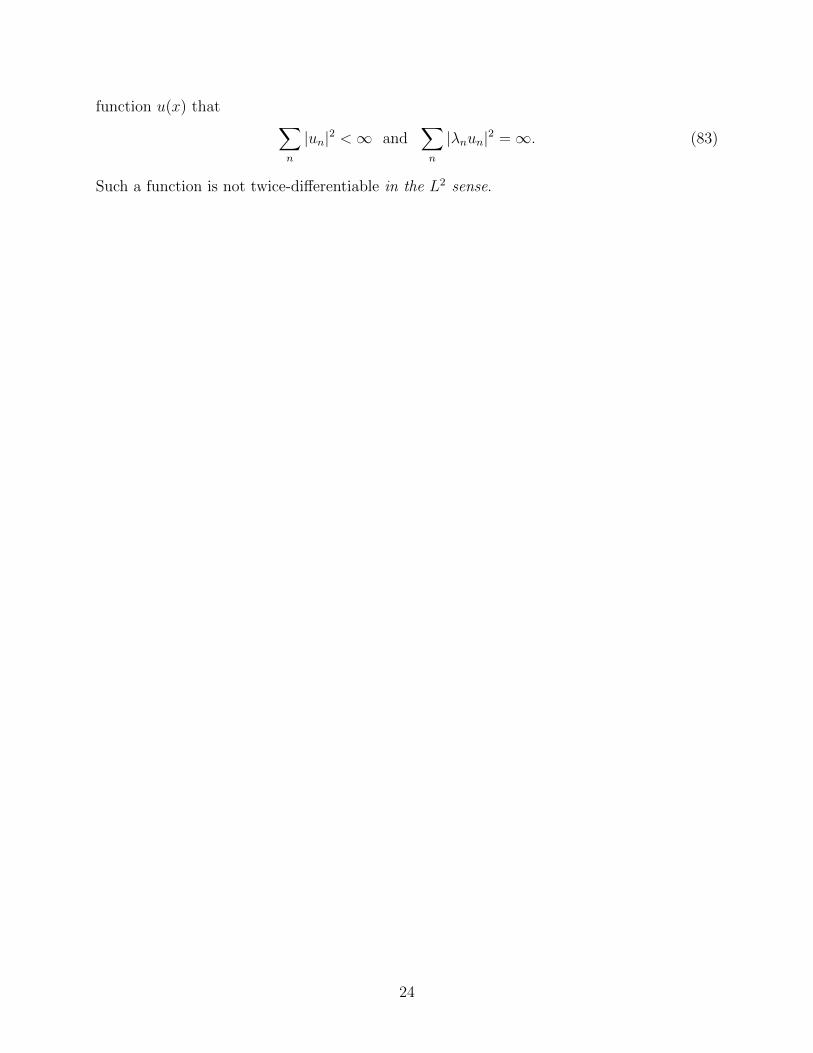
function u(x) that ∑n

|un|2 <∞ and∑n

|λnun|2 =∞. (83)

Such a function is not twice-differentiable in the L2 sense.

24

3 Derivation of the heat or diffusion equation

Henceforth we will use the shorthand notation

ut =∂u

∂t, ux =

∂u

∂x, uxx =

∂2u

∂x2. (84)

3.1 Conservation law and flux law.

A substance along the x axis has concentration (mass per unit length) u(x, t). The flux of

the material at point x (rate at which mass crosses point x from left to right) is given by

the function f(x, t). The substance cannot be created (there are no sources) and it cannot

destroyed (there are no sinks).

1. The time-rate of change of concentration at each point and time is clearly ut(x, t)

2. We now express the same rate by focusing our attention on a small interval I =

(x, x + ∆x) and considering the rates at which substance enters the interval from

either side. Assume that mass is conserved (neither created nor destroyed). and break

the calculation to the following steps.

(a) time-rate at which mass enters I at point x (known as the flux): f(x, t)

(b) time-rate at which mass exits from I at point x+ ∆x : f(x+ ∆x, t)

(c) time-rate at which nett mass enters I: f(x, t)− f(x+ ∆x, t)

(d) time-rate at which average concentration in I increases: f(x,t)−f(x+∆x,t)∆x

(e) time-rate at which concentration at point x increases: lim∆x→0f(x,t)−f(x+∆x,t)

∆x=−fx(x, t).

3. Since mass is neither created nor destroyed, the results of item 1 and item 2 are

25

necessarily equal to each other, thus:

ut + fx = 0 (85)

This equation is a conservation law. It expresses the conservation of mass.

4. The phenomenon of diffusion occurs when the substance consists of tiny particles

that make infinitesimal jumps, according to the same probability distribution for each

particle, with no preference for left or right and independently of each other. Under

these conditions, the formula for the flux is (explain why this formula is correct)

f = −Dux. (86)

where D is a positive constant.

5. Insert Eq. (86) into Eq. (85) to obtain

ut = Duxx. (87)

This is the diffusion equation.

6. If the infinitesimal jumps described show a fixed preference for left or right, a drift

occurs simulataneously with the diffusion. The equation now incorporates a drift term,

ut + cux = Duxx. (88)

where the velocity c is positive for drift to the right and negative for drift to the left.

This is the diffusion equation with drift.

7. In the presence of sources or sinks(=negative sources), a source term s(x, t) (mass per

26

unit length per unit time) must be incorporated into the equation:

ut + cux = Duxx + s(x, t). (89)

3.2 Diffusion in nature

We consider two examples from physics, assuming zero external forcing.

1. In the first example, u(x, t) is the temperature distribution along a rod, measured at

all rod points x, at time t. The rod is thermally insulated along its length, but not

at its endpoints. The quantity that justifies the derivation in this physical context

is the heat energy density Q(x, t) given by the formula Q = Ku, where u is the

temperature in degrees Kelvin and K is6 the heat cappacity per unit rod length. K

is assumed to be constant that is independent of u and also independent of x (the

rod is also assumed to be homogeneous). A higher energy density at some site x is

translated to higher mobility at the atomic and/or molecular scale. The evolution

of the energy density profile and hence of the temperature profile occurs as mobility

spreads as described above from rod regions of higher temperature to ones of lower

temperature. The conservation law (85) is the conservation of energy. The spreading

of heat energy follow the flux law (86). In this context, equation (87) is refered to as

the heat equation.

2. In the second example,

Demo http://www.youtube.com/watch?v=H7QsDs8ZRMI

u(x, t) is the profile of a low concentration of bromine gas in air, inside a thin gas-

tube. In a lab experiment, the concentration of bromine can be observed by the

intensity of its brown color. The evolution of the bromine concentration profile occurs

as bromine molecules colliding randomly with air molecules spread from higher to lower

27

concentrations according to the flux law (86). The conservation of bromine mass is

expressed by the conservation law (85).

The heat (or diffusion) equation is similarly derived in two and three spatial dimensions. In

three dimensions it is

ut = D∆u, (90)

where ∆ is the Laplace operator (or Laplacian) ∆ = ∂2

∂2x+ ∂2

∂2y+ ∂2

∂2z. As one of the many

examples of the diffusion equation is suitable for modeling in three dimensions, we mention

smoke coming out of a chimney. A drift term is added if there is wind.

28

4 PARTIAL DIFFERENTIAL EQUATIONS (PDE)

Our approach to solving linear PDE is the one outlined in the introduction of Chapter 2 of

NOTES II. In all the cases studied below, the linear operator which provides the eigenfunc-

tion basis that decouples the problem to a set of scalar ODEs is immediately identifiable and

is selfadjoint. In general, however, one seeks solutions to a linear homogeneous PDE of the

form b(t)ψ(x), that is a form of separated variables.

4.1 Separation of variables

A basic example is the heat equation

ut = Duxx (91)

for the unknown function u(x, t). The method seeks solutions of the form

u(x, t) = b(t)ψ(x), (92)

hence the name of the method. It provides particularly rich results in the case of linear

homogeneous PDE, like our example, where the solutions constructed by the method are

then linearly superposed to produce the full solution to important initial and/or boundary

value problems for those PDE. Inserting the solution form into the PDE obtains (b is the

derivative of b with respect to time),

b(t)ψ(x) = Db(t)ψ′′(x),b(t)

b(t)= D

ψ′′(x)

ψ(x)= −Dλ (93)

Necessarily, λ is a constant. Indeed, when only one of t or x is varied, neither of the two

fractions can change, because it equals the other one, that remains unchanged! We have two

29

linear ODE with constant coefficients for ψ(x) and b,

ψ′′ + λψ = 0, b = −Dλb. (94)

Solving the two ODE, we obtain the following solutions that are parametrized by λ.

u(x, t;λ) = e−Dλt cos(√λx), e−Dλt sin(

√λx). (95)

If the x variable of the PDE is restricted on an interval and if there are appropriate boundary

conditions, they will allow only a sequence of values of λ. Our approach before and the

present one are identical.

4.2 The heat equation

4.2.1 Solution of the initial-boundary value problem of the heat equation in a

bounded domain by means of eigenfunction expansions

We solve the initial value problem for the forced heat equation with zero Dirichlet boundary

conditions and an initial condition. We think of 0 < x < L as the space variable and t as

the time variable. The unknown function u(x, t) represents the temperature at the spatial

point x at time t. Alternatively, if the equation describes the diffusion of a certain substance

in the interval (0, L), then u(x, t) represents the concentration of the substance. The full

mathematical problem is

ut = Duxx + f(x, t), 0 < x < L, t > 0, (96)

• zero Dirichlet boundary conditions, u(0, t) = 0 and u(L, t) = 0,

• initial condition u(x, 0) = h(x).

30

The function f(x, t) is a source term. The coefficient D > 0 is known as the diffusion

coefficient

We rewrite the PDE as

ut = −DLu+ f(x, t), 0 < x < L, t > 0, (97)

where L is the operator − d2

dx2with zero Dirichlet boundary conditions. The method of

eigenfunction expansions, as it is commonly called, is essentially a method of undetermined

coefficients. All functions that involve the variable x are represented as a linear superposition

of the eigenfunctions of L. When these functions of space depend on time as well, the

coefficients in the series also depend on time. So,

u(x, t) = b1(t)ψ1(x) + b2(t)ψ2(x) + b3(t)ψ3(x) + · · · , (98)

The coefficients bn(t) are the unknowns of the problem. We also have the given

u(x, 0) = h(x) = h1ψ1(x) + h2ψ2(x) + h3ψ3(x) + · · · (99)

The scalar coefficients hn are calculated with the aid of formula (7). Furthermore,

f(x, t) = f1(t)ψ1(x) + f2(t)ψ2(x) + f3(t)ψ3(x) + · · · (100)

where the functions fn(t) are again calculated with the aid of formula (7).

We observe that

Lu = L{b1(t)ψ1(x) + b2(t)ψ2(x) + b3(t)ψ3(x) + · · · }

= b1(t)Lψ1(x) + b2(t)Lψ2(x) + b3L(t)ψ3(x) + · · ·

= λ1b1(t)ψ1(x) + λ2b2(t)ψ2(x) + λ3b(t)ψ3(x) + · · ·

(101)

31

We now insert the expansions for u, Lu, and f into equation (97) and balance the coefficients

of the eigenfunction ψn for each index n. We obtain a set of first order ODE for the coefficients

bn(t).

d

dtbn = −λnDbn + fn(t), n = 1, 2, 3, · · · . (102)

These are linear first order ODE, hence, solvable. The eigenvalues λn have been calculated

earlier. For each of the bn, we need the initial condition. We have already obtained this:

bn(0) = hn, n = 1, 2, 3, · · · . (103)

Everything in the right side of the solution (98) has now been calculated. The problem is

thus solved.

In the simpler, sourceless case f(x, t) ≡ 0, the solution of the ODE is immediate.

bn(t) = bn(0)eλnt. (104)

u(x, t) =∞∑n=1

hne−λnDtψn(x), where hn =

1

‖ψn‖2

∫ L

0

h(s)ψn(s)ds. (105)

We can also manipulate equations (105) further by inserting the expression for hn in the

second equation into the first equation and changing the order of summation and integration.

u(x, t) =

∫ L

0

(∞∑n=1

e−λnDtψn(x)ψn(s)

‖ψn‖2

)u(t, 0)ds (106)

The sum in the parenthesis is the function G(x, t, s) of equation (??). In this equation T

our current u and Ti is u at time zero. The sum cannot be calculated explicitly.

Inserting the eigenfunctions and eigenvalues, that correspond to zero Dirichlet boundary

conditions, into the first equation (105), one obtains the solution to the BVP

u(x, t) =∞∑n=1

hne−(nπL )

2Dt sin

nπx

L. (107)

32

The solution decays exponentially in time.

In an analogous way, one obtains the solution for Neumann boundary conditions.

u(x, t) =∞∑n=0

hne−(nπL )

2Dt cos

nπx

L. (108)

Notice that for n = 0, the cosine equals unity and the eigenvalue is zero, in agreement to

the values calculated. As t→∞, the solution converges to the constant solution

limt→∞

u(x, t) = h0 =1

L

∫ L

0

u(x, 0)dx, (109)

which is the mean value of the initial temperature distribution.

The solution is obtained in a similar way, for other boundary conditions, for which the

problem is selfadjoint.

Nonhomogeneous boundary conditions: We let u(x, t) = v(x, t) + a(x, t) where

a(x, t) is some function that satisfies the boundary conditions required of u(x, t). As a result

v(x, t) satisfies zero boundary conditions. Inserting the expression for u into the PDE we

obtain a heat equation, for v. The function a appears in the forcing term.

4.3 The wave equation

4.3.1 Derivation

The standard textbook example is the vibrating string with small amplitude oscillations.

This is a transverse wave. It propagates along the string, while oscillation occurs transver-

sly to the string. We derive the wave equation in the context of a longitudinal wave, i.e.

one in which the oscillation occurs along the direction of propagation. We obtain the wave

equation as a limiting case of the equations of isentropic gas dynamics in one space dimen-

sion, which we derive first. The variables in the equations of gas dynamics are the gas density

ρ(x, t) and the velocity u(x, t) of the of the gas particles at the position x and time t. The

33

wave propagates in the x direction, while all its characteristics remain constant along the

planes that are perpendicular to the x direction. Conservation of mass:

(concentration: gas density ρ; flux: ρu).

ρt + (ρu)x = 0 (110)

Momentum equation (conservation law with source):

(concentration: momentum density ρu; flux: ρu2; pressure: p, taken to be an

increasing function of ρ)

(ρu)t + (ρu2)x = −p(ρ)x (111)

Utilizing the first equation, we can simplify the second one to

ρut + ρuux + p′(ρ)ρx = 0 (112)

The system of the two equations (110) and (112) for the density ρ(x, t) and the veloc-

ity u(x, t) constitute the equations of isentropic gas dynamics. The system is clearly

nonlinear.

We now assume that the velocity u of the gas particles is very small and that the difference

of the density ρ from a constant value ρ0 is also very small. We make no smallness assumption

for the space and time derivatives of the velocity u and the density ρ. This is the acoustic limit

of the equations of gas dynamics (u is not the speed of sound). The smallness assumption

on u allows us to neglect terms of the equations that are in the small scale compared to

the other terms. These are (1) the term uρx that arises in Eq. (110) after one applies the

product rule and (2) the middle term ρuux of Eq. (112). The smallness in the deviation

of ρ from ρ0 allows us to replace ρ by ρ0 when no derivative of ρ is taken. The system of

34

equations of gas dynamics becomes in this limit

ρt + ρoux = 0,

ρ0ut + p′(ρ0)ρx = 0.

(113)

This is a linear system.

Taking the derivative with respect to t in the first equation and the derivative with respect

to x in the second equation, and eliminating the term uxt that appears in both equations,

we obtain,

ρtt − p′(ρ)ρxx = 0 (114)

This is the wave equation. Notice that by taking the derivative of the first equation with

respect to x and the second one with threspect to t,and eliminating the term ρxt, we obtain

utt − p′(ρ)uxx = 0 (115)

The density ρ and the particle velocity u satisfy the same wave equation. As we see below,

the significance of p′(ρ) is that the sound-speed is√p′(ρ).

4.3.2 General solution on the line and the d’Alambert solution formula

As the name “wave” impies, the solutions of the wave equation are oscillatory. Thus, the

wave equation describes fundamentally different physical behaviors from those of the heat

(or diffusion) equation, which works by tending to minimize gradients.

The wave equation in one space dimension is

utt − c2uxx = 0. (116)

35

One readily verifies that the PDE is satisfied by the expression

u(x, t) = F (x− ct) +G(x+ ct), (117)

where F and G are arbitrary functions. Moreover, the above expression gives the general

solution of the wave equation on the real spatial line.The left term represents a wave traveling

to the right at speed c (we assume c > 0), while the right term represents a wave traveling

to the left at speed c. As the wave equation is of second order in time, we need two initial

conditions, u(x, 0) and ut(x, 0). Given

u(x, 0) = f(x), ut(x, 0) = g(x), (118)

we can calculate the functions F and G. Indeed,

F (x) +G(x) = f(x), −cF ′(x) + cG′(x) = g(x). (119)

Taking the derivative of the first equation, leaves us with a system of two equations for the

two unknowns F ′(x) and G′(x). We find

F ′(x) =1

2f ′(x)− 1

2cg(x), G′(x) =

1

2f ′(x) +

1

2cg(x). (120)

We integrate these

F (x) =1

2f(x)− 1

2ch(x), G(x) =

1

2f(x) +

1

2ch(x), (121)

where (a) h(x) is any antiderivative of g(x) and (b) the antiderivative of f ′ has been chosen

to be f , so that the first of equations (119) is satisfied. Inserting these into equation (117),

36

we obtain

u(x, t) =1

2f(x− ct)− 1

2ch(x) +

1

2f(x+ ct) +

1

2ch(x+ ct)

1

2{f(x− ct) + f(x+ ct)}+

1

2c{h(x+ ct)− h(x− ct)}.

(122)

Recalling that h is an antiderivative of g, we derive the D’Alambert formula for the solution,

u(x, t) =1

2{f(x− ct) + f(x+ ct)}+

1

2c

∫ x+ct

x−ctg(s)ds}. (123)

Notice that if g ≡ 0, the signal f(x) breaks up into two identical pieces, that travel in

opposite directions at speed c. It is also instructive to examine the solution when f ≡ 0 and

g is a delta function centered at x = 0.

The wave equation in higher dimensions is

utt − c2∆u = 0, (124)

where ∆u = uxx + uyy in two spatial variables and ∆u = uxx + uyy + uzz in three spatial

variables.

4.3.3 Solution of the initial-boundary value problem for the wave equation in

a bounded domain by means of eigenfunction expansions

In spite of the behavioral differences, between the wave and heat equations, the procedure for

solving the IBVP is the same. So we only outline the procedure. Nevertheless, the neophyte

can only master it but filling in all the details.

We first write the equation as

utt + c2Lu = 0. (125)

We let

u(x, t) = b1(t)ψ1(x) + b2(t)ψ2(x) + b3(t)ψ3(x) + · · · , (126)

37

As with the heat equation, we obtain an infinite number of uncoupled ODE for the bn:

d2

dt2bn + c2λnbn = 0. (127)

The general solution of the equation for bn is

bn = An cos(c√λnt) +Bn sin(c

√λnt). (128)

The time evolution of each of the solution modes is oscillatory, in stark contrast to the

behavior of the heat equation. The constants An and Bn are obtained from our knowledge

of bn(0) and bn(0) (a dot indicates a time derivative).

4.4 The Laplace equation: A boundary value problem (BVP)

4.4.1 Derivation and significance

Laplace’s equation in three spatial dimensions is

∆u = uxx + uyy + uzz = 0. (129)

When it includes a non-homogeneous term,

uxx + uyy + uzz = −ρ(x, y, z), (130)

it is referred to as the Poisson equation. The Laplacian operator

∆ =∂2

∂2x+

∂2

∂2y+

∂2

∂2z, (131)

38

is the divergence of the gradient,

∆u = ∇ · ∇u = div gradu, (132)

a fact that gives it great significance in physics. Indeed, some important force fields in

physics, including the elctrostatic field and the Newtonian gravitational fileld, are represented

as the negative gradient of a scalar field u(x, y, z), called the potential. Fields arising from

a potential in this way are called potential fields. Denoting such a field by F(x, y, z), we

have

F(x, y, z) = −∇u. (133)

Then, by Eq. (132)

∆u = −∇ · F(x, y, z). (134)

The divergence of a force field is a scalar field that can, in turn, be understood as the source

density of the force field. For example, mass density is the source density for the Newtonian

gravitational field and electric charge density for the electrostatic field. In general the term

ρ(x, y, z)in the Poisson equation, is the source density of the field generated by the potential

u(x, y, z). It happens often that all field sources lie outside the spatial region of interest.

The potential then satisfies Laplace’s equation (129) in this region.

The precise connection between a potential field and its source-density is provided by the

divergence theorem which states that the outward flux of the field across the boundary of a

bounded region in space (this is a double integral) equals the triple integral over this region

of the source density. In the limit of the region being a sphere of very small radius, centerd

at some point x the connection becomes obvious.

39

4.4.2 Solution of the boundary value problem for the Laplace equation by means

of eigenfunction expansions

The Laplace and Poisson equations are often posed on a bounded domain, for example

inside of a sphere, with a boundary condition all around the boundary. We solve the Laplace

equation in two space dimensions on a semi-infinite strip. We let

∆u = uxx + uyy = 0, (135)

inside the semi-infinite strip of the x, y plane defined by 0 < x < L and y > 0. We impose one

boundary condition along the half-line x = 0, y > 0 and one along the half-line x = L, y > 0.

In order to be able to apply directly the techniques that we have developed, we require these

boundary conditions to be homogeneous. We also impose a boundary condition, generally

non-homogeneous, on the interval 0 < x < L on the real axis. Finally, we require that the

solution to the Laplace equation be bounded in the strip, that is it must remain smaller in

absolute value than some finite value. This prohibits the solution to grow without bound as

y → +∞; thus, it is essentially a boundary condition at y = +∞.

As in the case of the heat equation, we write te PDE as

uyy − Lu = 0, L = − d2

dx2, (136)

Example 1: Dirichlet boundary conditions. We choose zero Dirichlet boundary condi-

tions at x = 0 and x = L, that is u(0, y) = 0 and u(L, y) = 0. We also choose the Dirichlet

condition

u(x, 0) = h(x) = b1(0)ψ1(x) + b2(0)ψ2(x) + b3(0)ψ3(x) + · · · , ψn(x) = sinnπx

L, (137)

on the interval (0, L) on the x axis, where ψn(x) is the eigenfunction corresponding to the

eigenvalue λn of the operator L. The coefficients hn are calculated as usual from formula

40

(7). We let

u(x, y) = b1(y)ψ1(x) + b2(y)ψ2(x) + b3(y)ψ3(x) + · · · , (138)

and insert it into (136). By the usual procedure, we obtain the following ODE for the bns.

d2bndy2− λnbn = 0, λn =

(nπL

)2

, n = 1, 2, 3, · · · , (139)

with solution basis

e−√λny and e

√λny. (140)

The solution e√λny violates the boundedness condition as y → +∞ and is rejected. Thus,

u(x, y) = b1(0)e−πyL sin

πx

L+ b2(0)e−

2πyL sin

2πx

L+ · · ·+ bn(0)e−

nπyL sin

nπx

+· · · (141)

The solution tends to zero exponentially, as y → +∞.

Example 2: Neumann conditions and the existence of a nullspace. We change the

boundary conditions from Dirichlet to Neumann. So ux(0, y) = 0, ux(L, y) = 0 on the two

half-lines of the boundary and uy(x, 0) = h(x) on the interval. In order to avoid jumps of

the boundary condition, we require h(0) = h(x) = 0. The proper basis to use in representing

the solution, is the eigenvectors of the operator L with Neumann conditions (see (57))

1, cosπx

L, cos

2πx

L· · · , cos

nπx

L, · · · , (142)

with eigenvalues

0,(πxL

)2

,

(2πx

L

)2

, · · ·(nπxL

)2

, · · · , (143)

respectively. So,

u(x, y) = b0(y) + b1(y) cosπx

L+ b2(y) cos

2πx

L+ · · ·+ bn(y) cos

nπx

L+ · · · (144)

41

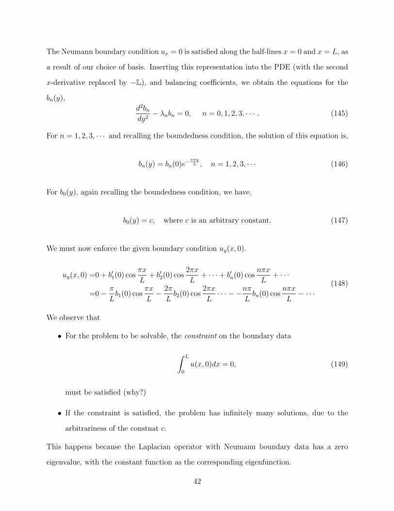
The Neumann boundary condition ux = 0 is satisfied along the half-lines x = 0 and x = L, as

a result of our choice of basis. Inserting this representation into the PDE (with the second

x-derivative replaced by −L), and balancing coefficients, we obtain the equations for the

bn(y),

d2bndy2− λnbn = 0, n = 0, 1, 2, 3, · · · . (145)

For n = 1, 2, 3, · · · and recalling the boundedness condition, the solution of this equation is,

bn(y) = bn(0)e−nπyL , n = 1, 2, 3, · · · (146)

For b0(y), again recalling the boundedness condition, we have,

b0(y) = c, where c is an arbitrary constant. (147)

We must now enforce the given boundary condition uy(x, 0).

uy(x, 0) =0 + b′1(0) cosπx

L+ b′2(0) cos

2πx

L+ · · ·+ b′n(0) cos

nπx

L+ · · ·

=0− π

Lb1(0) cos

πx

L− 2π

Lb2(0) cos

2πx

L· · · − −nπ

Lbn(0) cos

nπx

L− · · ·

(148)

We observe that

• For the problem to be solvable, the constraint on the boundary data

∫ L

0

u(x, 0)dx = 0, (149)

must be satisfied (why?)

• If the constraint is satisfied, the problem has infinitely many solutions, due to the

arbitrariness of the constnat c.

This happens because the Laplacian operator with Neumann boundary data has a zero

eigenvalue, with the constant function as the corresponding eigenfunction.

42

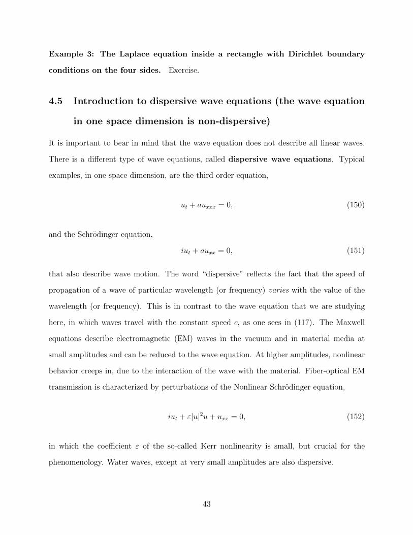
Example 3: The Laplace equation inside a rectangle with Dirichlet boundary

conditions on the four sides. Exercise.

4.5 Introduction to dispersive wave equations (the wave equation

in one space dimension is non-dispersive)

It is important to bear in mind that the wave equation does not describe all linear waves.

There is a different type of wave equations, called dispersive wave equations. Typical

examples, in one space dimension, are the third order equation,

ut + auxxx = 0, (150)

and the Schrodinger equation,

iut + auxx = 0, (151)

that also describe wave motion. The word “dispersive” reflects the fact that the speed of

propagation of a wave of particular wavelength (or frequency) varies with the value of the

wavelength (or frequency). This is in contrast to the wave equation that we are studying

here, in which waves travel with the constant speed c, as one sees in (117). The Maxwell

equations describe electromagnetic (EM) waves in the vacuum and in material media at

small amplitudes and can be reduced to the wave equation. At higher amplitudes, nonlinear

behavior creeps in, due to the interaction of the wave with the material. Fiber-optical EM

transmission is characterized by perturbations of the Nonlinear Schrodinger equation,

iut + ε|u|2u+ uxx = 0, (152)

in which the coefficient ε of the so-called Kerr nonlinearity is small, but crucial for the

phenomenology. Water waves, except at very small amplitudes are also dispersive.

43

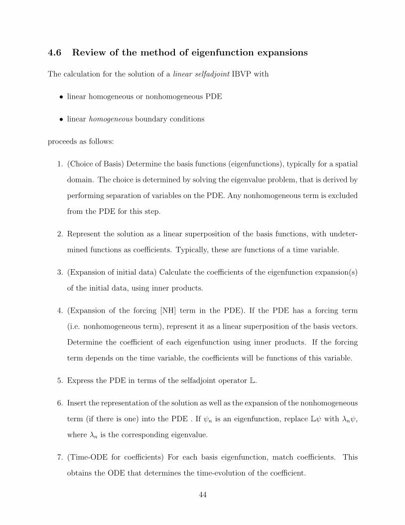
4.6 Review of the method of eigenfunction expansions

The calculation for the solution of a linear selfadjoint IBVP with

• linear homogeneous or nonhomogeneous PDE

• linear homogeneous boundary conditions

proceeds as follows:

1. (Choice of Basis) Determine the basis functions (eigenfunctions), typically for a spatial

domain. The choice is determined by solving the eigenvalue problem, that is derived by

performing separation of variables on the PDE. Any nonhomogeneous term is excluded

from the PDE for this step.

2. Represent the solution as a linear superposition of the basis functions, with undeter-

mined functions as coefficients. Typically, these are functions of a time variable.

3. (Expansion of initial data) Calculate the coefficients of the eigenfunction expansion(s)

of the initial data, using inner products.

4. (Expansion of the forcing [NH] term in the PDE). If the PDE has a forcing term

(i.e. nonhomogeneous term), represent it as a linear superposition of the basis vectors.

Determine the coefficient of each eigenfunction using inner products. If the forcing

term depends on the time variable, the coefficients will be functions of this variable.

5. Express the PDE in terms of the selfadjoint operator L.

6. Insert the representation of the solution as well as the expansion of the nonhomogeneous

term (if there is one) into the PDE . If ψn is an eigenfunction, replace Lψ with λnψ,

where λn is the corresponding eigenvalue.

7. (Time-ODE for coefficients) For each basis eigenfunction, match coefficients. This

obtains the ODE that determines the time-evolution of the coefficient.

44

8. (Solve ODE) Solve the ODE that determine the time-evolution of these coefficients.

The results of the item (3) provide the initial data for the ODE in question.

9. (Superposition of contributions) Sum the contributions from all eigenfunctions to derive

the solution of the IBVP.

Important remarks

1. The eigenvalue problem referred to in item (1) above, that makes the choice of the

basis, is obtained by applying the separation of variables to the PDE from which the

forcing term (if there is one) is omitted. By separation of variables is meant seeking a

solution of the homogeneous PDE of the form b(t)ψ(x).

2. If the operator (including the boundary conditions) one obtains in this way is selfad-

joint, it is guaranteed by theorem that

(a) the eigenvalues are real

(b) the eigenfunctions are mutually orthogonal and form a complete set, thus they

can be used as a basis.

3. One may refer to the eigenfunctions ψn(x) as the spatial modes of which the solution

is made up at each time t. The coefficients b(t) describe the “amplitude” with which

each mode participates in the solution at time t. A basis function participates in the

solution (its coefficient is not identically zero) if

(a) its coefficient in the expansion of the initial data is nonzero or

(b) its coefficient in the series for the forcing term is not identically zero.

4. Most important: Each mode evolves independently of any other mode. So for example,

if only one mode has a nonzero coefficient in the initial data and if only this mode and

two others appear in the expansion of the forcing term, the solution will only involve

three eigenfunctions. The evolution of the modes is not coupled. The decoupling has

been achieved through the eigenfunction expansion.

45

4.7 The Fourier transform

We consider the eigenvalue problem for the operator L = − d2

dx2on the whole real x line,

acting on twice differentiable L(−∞,+∞) functions,

Lψ = λψ. (153)

We obtain,

“eigenfunctions” : eikx, “eigenvalues” : λ = k2, k ∈ R. (154)

When k has a nonzero imaginary part, the function eikx displays exponential growth and

is inadmissible. Even with the admitted real values of k, the “eigenfunctions” eikx are not

in the space L(−∞,+∞). Nevertheless, we want to use the “eigenfunctions” eikx as an

improper kind of basis of L(−∞,+∞). We are forced to take linear superpositions of the

basis functions using integration instead of summation. This reflects the fact that k is not

a discrete parameter, but takes values over a continuum. We want to represent a function

f(x) in L(−∞,+∞) as

f(x) =1

2π

∫ ∞−∞

f(k)eikxdk, (155)

where f(k)2π

plays the role of the coefficient in our earlier series representations and k is a

continuous analogue of the index of summation in series eigenfunction expansions.

As we did with proper eigenfunctions, we will establish an “orthogonality” relation be-

tween eikx and eilx when k 6= l, ignoring momentarily that the functions involved are not in

L2. To prove is the relation

(eikx, eilx) =

∫ ∞−∞

eikxeilxdx = 2πδ(k − l), (156)

where δ is the Dirac delta function. Recalling that the complex conjugate of eilx is e−ilx and

46

letting k − l = a, we can rewrite this relation as

∫ ∞−∞

eiaxdx = 2πδ(a). (157)

The integral on the left is not a classical improper integral. If we integrate it in a large

interval [−N,+N ], we find the value 2 sin(aN)a

. This oscillates as N → ∞, there is no limit.

For such oscillatory integrals, instead of the sharp cut-off at ±N , we make a smooth cut-off

by multiplying the integrand by the factor e−εx2. When ε > 0 is small, the effect of the factor

is felt only at high values of x providing superexponential decay as x→∞. As the smooth

cut-off is removed in the limit ε→ 0, we obtain the right hand side of equation (157). The

following string of equations illustrates the procedure. The calculation of then integral and

its limit follow.

∫ ∞−∞

eiaxdx = limε↘0

∫ ∞−∞

eiax−εx2

dx = 2π limε↘0

(e−

a2

4ε

√4πε

)= 2πδ(a). (158)

Proof of (158).

• Calculation of the integral: We prove the above limit by, first, calculating the integral,

J(a) =

∫ ∞−∞

eiax−εx2

dx. (159)

We take the derivative with respect to a and integrate by parts,

dJ

da= i

∫ ∞−∞

xeiaxe−εx2

dx = − i

2ε

∫ ∞−∞

eiaxde−εx2

= − a

2ε

∫ ∞−∞

eiax−εx2

dx = −aJ2ε.

(160)

The ODE obtained,

dJ

da= −aJ

2ε, (161)

47

is separable and is solved easily,

J(a) = J(0)e−a2

4ε , J(0) =

∫ ∞−∞

e−εx2

dx. (162)

There is a famous trick for evaluating the important integral J(0) (it is the gaussian):

calculate J(0)2 and use polar coordinates.

J(0)2 =

(∫ ∞−∞

e−εx2

dx

)(∫ ∞−∞

e−εy2

dy

)=

∫ ∞−∞

∫ ∞−∞

e−ε(x2+y2)dxdy

= 2π

∫ ∞0

e−εr2

rdr =π

ε.

(163)

Thus,

J(0) =

∫ ∞−∞

e−εx2

dx =

√π

ε. (164)

• The limit ε ↘ 0: The quantity in parenthesis in (158) is the normal probability

distribution; its graph is the well-known bell-shaped gaussian curve. The area under

the graph equals 1 (calculation identical to integral of Eq. (164) above). As ε ↘ 0,

the distribution becomes tall, with its mass concentrated closer and closer to a = 0.

It, thus, tends to the Dirac delta function.

This completes the proof of relation (157).

We now apply orthogonality to calculate f(k) in the representation (155).

f(x) =1

2π

∫ ∞−∞

f(l)eilxdl (165)

(f(x), eikx) =1

2π

(∫ ∞−∞

f(l)eilxdl, eikx)

(166)

The next step involves a change in the order of integration.

(f(x), eikx) =1

2π

∫ ∞−∞

f(l)(eilx, eikx)dl (167)

48

We use the orthogonality relation (156)

(f(x), eikx) =

∫ ∞−∞

f(l)δ(l − k)dl (168)

∫ ∞−∞

f(x)e−ilx = f(l), (169)

The pair of relations

f(k) =

∫ ∞−∞

f(x)e−ilx, f(x) =1

2π

∫ ∞−∞

f(k)eikxdlk (170)

are known as the Fourier Transform and the Inverse Fourier Transform, respectively.

Some important properties of the Fourier transform (FT).

• FT is a linear transformation

• FT: ddx

to ik.

• Convolution f ∗ g =∫∞−∞ f(x− y)g(y)dy to f(k)g(k)

• for f and g in L2, (f, g) = 12π

(f , g)

• for f in L2, ‖f‖2 = 12π‖f‖2 (equal energy in space and in frequency)

4.8 PDE applications of Fourier Transform

4.8.1 The initial value problem for the Schrodinger Equation on the line

Solve the initial value problem (IVP)

iut + uxx = 0, x ∈ R, t > 0, (171)

with initial condition

u(x, 0) = f(x). (172)

49

Solution: Take the Fourier transform of the PDE

iut + uxx = 0 (173)

iut + (ik)2u = 0, ut + ik2u = 0, (174)

u(k, t) = c(k)e−ik2t (175)

Determine the constant c(k) using the initial condition: u(k, 0) = c(k), thus, c(k) = f(k).

The Fourier transform of the solution of the IVP is ,

u(k, t) = f(k)e−ik2t (176)

Apply the inverse Fourier transform in order to obtain the solution.

u(x, t) =1

2π

∫ ∞−∞

f(k)eikx−ik2tdk. (177)

50