Section 5.5

Complex Eigenvalues

A Matrix with No Eigenvectors

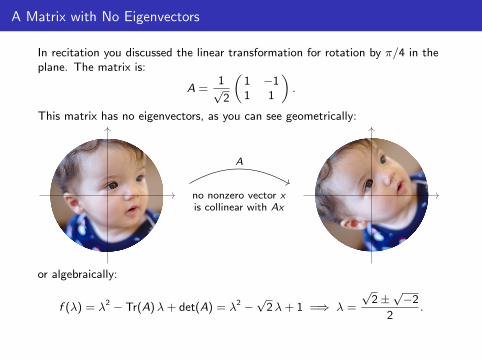
In recitation you discussed the linear transformation for rotation by π/4 in theplane. The matrix is:

A =1√2

(1 −11 1

).

This matrix has no eigenvectors, as you can see geometrically:

A

no nonzero vector xis collinear with Ax

or algebraically:

f (λ) = λ2 − Tr(A)λ+ det(A) = λ2 −√

2λ+ 1 =⇒ λ =

√2±√−2

2.

Complex Numbers

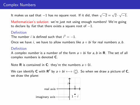
It makes us sad that −1 has no square root. If it did, then√−2 =

√2 ·√−1.

Mathematician’s solution: we’re just not using enough numbers! We’re goingto declare by fiat that there exists a square root of −1.

DefinitionThe number i is defined such that i2 = −1.

Once we have i , we have to allow numbers like a + bi for real numbers a, b.

DefinitionA complex number is a number of the form a + bi for a, b in R. The set of allcomplex numbers is denoted C.

Note R is contained in C: they’re the numbers a + 0i .

We can identify C with R2 by a + bi ←→(ab

). So when we draw a picture of C,

we draw the plane:

real axis

imaginary axis

1i

1− i

Why This Is Not A Weird Thing To DoAn anachronistic historical aside

In the beginning, people only used counting numbers for, well, counting things:1, 2, 3, 4, 5, . . .. Then someone (Persian mathematician Muh. ammad ibn Musaal-Khwarizmı, 825) had the ridiculous idea that there should be a number 0 thatrepresents an absence of quantity. This blew everyone’s mind.

Then it occurred to someone (Chinese mathematician Liu Hui, c. 3rd century) thatthere should be negative numbers to represent a deficit in quantity. That seemedreasonable, until people realized that 10 + (−3) would have to equal 7. This is whenpeople started saying, “bah, math is just too hard for me.”

At this point it was inconvenient that you couldn’t divide 2 by 3. Thus someone(Indian mathematician Aryabhatta, c. 5th century) invented fractions (rationalnumbers) to represent fractional quantities. These proved very popular. ThePythagoreans developed a whole belief system around the notion that any quantityworth considering could be broken down into whole numbers in this way.

Then the Pythagoreans (c. 6th century BCE) discovered that the hypotenuse of an

isosceles right triangle with side length 1 (i.e.√

2) is not a fraction. This caused aserious existential crisis and led to at least one death by drowning. The real number√

2 was thus invented to solve the equation x2 − 2 = 0.

So what’s so strange about inventing a number i to solve the equation x2 + 1 = 0?

Operations on Complex Numbers

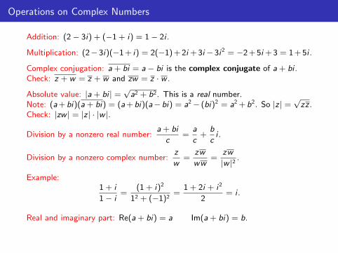
Addition: (2− 3i) + (−1 + i) = 1− 2i .

Multiplication: (2−3i)(−1 + i) = 2(−1) + 2i + 3i −3i2 = −2 + 5i + 3 = 1 + 5i .

Complex conjugation: a + bi = a− bi is the complex conjugate of a + bi .Check: z + w = z + w and zw = z · w .

Absolute value: |a + bi | =√a2 + b2. This is a real number.

Note: (a+bi)(a + bi) = (a+bi)(a−bi) = a2− (bi)2 = a2 +b2. So |z | =√zz .

Check: |zw | = |z | · |w |.

Division by a nonzero real number:a + bi

c=

a

c+

b

ci .

Division by a nonzero complex number:z

w=

zw

ww=

zw

|w |2 .

Example:1 + i

1− i=

(1 + i)2

12 + (−1)2=

1 + 2i + i2

2= i .

Real and imaginary part: Re(a + bi) = a Im(a + bi) = b.

Polar Coordinates for Complex Numbers

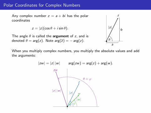
Any complex number z = a + bi has the polarcoordinates

z = |z |(cos θ + i sin θ).

The angle θ is called the argument of z , and isdenoted θ = arg(z). Note arg(z) = − arg(z).

|z|

z

a

b

θ

When you multiply complex numbers, you multiply the absolute values and addthe arguments:

|zw | = |z | |w | arg(zw) = arg(z) + arg(w).

|z|

z

|w |

w

θϕ

|z| |w |

zw

θ + ϕ

Poll

Does every square matrix have an eigenvalue, if we include complexeigenvalues?

Yes. Every polynomial can be factored completely if we include complexnumbers, so the characteristic polynomial will have at least one root!

The Fundamental Theorem of Algebra

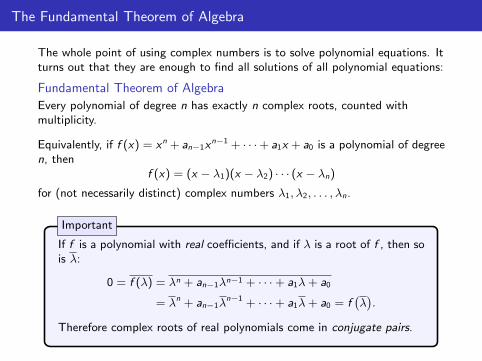
The whole point of using complex numbers is to solve polynomial equations. Itturns out that they are enough to find all solutions of all polynomial equations:

Fundamental Theorem of Algebra

Every polynomial of degree n has exactly n complex roots, counted withmultiplicity.

Equivalently, if f (x) = xn + an−1xn−1 + · · ·+ a1x + a0 is a polynomial of degree

n, thenf (x) = (x − λ1)(x − λ2) · · · (x − λn)

for (not necessarily distinct) complex numbers λ1, λ2, . . . , λn.

If f is a polynomial with real coefficients, and if λ is a root of f , then sois λ:

0 = f (λ) = λn + an−1λn−1 + · · ·+ a1λ+ a0

= λn + an−1λn−1 + · · ·+ a1λ+ a0 = f

(λ).

Therefore complex roots of real polynomials come in conjugate pairs.

Important

The Fundamental Theorem of AlgebraExamples

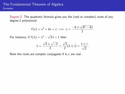
Degree 2: The quadratic formula gives you the (real or complex) roots of anydegree-2 polynomial:

f (x) = x2 + bx + c =⇒ x =−b ±

√b2 − 4c

2.

For instance, if f (λ) = λ2 −√

2λ+ 1 then

λ =

√2±√−2

2=

√2

2(1± i) =

1± i√2.

Note the roots are complex conjugates if b, c are real.

The Fundamental Theorem of AlgebraExamples

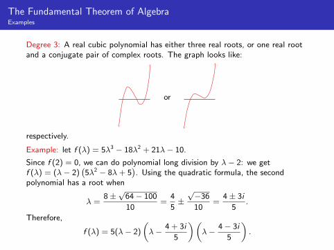
Degree 3: A real cubic polynomial has either three real roots, or one real rootand a conjugate pair of complex roots. The graph looks like:

or

respectively.

Example: let f (λ) = 5λ3 − 18λ2 + 21λ− 10.

Since f (2) = 0, we can do polynomial long division by λ− 2: we getf (λ) = (λ− 2)

(5λ2 − 8λ+ 5

). Using the quadratic formula, the second

polynomial has a root when

λ =8±√

64− 100

10=

4

5±√−36

10=

4± 3i

5.

Therefore,

f (λ) = 5(λ− 2)

(λ− 4 + 3i

5

)(λ− 4− 3i

5

).

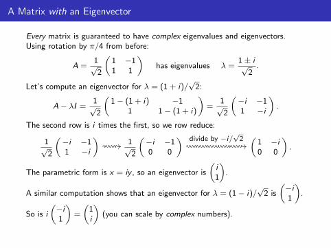
A Matrix with an Eigenvector

Every matrix is guaranteed to have complex eigenvalues and eigenvectors.Using rotation by π/4 from before:

A =1√2

(1 −11 1

)has eigenvalues λ =

1± i√2.

Let’s compute an eigenvector for λ = (1 + i)/√

2:

A− λI =1√2

(1− (1 + i) −1

1 1− (1 + i)

)=

1√2

(−i −11 −i

).

The second row is i times the first, so we row reduce:

1√2

(−i −11 −i

)1√2

(−i −10 0

) divide by −i/√

2 (1 −i0 0

).

The parametric form is x = iy , so an eigenvector is

(i1

).

A similar computation shows that an eigenvector for λ = (1− i)/√

2 is

(−i1

).

So is i

(−i1

)=

(1i

)(you can scale by complex numbers).

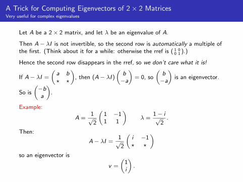
A Trick for Computing Eigenvectors of 2 × 2 MatricesVery useful for complex eigenvalues

Let A be a 2× 2 matrix, and let λ be an eigenvalue of A.

Then A− λI is not invertible, so the second row is automatically a multiple ofthe first. (Think about it for a while: otherwise the rref is ( 1 0

0 1 ).)

Hence the second row disappears in the rref, so we don’t care what it is!

If A− λI =

(a b? ?

), then (A− λI )

(b−a

)= 0, so

(b−a

)is an eigenvector.

So is

(−ba

).

Example:

A =1√2

(1 −11 1

)λ =

1− i√2.

Then:

A− λI =1√2

(i −1? ?

)so an eigenvector is

v =

(1i

).

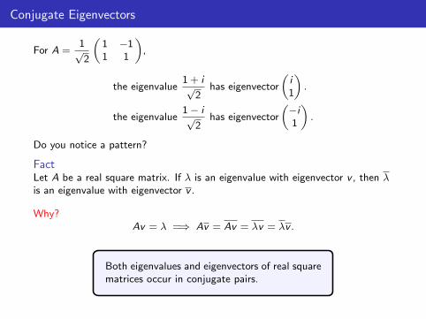
Conjugate Eigenvectors

For A =1√2

(1 −11 1

),

the eigenvalue1 + i√

2has eigenvector

(i1

).

the eigenvalue1− i√

2has eigenvector

(−i1

).

Do you notice a pattern?

FactLet A be a real square matrix. If λ is an eigenvalue with eigenvector v , then λis an eigenvalue with eigenvector v .

Why?Av = λ =⇒ Av = Av = λv = λv .

Both eigenvalues and eigenvectors of real squarematrices occur in conjugate pairs.

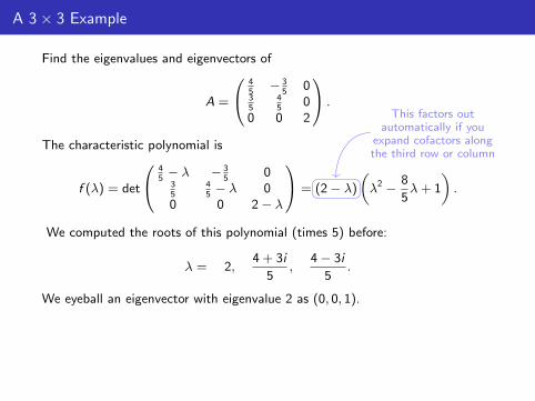
A 3 × 3 Example

Find the eigenvalues and eigenvectors of

A =

45− 3

50

35

45

00 0 2

.

The characteristic polynomial is

f (λ) = det

45− λ − 3

50

35

45− λ 0

0 0 2− λ

= (2− λ)

(λ2 − 8

5λ+ 1

).

This factors outautomatically if you

expand cofactors alongthe third row or column

We computed the roots of this polynomial (times 5) before:

λ = 2,4 + 3i

5,

4− 3i

5.

We eyeball an eigenvector with eigenvalue 2 as (0, 0, 1).

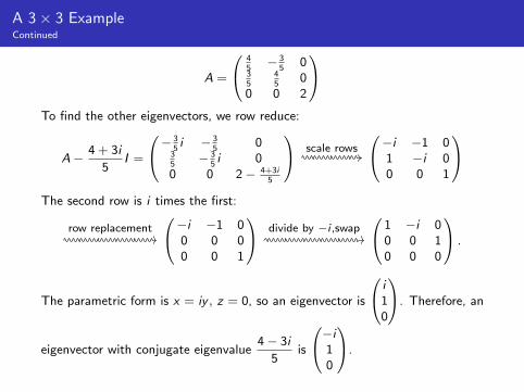
A 3 × 3 ExampleContinued

A =

45− 3

50

35

45

00 0 2

To find the other eigenvectors, we row reduce:

A− 4 + 3i

5I =

− 35i − 3

50

35

− 35i 0

0 0 2− 4+3i5

scale rows

−i −1 01 −i 00 0 1

The second row is i times the first:

row replacement−i −1 0

0 0 00 0 1

divide by −i ,swap 1 −i 0

0 0 10 0 0

.

The parametric form is x = iy , z = 0, so an eigenvector is

i10

. Therefore, an

eigenvector with conjugate eigenvalue4− 3i

5is

−i10

.

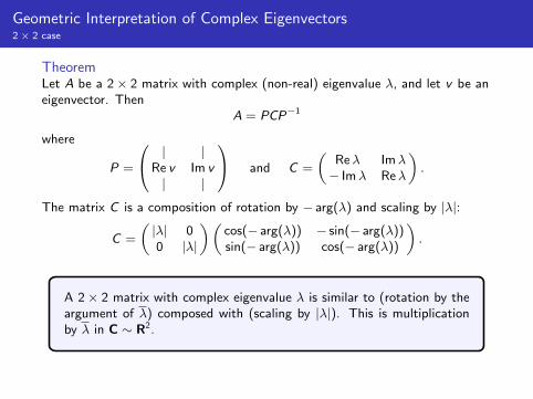
Geometric Interpretation of Complex Eigenvectors2 × 2 case

TheoremLet A be a 2× 2 matrix with complex (non-real) eigenvalue λ, and let v be aneigenvector. Then

A = PCP−1

where

P =

| |Re v Im v| |

and C =

(Reλ Imλ− Imλ Reλ

).

The matrix C is a composition of rotation by − arg(λ) and scaling by |λ|:

C =

(|λ| 00 |λ|

)(cos(− arg(λ)) − sin(− arg(λ))sin(− arg(λ)) cos(− arg(λ))

).

A 2× 2 matrix with complex eigenvalue λ is similar to (rotation by theargument of λ) composed with (scaling by |λ|). This is multiplicationby λ in C ∼ R2.

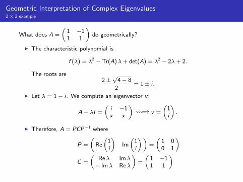
Geometric Interpretation of Complex Eigenvalues2 × 2 example

What does A =

(1 −11 1

)do geometrically?

I The characteristic polynomial is

f (λ) = λ2 − Tr(A)λ+ det(A) = λ2 − 2λ+ 2.

The roots are2±√

4− 8

2= 1± i .

I Let λ = 1− i . We compute an eigenvector v :

A− λI =

(i −1? ?

)v =

(1i

).

I Therefore, A = PCP−1 where

P =

(Re

(1i

)Im

(1i

))=

(1 00 1

)C =

(Reλ Imλ− Imλ Reλ

)=

(1 −11 1

)

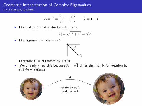
Geometric Interpretation of Complex Eigenvalues2 × 2 example, continued

A = C =

(1 −11 1

)λ = 1− i

I The matrix C = A scales by a factor of

|λ| =√

12 + 12 =√

2.

I The argument of λ is −π/4:

λ

π4

Therefore C = A rotates by +π/4.I (We already knew this because A =

√2 times the matrix for rotation by

π/4 from before.)

A

rotate by π/4

scale by√

2

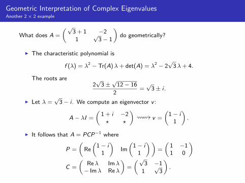
Geometric Interpretation of Complex EigenvaluesAnother 2 × 2 example

What does A =

(√3 + 1 −2

1√

3− 1

)do geometrically?

I The characteristic polynomial is

f (λ) = λ2 − Tr(A)λ+ det(A) = λ2 − 2√

3λ+ 4.

The roots are2√

3±√

12− 16

2=√

3± i .

I Let λ =√

3− i . We compute an eigenvector v :

A− λI =

(1 + i −2? ?

)v =

(1− i

1

).

I It follows that A = PCP−1 where

P =

(Re

(1− i

1

)Im

(1− i

1

))=

(1 −11 0

)C =

(Reλ Imλ− Imλ Reλ

)=

(√3 −1

1√

3

).

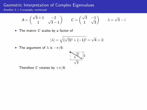
Geometric Interpretation of Complex EigenvaluesAnother 2 × 2 example, continued

A =

(√3 + 1 −2

1√

3− 1

)C =

(√3 −1

1√

3

)λ =√

3− i

I The matrix C scales by a factor of

|λ| =

√(√

3)2 + (−1)2 =√

4 = 2.

I The argument of λ is −π/6:

λ

π6 1

√3

Therefore C rotates by +π/6.

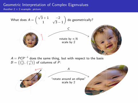
Geometric Interpretation of Complex EigenvaluesAnother 2 × 2 example: picture

What does A =

(√3 + 1 −2

1√

3− 1

)do geometrically?

C

rotate by π/6scale by 2

A = PCP−1 does the same thing, but with respect to the basisB =

{(11

),(−1

0

)}of columns of P:

A

“rotate around an ellipse”scale by 2

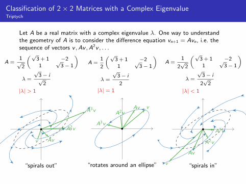
Classification of 2 × 2 Matrices with a Complex EigenvalueTriptych

Let A be a real matrix with a complex eigenvalue λ. One way to understandthe geometry of A is to consider the difference equation vn+1 = Avn, i.e. thesequence of vectors v ,Av ,A2v , . . .

A =1√

2

(√3 + 1 −21

√3− 1

)λ =

√3− i√

2

|λ| > 1

v Av

A2v

A3v

“spirals out”

A =1

2

(√3 + 1 −21

√3− 1

)λ =

√3− i

2

|λ| = 1

vAvA2v

A3v

“rotates around an ellipse”

A =1

2√

2

(√3 + 1 −21

√3− 1

)λ =

√3− i

2√

2

|λ| < 1

A3v

A2v

Av

v “spirals in”

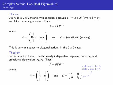
Complex Versus Two Real EigenvaluesAn analogy

TheoremLet A be a 2× 2 matrix with complex eigenvalue λ = a + bi (where b 6= 0),and let v be an eigenvector. Then

A = PCP−1

where

P =

| |Re v Im v| |

and C = (rotation) · (scaling).

This is very analogous to diagonalization. In the 2× 2 case:

TheoremLet A be a 2× 2 matrix with linearly independent eigenvectors v1, v2 andassociated eigenvalues λ1, λ2. Then

A = PDP−1

where

P =

| |v1 v2

| |

and D =

(λ1 00 λ2

).

scale x-axis by λ1

scale y -axis by λ2

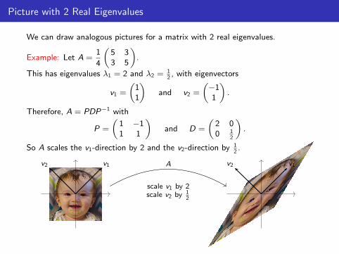
Picture with 2 Real Eigenvalues

We can draw analogous pictures for a matrix with 2 real eigenvalues.

Example: Let A =1

4

(5 33 5

).

This has eigenvalues λ1 = 2 and λ2 = 12, with eigenvectors

v1 =

(11

)and v2 =

(−11

).

Therefore, A = PDP−1 with

P =

(1 −11 1

)and D =

(2 00 1

2

).

So A scales the v1-direction by 2 and the v2-direction by 12.

v1v2 v1v2A

scale v1 by 2scale v2 by 1

2

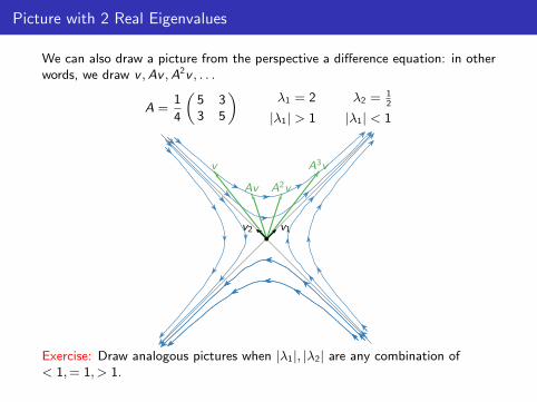
Picture with 2 Real Eigenvalues

We can also draw a picture from the perspective a difference equation: in otherwords, we draw v ,Av ,A2v , . . .

A =1

4

(5 33 5

)λ1 = 2

|λ1| > 1

λ2 = 12

|λ1| < 1

v

Av A2v

A3v

v1v2

Exercise: Draw analogous pictures when |λ1|, |λ2| are any combination of< 1,= 1, > 1.

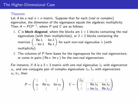
The Higher-Dimensional Case

TheoremLet A be a real n × n matrix. Suppose that for each (real or complex)eigenvalue, the dimension of the eigenspace equals the algebraic multiplicity.Then A = PCP−1, where P and C are as follows:

1. C is block diagonal, where the blocks are 1× 1 blocks containing the realeigenvalues (with their multiplicities), or 2× 2 blocks containing the

matrices

(Reλ Imλ− Imλ Reλ

)for each non-real eigenvalue λ (with

multiplicity).

2. The columns of P form bases for the eigenspaces for the real eigenvectors,or come in pairs ( Re v Im v ) for the non-real eigenvectors.

For instance, if A is a 3× 3 matrix with one real eigenvalue λ1 with eigenvectorv1, and one conjugate pair of complex eigenvalues λ2, λ2 with eigenvectorsv2, v 2, then

P =

| | |v1 Re v2 Im v2

| | |

C =

λ1 0 00 Reλ2 Imλ2

0 − Imλ2 Reλ2

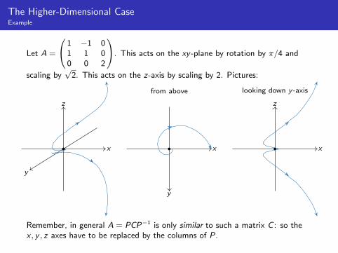
The Higher-Dimensional CaseExample

Let A =

1 −1 01 1 00 0 2

. This acts on the xy -plane by rotation by π/4 and

scaling by√

2. This acts on the z-axis by scaling by 2. Pictures:

x

y

z

x

y

from above

x

z

looking down y -axis

Remember, in general A = PCP−1 is only similar to such a matrix C : so thex , y , z axes have to be replaced by the columns of P.